 Travis Wiederstein1
 Vaishali Sharda1*
 Jonathan Aguilar2
 Trevor Hefley3
 Ignacio Antonio Ciampitti4
 Ajay Sharda1
 Kelechi Igwe1
- 1Department of Biological and Agricultural Engineering, Kansas State University, Manhattan, KS, United States
- 2Southwest Research-Extension Center, Kansas State University, Garden City, KS, United States
- 3Department of Statistics, Kansas State University, Manhattan, KS, United States
- 4Department of Agronomy, Kansas State University, Manhattan, KS, United States
Variable rate irrigation (VRI) requires accurate knowledge of crop water demands at the sub-field level. Existing VRI practices commonly use one or more variables like soil electrical conductivity, historical yields, and topographic maps to delineate variable rate zones. However, these data sets do not quantify within season variability in crop water demands. Crop coefficients are widely used to help estimate evapotranspiration (ET) at different stages of a crop’s growth cycle, and past research has shown how remotely sensed data can identify differences in crop coefficients at regional and field levels. However, the amount of spatial and temporal variation in crop coefficients at the sub-field level (i.e. within a single center pivot system) has not been widely researched. This study aims to compare sub-field ET estimates from two remote sensing platforms and quantify spatial and temporal variations in aggregated sub-field level ET. Vegetation indices and reference ET data were collected at Kansas State University’s Southwest Research Extension Center (SWREC) and two Water Technology Farms during the 2020 corn growing season. Weekly maps of the Normalized Difference Vegetation Index (NDVI) and the Soil Adjusted Vegetation Index (SAVI) from aerial imagery are combined with empirical equations from existing literature to estimate both basal and combined crop coefficients at a 1-meter resolution. These ET estimates are aggregated to a 30 m resolution and compared to the Landsat Provisional Actual ET dataset. Finally, actual ET estimates from aerial images were aggregated using k-means clustering and stationary variable speed zones to determine if there is enough variation in actual ET at the sub-field level to build variable rate irrigation schedules. An equivalence test demonstrated that the aerial imagery and Landsat data sources produce significantly different crop coefficient estimates. However, the two datasets were moderately correlated with Pearson’s product-moment correlation coefficients ranging from -0.95 to 0.86. Both the aerial imaging and Landsat datasets showed high variability in crop coefficients during the first 5-6 weeks after emergence, with these coefficients becoming more spatially uniform later in the growing season. These crop coefficients may help irrigators make more informed irrigation management decisions during the growing season. However, more research is needed to validate these remotely sensed ET estimates and integrate them into an irrigation decision support system.
Introduction
The High Plains Aquifer supports roughly one-third of all groundwater used for irrigation in the United States, making it vitally linked to the nation’s economic and food security (Dennehy et al., 2002). Despite the aquifer’s importance, poor management, overexploitation, and slow recharge has led to a decrease in the aquifer’s storage. Without proper interventions, up to 35% of the aquifer might not support irrigation by 2040 (Scanlon et al., 2012). Integrated satellite-based technologies for irrigation management decision making could lower HPA withdrawals by about 31% (Deines et al., 2019). Irrigators in the High Plains Region use several irrigation scheduling techniques such as deficit irrigation scheduling, where soil moisture content is allowed to deplete to a crucial threshold before irrigation is triggered (Rudnick et al., 2019; Ajaz et al., 2020). This method is especially effective during non-critical growth stages. Under both deficit and non-deficit irrigation scheduling, producers typically apply a uniform amount of water to an entire field. However, actual crop demands can vary through space and time (spatiotemporally) based on plant density, growth stage, plant health, topography, soil properties, crop genetics, and the presence of pests or diseases, among many other factors (Evans et al., 2013). To meet these variable demands, researchers and agricultural technology companies have developed speed control systems and flow rate control systems. These Variable Rate Irrigation (VRI) technologies can be retrofitted to existing center pivots and allow producers to apply different amounts of water to different parts of a field.
Both deficit irrigation and VRI require knowledge of crop water demands at high spatial and temporal scales. Past researchers and agricultural technology companies have used physical soil properties, historical yield data, and in situ sensors to estimate crop water demand at sub-field scales (Garg et al., 2016; Sui, 2017). However, physical soil properties and historical data only provide an indirect way to predict crop water demands, and they do not typically represent in-season changes to water demands. While sensor networks, most commonly soil moisture or crop canopy sensors, provide in-season estimates of crop water demands, they can be expensive, intrusive to normal agricultural operations, and they cannot take measurements across the entire field. In contrast, remote sensing platforms can provide in-season information about crop water demands without the need for in-field sensors. Specifically, the integration of multispectral and thermal sensing into irrigation management systems has assisted in monitoring live plant and soil water stress (Blonquist Jr. et al., 2005; O’Shaughnessy & Evett, 2008; Evett et al., 2009; Mahan et al., 2010; O’Shaughnessy and Evett, 2010; Casanova et al., 2012) and may be useful for informing VRI schedules (Maguire and Neale, 2022). Existing research has converted data from these sensors to water stress indices, which are compared to critical values (Espinoza et al., 2017). Once the measured index reaches a critical threshold, irrigation is triggered. Multiple decision support systems are available to integrate these indices into the VRI scheduling process (Liakos et al., 2015; Shi et al., 2019; Andrade et al., 2020; Evett et al., 2020; Stone et al., 2020).
While the introduction of these new indices has advanced the practicality of VRI, typical VRI decision support systems are still incapable of providing support based on both high spatial and temporal resolution estimates of crop water demands (Tolomio and Casa, 2020). Additionally, decision support systems based on water stress indices typically require knowledge of local, experimentally determined critical stress thresholds. However, data for traditional evapotranspiration-based irrigation scheduling is often readily available from national-, state-, or university-funded sensor networks, like the Kansas Mesonet (http://mesonet.k-state.edu/weather/historical). The Kansas Mesonet is a network of over 60 weather stations that estimates reference evapotranspiration (ET) values across the state of Kansas. Multiple methods exist to convert these reference ET values to actual crop ET, including the use of single and dual crop coefficients. The single crop coefficient method uses a single coefficient (Kc) to adjust reference ET values to actual ET based on crop characteristics and averaged effects of soil evaporation (Doorenbos and Pruitt, 1977). In contrast, the dual crop coefficient method splits this Kc value into two components—one for plant transpiration (Kcb), and one for soil evaporation (Ke) (Allen et al., 2005a). Both Kc and Kcb vary based on crop and plant growth stage. However, growth stages are typically only divided between early, mid, and late season, and do not reflect daily changes in crop water demands. Ke is calculated as a function of the amount of water available in the soil for evaporation, and the fraction of the soil’s surface that is exposed and wetted. Both single and dual crop coefficients are useful for irrigation scheduling, but neither have been widely used for variable rate irrigation due to a lack of knowledge of the crop growth stages and soil water availability at the sub-field level.
New sources of remote sensing information may be useful for identifying high spatial and temporal differences in crop ET coefficients. Remote sensing, especially satellite imagery, is often used to study changes in vegetation properties, including crop coefficients, at national, regional, and field scales. However, satellite images are not always available at the right time, or the right spatial resolution to be useful for agricultural management. In contrast, drones have been used as a remote sensing platform in agriculture for plant emergence monitoring, weed detection, crop damage or illness mapping, and crop water stress mapping to detect equipment malfunctions (van der Merwe et al., 2020). However, collecting and processing drone data can be very time-consuming and labor-intensive. Multispectral cameras mounted to small commercial aircraft can collect similar data at a 1-meter spatial resolution, and a temporal resolution of up to a week, which may be ideal for making more informed in-season management decisions. However, data from these three sources have not been used to determine if there are high enough spatial and temporal differences in crop coefficients to inform VRI schedules.
This study was undertaken to conduct a comparison of remotely sensed crop coefficients and actual ET estimates from two different platforms: Landsat 8’s Provisional Actual Evapotranspiration data set and aircraft-based multispectral imagery. While each platform uses similar data (i.e., multispectral images) to estimate spatial patterns of actual ET and crop coefficients, each platform has its own processes for atmospheric correction and conversion of reflectance measurements to ET. Each platform also measures a different range of the electromagnetic spectrum, and each platform has its own limitations to its usefulness in informing in-season management decisions based on its spatial and temporal resolution. The purpose of this study is to identify if these platforms can identify high enough spatial and/or temporal differences in crop ET to develop dynamic variable rate irrigation schedules.
Methods
Site descriptions
All data were collected on irrigated corn fields during the 2020 growing season. The two quarter circle plots (Figures 1A, B) were located on producer-owned fields and are part of Kansas Water Office’s Water Technology Farm program. Field A is located approximately 17 km Northeast of Leoti, Kansas, and Field B is located 17.5 km Northwest of Garden City, Kansas. The East half of the experimental center pivot (Figure 1C) is on a quarter section of land that is owned and operated by Kansas State University’s Southwest Research and Extension Center (SWREC), located 4.8 km Northeast of Garden City, Kansas. This region is characterized by a humid subtropical climate, an average of 35-50 cm of annual precipitation, and Richfield series silt-loam soils. During this study, the research plot was primarily used by SWREC to test different irrigation application technologies, like different nozzle types and application rates. Field A and Field B are characterized by similar soils and climate as those at the SWREC research plot. Crop growth stages were monitored during weekly visits to each location.
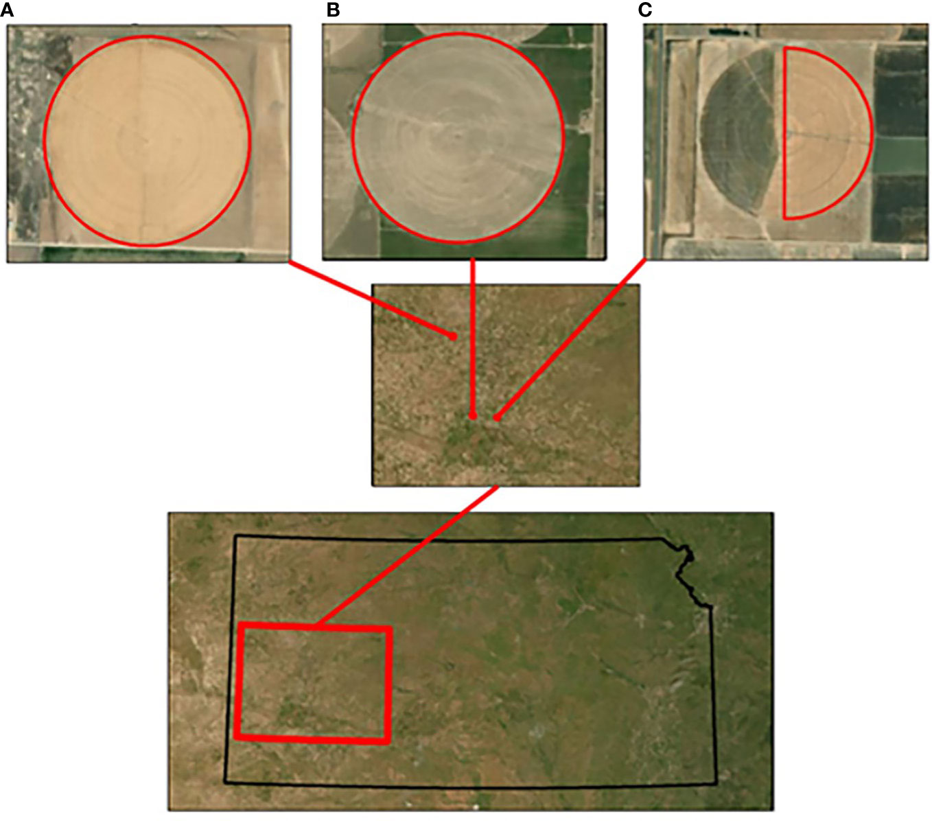
Figure 1 Experimental site locations. (A) Field A (B) Field B and (C) KSU SWREC.
Data sources and descriptions
Kansas Mesonet stations located near Field B and the SWREC plot measured air temperature, relative humidity, solar radiation, wind speed, wind direction, barometric pressure, and soil temperature throughout the growing season. The Kansas Mesonet uses these measurements to calculate daily reference ET using the ASCE standardized reference evapotranspiration equation (Allen et al., 2005b). Reference ET values from the Leoti Kansas Mesonet Station located 55 km North of Field A were used in lieu of an on-site weather station for Field A. More information regarding the Kansas Mesonet weather stations, including a history of their development, is provided by Patrignani et al. (2020). An agricultural technology company collected thermal and multispectral images of each location at one-week intervals. The spatial resolution of each aerial image varied from 0.8 meter to 1.1 meters by location and collection date based on the elevation of the aircraft-mounted sensors during the data collection flight. Each image was orthorectified and atmospherically corrected by the agricultural technology company. These images were also reprojected and resampled to the lowest available spatial resolution using tools available in the raster R package (Hijmans, 2020). Reprojecting and resampling these images to the same extent and resolution allows for a pixel-by-pixel comparison of the reflectance values from each measurement date. 30-meter fractional ET images from the Landsat satellite series were downloaded from the EarthExplorer database and are functionally equivalent to crop coefficient maps. This data is provided courtesy of the United States Geological Survey, and was developed by (Senay, 2018). The images are available in 298-square-kilometer scenes and can be filtered to only include images with limited cloud coverage. In contrast to the aerial images, which are collected during ideal flight conditions, the Landsat satellites have a fixed return period of about 16 days, meaning images of the fields are not available if the satellite passes over each location on a cloudy day. For this study, the Landsat images were filtered to only include those with 10% cloud coverage or less. Finally, the spectral resolutions of the aerial imaging platform and Landsat platform vary slightly, but they both measure wavelengths in the near infrared (NIR) and visible red regions of the electromagnetic spectrum. Therefore, no spectral adjustments were made to either dataset.
Conversion of vegetation indices to crop coefficients
Pôças et al. (2020) provides a review of techniques and best practices for converting multispectral imagery to single and basal crop coefficients. Their review includes regression equations from existing literature that estimate crop coefficients from the Normalized Difference Vegetation Index (NDVI) and the Soil Adjusted Vegetation Index (SAVI). Six of these equations were used to calculate irrigated maize crop coefficients from the aerial and Landsat images described above. These equations are presented in Table 1 along with information regarding their development. It is worth noting that these equations were developed using a variety of multispectral sensors, and not all the publications included measurements of uncertainty or error compared to in situ measurements. Out of the equations listed, Kamble et al. (2013) provided the most detailed comparison to in situ data. Their research presented combined crop coefficients with root-mean-squared-errors between 0.16 and 0.19 relative to values calculated from the AmeriFlux sensor network in the High Plains region.
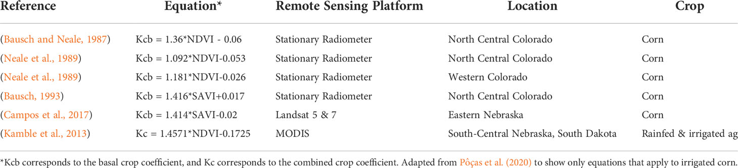
Table 1 Linear models correlating corn evapotranspiration coefficients to vegetation indices derived from multispectral reflectance.
Comparison of aerial imagery and landsat data
The aerial multispectral images were converted to NDVI and SAVI using equations 1 and 2 below, which were originally developed by Rouse et al. (1974) and Huete (1988), respectively. After calculating the NDVI and SAVI values for every pixel in the aerial dataset using these equations below, the linear equations from Table 1 were used to create maps of crop coefficients. These crop coefficient maps were multiplied by the daily Kansas Mesonet reference ET to create maps of actual crop ET for each data collection date. The ET values calculated using the basal crop coefficient equations mentioned Pôças et al. (2020), are primarily driven by crop transpiration. In contrast, the ET value calculated using the combined crop coefficient equation mentioned in Pôças et al. (2020) is driven by both transpiration and surface evaporation.
where:
NDVI = Normalized Difference Vegetation Index
NIR = Percent reflectance of light in the near-infrared region of the electromagnetic spectrum
R = Percent reflectance of light in the red region of the electromagnetic spectrum
where:
SAVI = Soil Adjusted Vegetation Index
L = Soil brightness correction factor, assumed to be 0.5
Given the differences in spatial and temporal resolutions between these datasets, additional processing was completed to compare the ET maps. To directly compare the aerial and Landsat ET estimates, ET maps from both sources were reprojected to WGS 84 UTM Zone 14N using ArcGIS 10.4.1 (ESRI, 2011) to minimize distortion and clipped to the extent of the irrigated area at each site. To account for the difference in temporal resolution, the aerial imaging crop coefficient maps were linearly interpolated to a daily time step. This interpolation allows for an approximate same-day comparison between the Landsat and aerial ET estimates. Additionally, the aerial maps were chosen over the Landsat maps for interpolation because of their finer temporal resolution. This finer temporal resolution produces less uncertainty during interpolation relative to interpolated predictions of the lower temporal resolution Landsat data. Finally, the aerial images were aggregated to a 30-meter resolution by taking the mean crop coefficients from all 0.8-meter pixels that overlapped a given Landsat pixel.
Delineation of ET zones and zone aggregation
In addition to accurately predicting actual ET, remote sensing platforms must demonstrate sufficient variation in sub-field level ET to be useful for VRI scheduling. However, what justifies “sufficient” variation between management zones is highly dependent on the level of control an irrigator has over their pivot system. Two types of control are most common: center pivot speed control, that creates pie slice shaped VRI zones, and span control that creates concentric gridded VRI zones (Kranz et al., 2012). To mimic VRI schedules for both control techniques, the aerial ET maps were spatially aggregated into VRI zones using two different techniques. First, mock pivot speed control zones were created by dividing the center pivots into 2-degree-wide slices, resulting in 90 different VRI zones for the experimental half pivot, and 180 VRI zones for Fields A and B.
Second, the kmeans function from the stats package in R (R Core Team, 2022) was used to build maps of crop water demands useful for systems with zone control, where irrigators can change flow rates to individual spans, or clusters of a few nozzles. The ideal number of clusters for k-means clustering is commonly calculated using the elbow method, which graphs the within-cluster sum of squares for k number of clusters, where k ranges from 1 to some large number, and identifies the point where additional clusters produce minimal reductions in the within cluster sum of squares (WSS). K-means clustering was chosen to maximize the difference in irrigation depths between each zone and mimic the type of zones that would be created from a variable flow control system. This unsupervised classification technique assigns each image pixel individually to one of k groups. This is done in iterations, and attempts to minimize within cluster variance calculated as WSS:
where:
WSS = within cluster (or zone) sum of squares
k = number of clusters
n = number of observations in the jth cluster
xi(j) = ith observation in the jth cluster
cj = jth cluster centroid
The elbow method was used to determine the appropriate number of clusters for k-means clustering. This method plots the total WSS for 1 to k clusters. The “elbow” in this line plot corresponds to the location where diminishing reductions in the total WSS occur with increasing k. Given that the goal of this research is to identify a potential alternative to multi-variate zone delineation techniques, no covariates were used in the clustering process.
Crop coefficient maps using the linear regression equation from Kamble et al. (2013) were used for zone creation since this equation represents a combined soil and crop evapotranspiration coefficient, rather than just a basal crop coefficient. Each zone’s irrigation depth was calculated by summing the daily ET maps at the end of every 7-day period after the crop emergence date. The pie zones were aggregated using the mean of all cells in each zone.
While VRI using these crop coefficient maps does not change the total volume of water used, they could improve how water is allocated within a field if zones are properly delineated. Ideally, these maps would improve water use efficiency, which is defined as the amount of biomass production per unit of water (Briggs and Shantz, 1913). Here, two types of variable rate zone delineations are evaluated based on their ability to account for spatial variability in crop water demands, which is quantified using the mean distance from the centroid. Ideally, variability within each zone (meaning the mean distance from the centroid) will be minimized, and the variability between zones will be maximized. This indicates that the aggregated ET values are an accurate representation of the crop water demands within each zone, and irrigation is properly distributed across the entire field. The mean distance from the centroid is calculated as:
Where:
J = mean distance from the centroid
k = number of clusters (or zones)
n = number of observations in the jth cluster
xi(j) = ith observation in the jth cluster
cj = jth cluster centroid
Results and discussion
Comparison of aerial imagery and landsat datasets
Boxplots of mapped crop coefficients for Fields A and B are shown by collection date in Figures 2, 3. The median crop coefficients from both datasets follow a seasonal pattern similar to traditional crop coefficient curves, except for the July 6th Landsat estimates. These boxplots capture both the spatial and temporal variability in the crop coefficient estimates throughout the growing season. Generally, the interquartile range from the aerial imagery-based estimates appears to decrease for both locations as the season progresses. In comparison, the Landsat-based crop coefficient estimates show consistently wider interquartile ranges throughout the entire growing season. Additionally, the SAVI-based crop coefficients show greater sub-field variability later in the season when the crop canopy is heavily developed.
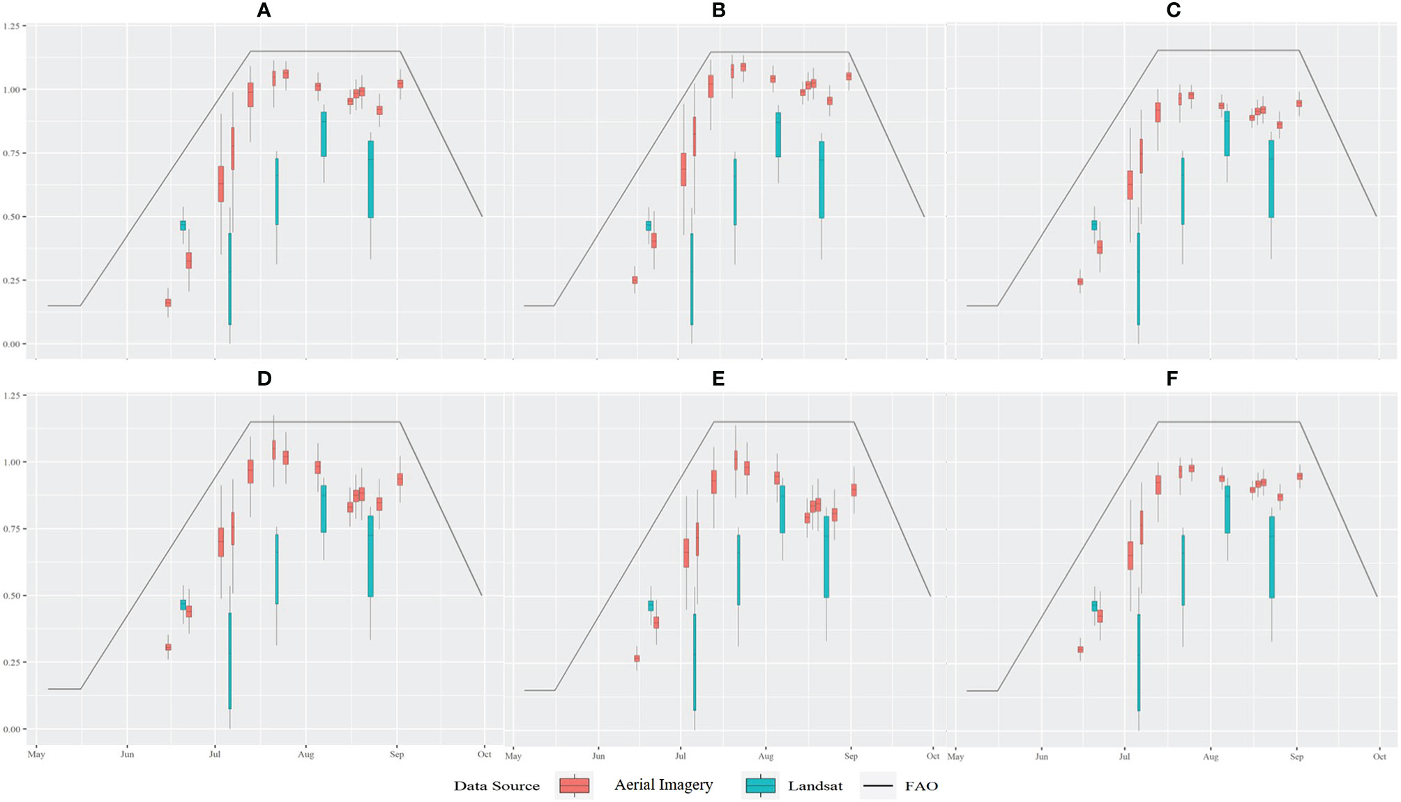
Figure 2 Boxplots of crop coefficients at Field A from Landsat and Aerial Imaging. Crop coefficients were estimated from equations developed by (A) Kamble et al. (2013), (B) Bausch and Neale (1987), (C) Bausch and Neale (1987), (D) Bausch (1993), (E) Campos et al. (2017), and (F) Neale et al. (1989).
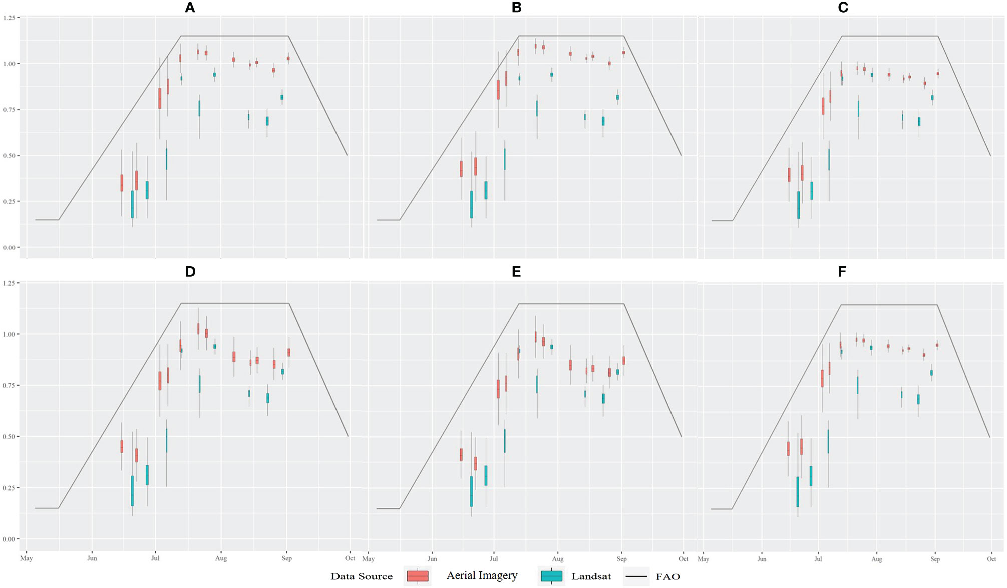
Figure 3 Boxplots of crop coefficients at Field B from Landsat and Aerial Imaging. Crop coefficients were estimated from equations developed by (A) Kamble et al. (2013), (B) Bausch and Neale (1987), (C) Bausch and Neale (1987), (D) Bausch (1993), (E) Campos et al. (2017), and (F) Neale et al. (1989).
All the linear regression equations and data combinations produced higher ET estimates than the Landsat data. Additionally, the Landsat estimates most closely approximate the aerial imagery values calculated using the regression equation from Kamble et al. (2013). This is likely because the Kamble et al. equation predicts the combined crop coefficient, which accounts for both soil and plant transpiration, compared to the other equations which only predict the basal crop coefficient. Given that the pixels in the aerial imagery covered both vegetated and bare soil surfaces, the combined crop coefficient model from Kamble et al. (2013) is a more accurate representation of real-world conditions compared to the basal crop coefficient models. The NDVI-based linear models predicted less variability in crop coefficients than the SAVI-based linear models and satellite-based crop coefficients. This is a phenomenon noted by Neale et al. (1990), who found that NDVI-crop coefficient relationships are not accurate past full canopy cover development. This is because NDVI becomes insensitive to differences in canopy coverage past a leaf area index of 2-3 (Myneni et al., 1997).
To better understand what causes these differences, the sum of the differences between all Landsat collections dates were mapped (Figures 4–6). The sum of differences was preferred over the sum of squares of the differences to identify parts of each field that were over or underestimated. Spatially, the greatest differences between these two data sets occurred around the field boundaries. This is likely due to the difference in spatial resolutions of the datasets. The higher resolution aerial images provide a more accurate delineation of the boundary between crops and the surrounding unplanted area. This concept of “mixed pixels” is common to studies using remote sensing data and is further discussed in relation to agricultural management practices by (Ines and Honda, 2005). The unplanted areas around the center pivot boundaries have lower crop coefficients values since they are not heavily vegetated. Therefore, the lower resolution Landsat images may be under-predicting the crop coefficients values near the field boundaries, given that a single Landsat pixel includes both planted and unplanted land.
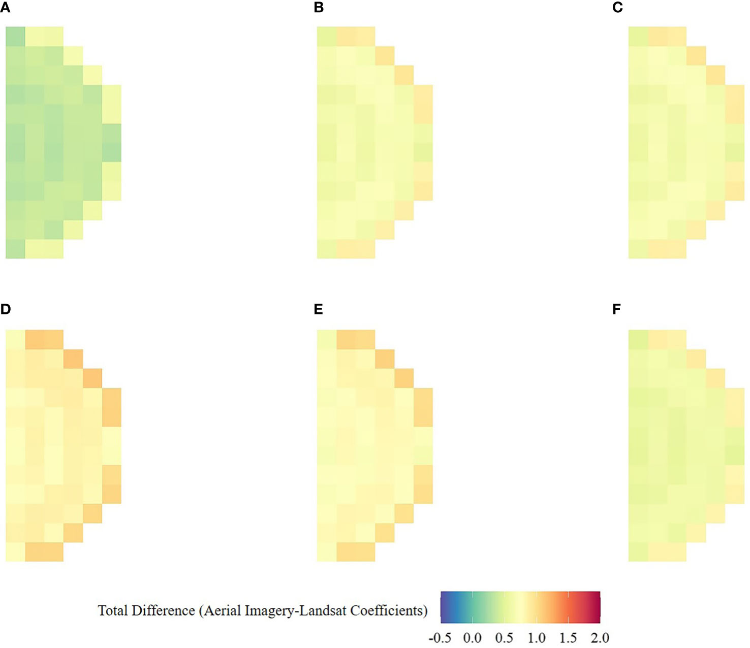
Figure 4 Total seasonal differences between the Aerial Imaging crop coefficients and the Landsat Fractional ET Data at Field (A) Aerial Imaging crop coefficients were estimated from equations developed by (A) Kamble et al. (2013), (B) Bausch and Neale (1987), (C) Bausch and Neale (1987), (D) Bausch (1993), (E) Campos et al. (2017) and (F) Neale et al. (1989).
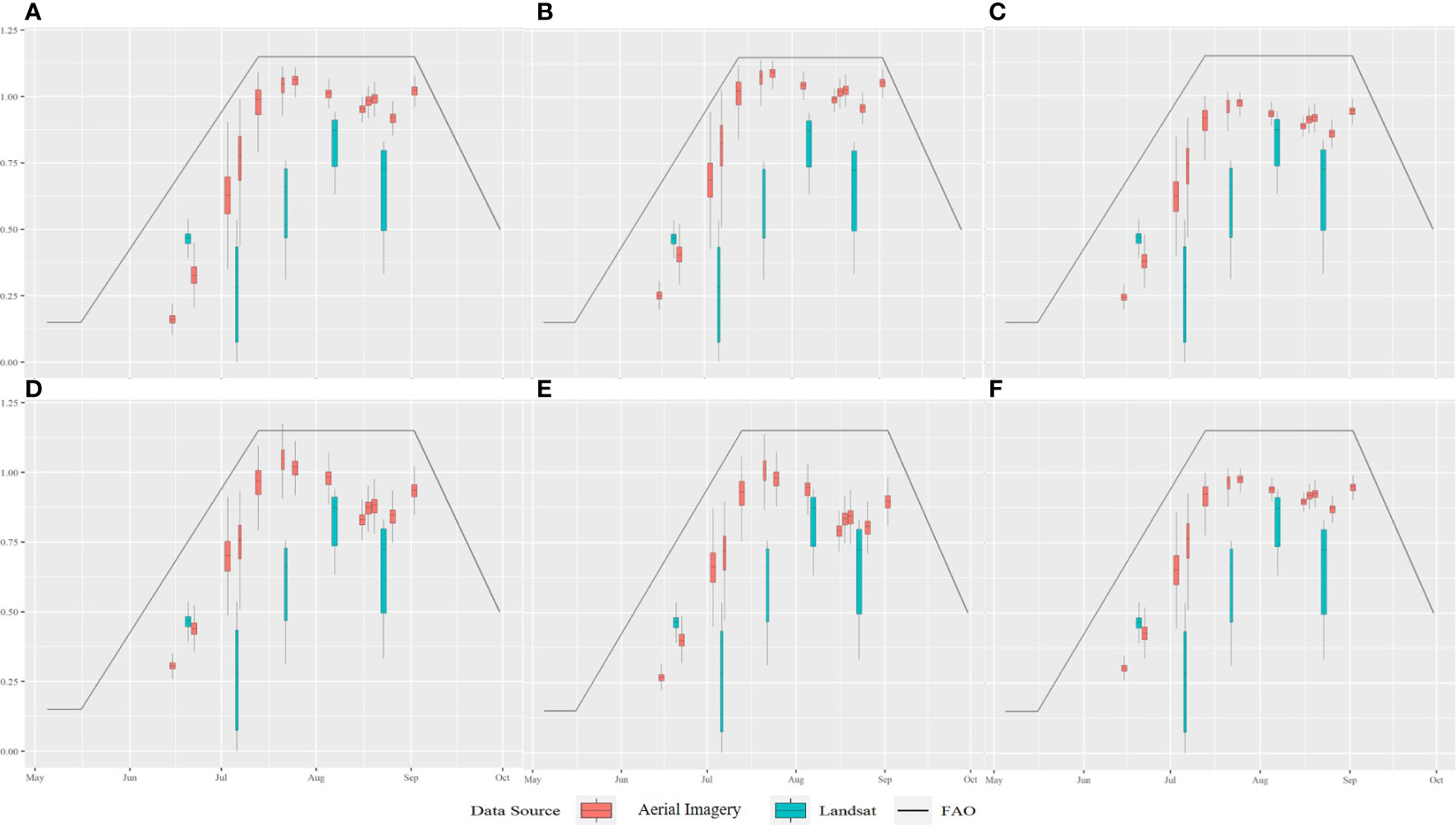
Figure 5 Total seasonal differences between the Aerial Imaging crop coefficients and the Landsat Fractional ET Data at Field (B) Aerial Imaging crop coefficients were estimated from equations developed by (A) Kamble et al. (2013), (B) Bausch and Neale (1987), (C) Bausch and Neale (1987), (D) Bausch (1993), (E) Campos et al. (2017), and (F) Neale et al. (1989).
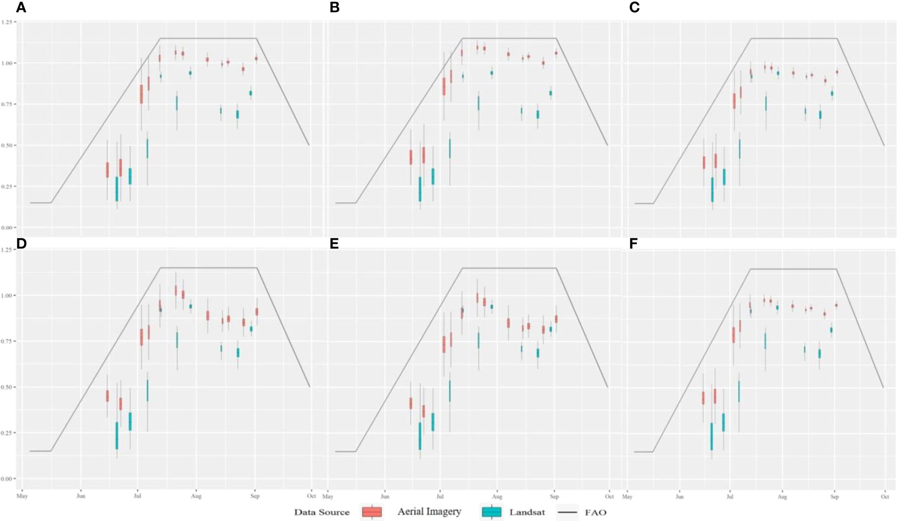
Figure 6 Total seasonal differences between the Aerial Imaging crop coefficients and the Landsat Fractional ET Data at the SWREC. Aerial Imaging crop coefficients were estimated from equations developed by (A) Kamble et al. (2013), (B) Bausch and Neale (1987), (C) Bausch and Neale (1987), (D) Bausch (1993), (E) Campos et al. (2017), and (F) Neale et al. (1989).
While the maps above identify spatial differences between the Landsat and aerial imagery crop coefficients estimates, they do not demonstrate the impact of differences in these coefficients on the whole field’s evapotranspiration. To better understand the impact of these differences in values on the total ET volume, the original ~0.8-meter resolution Kc maps were multiplied by the daily reference ET and raster cell area, then summed. The same process was repeated for the 30-meter Kc rasters from the Landsat images to produce a whole-field ET estimate. These whole-field ET estimates are given in Table 2.
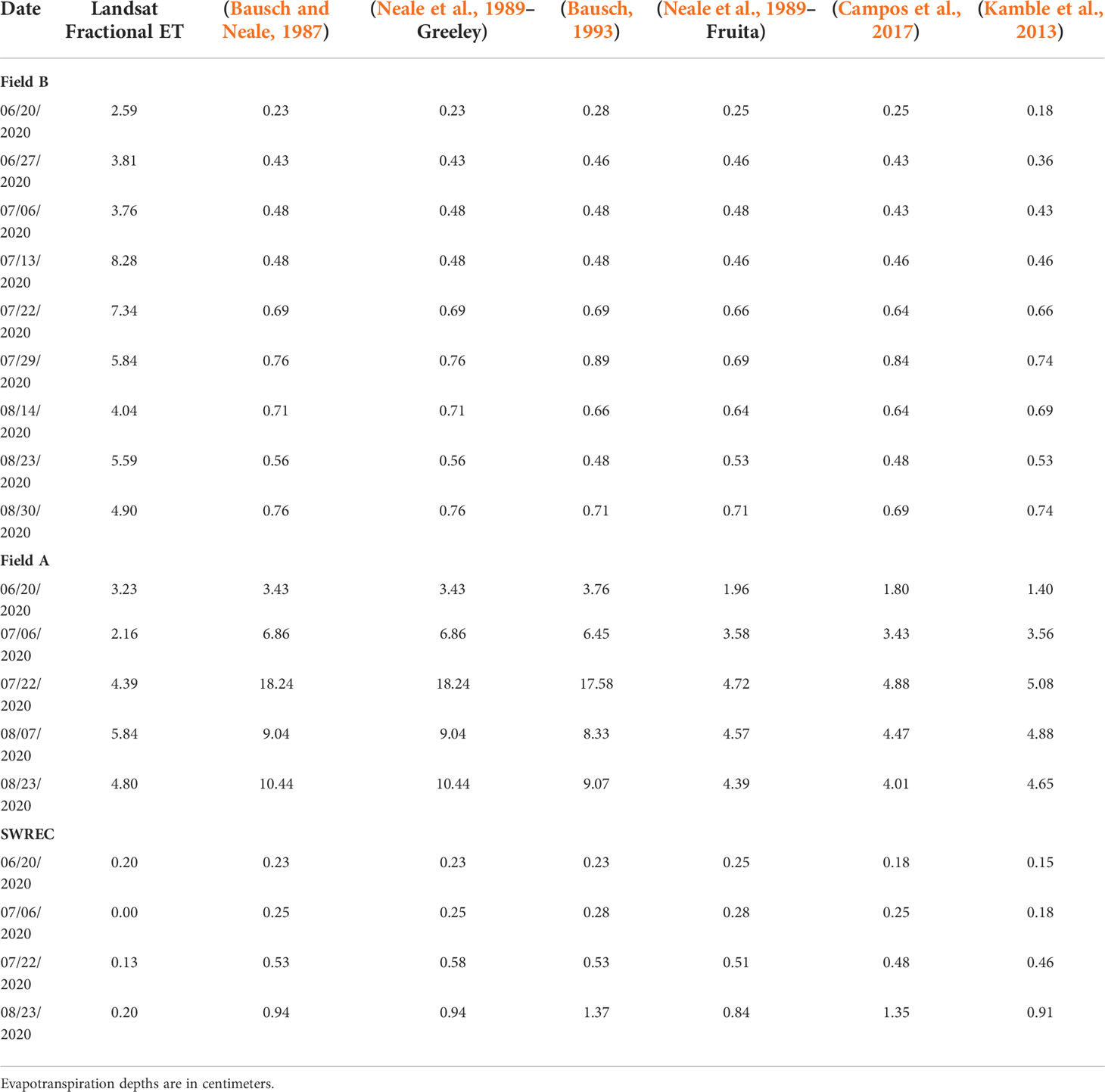
Table 2 Whole field actual evapotranspiration estimates calculated based on seven different crop coefficient maps.
Lastly, the correlation between the aggregated aerial imagery and Landsat Kc estimates was assessed using Pearson’s product-moment correlation. Arguably, an equivalence test would be preferred to a correlation test, given the data sources are attempting to measure the same parameter. However, the Landsat and aerial imagery Kc estimates are calculated using very different methods, and the boxplots (Figures 2, 3) show little direct equivalence between the data sources. Additionally, a Two One-Sided equivalence Test (TOST) was non-significant at an alpha of 0.05, indicating that the two data sources are statistically different. Instead, Pearson’s product-moment correlation is calculated to determine if there is a correlation between the Kc values from each source. Pearson’s coefficient has been commonly used to compare remote sensing data with in-situ and environmental variables such as evapotranspiration (Szewczak et al., 2020), above ground biomass and canopy height (Li et al., 2016), and land surface temperatures (Mudede et al., 2020). A positive Pearson coefficient close to one indicates a strong, positive correlation between variables, and values near zero indicate there is no correlation between variables.
Comparing the two datasets on a paired pixel-by-pixel basis demonstrated poor agreement between the Landsat and aerial imagery crop coefficient estimates, with a TOST concluding that the datasets are statistically different at an alpha of 0.05. However, a correlation test using Pearson’s rho demonstrated that the interpolated and aggregated crop coefficient estimates from the aerial images were moderately, and positively correlated to the Landsat Fractional ET estimates at the two producer fields (ρ = 0.86 at Field B, 0.63 at Field A) and negatively correlated at the East half SWREC center pivot (ρ = -0.95). The positive rho values close to 1 from Fields A and B indicate that the crop coefficients estimate from the two data sources were positively correlated, meaning as the estimated crop coefficients from one data source increases, so does the estimated crop coefficients from the other. The strong negative rho value at the SWREC indicates that the crop coefficient estimates from the two data sources were negatively correlated. However, the SWREC field was much smaller, meaning there were fewer data points for a pixel-by-pixel comparison. This also means that the confidence intervals of the rho estimate at the SWREC plot had a wider confidence interval. Additionally, the SWREC center pivot uses dragon lines, which drastically decreases evaporation rates from soil and crop canopies. Although evaporation accounts for most of the uncertainty in actual ET calculations, the results from the SWREC plot should be interpreted with these differences in management practices and size in mind.
Evaluation of ET Zone aggregation
The variable speed control zone delineation resulted in 180 individual management zones at Fields A and B, and 90 management zones at the SWREC half-pivot. An example of these zones is shown in Figure 7. The mean, middle 90%, and total range of weekly ET of these zones is shown for each location in Figure 8. At Field A, the mean zone ET ranged from 0.79 to 3.18 cm, the middle 90% ranged from 0.74 - 0.86 cm to 3.10 – 3.23 cm, and the range varied from 0.69 - 0.97 cm to 1.98 – 3.23 cm between the first and last weeks of the study, respectively. At Field B, the mean zone ET ranged from 1.42to 4.32 cm, the middle 90% ranged from 1.42 – 1.91 cm to 4.30 – 4.37 cm, and the total range varied from 1.24 – 1.91 cm to 4.01– 4.39 cm between the first and last weeks of the studies, respectively. Finally, at the SWREC half-pivot, the mean ET values ranged from 2.08 to 6.60 cm, the middle 90% ranged from 2.06 – 2.13 cm to 6.40 – 6.766 cm, and the total range varied from 2.03 – 2.59 cm to 6.27 – 6.78 cm between the first and last weeks of the studies, respectively.
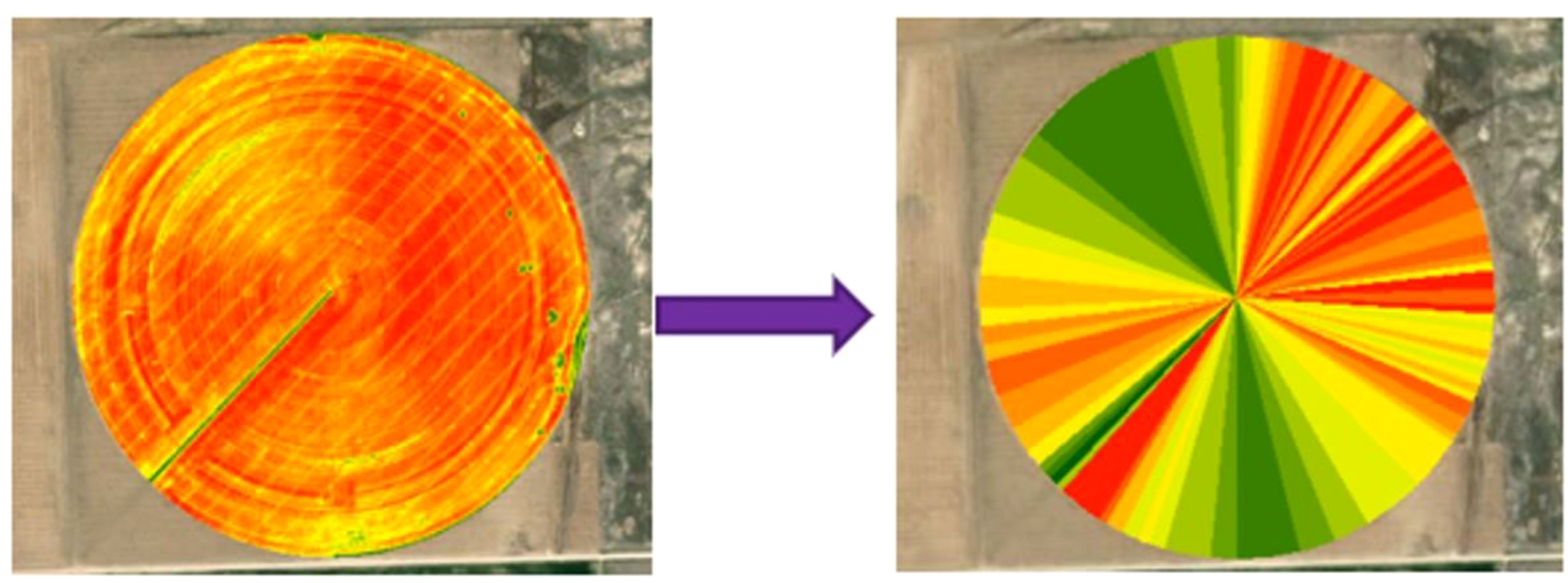
Figure 7 Weekly ET maps (left) are aggregated into variable speed control zones (right) using the mean of all pixels within each zone.
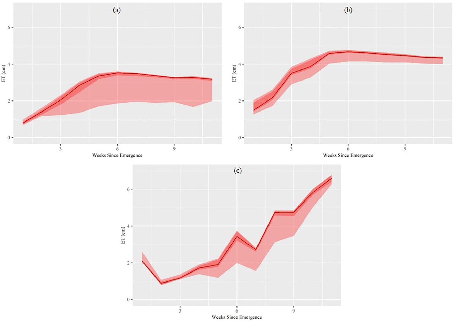
Figure 8 Mean, middle 90th percentile (dark red), and range (light red) of weekly evapotranspiration for all variable speed zones in (A) Field A, (B) Field B and (C) the SWREC Pivot.
While both data sources demonstrated variability in ET at the sub-field level, the aerial imagery’s variability decreased significantly late in the growing season and total ET did not significantly decrease with crop senescence. This is likely due to NDVI and SAVI saturation, which commonly occurs when crop canopies are fully developed. In contrast, fractional ET estimates from the Landsat Data show higher in-field variability and more significant decreases in ET late in the growing season.
Both Field A and B reached a peak weekly ET volume at around six weeks after emergence. In contrast, the SWREC East Pivot ET continued to increase throughout the data collection period due to a section of malfunctioning nozzles, which stunted a portion of the field’s growth until late in the season. The weekly ET between the middle 90th percentile of the variable speed zones (or the middle 162 zones), only differed by 0.25-0.51 cm (10-20%) for the first five weeks after emergence, then decreased to less than 0.25 cm (<10%) for the remainder of the data collection period at all locations. However, the total range of all zones’ ET values ranged from about 1.27 cm at Field B, to about 1.91 cm at Field A and the SWREC East Pivot. Overall, this demonstrates that there is a clear difference in total sub-field ET. However, sub-field ET tended to become more uniform in this study as the season progressed. Therefore, early season ET maps may help irrigators allocate resources under water-limited conditions to relieve prolonged early-season water stress, which negatively impacts final yields. However, the sub-field variability in ET decreased by tasseling and ear formation, which are considered the most critical growth stages.
Results of the k-means clustering elbow test for Field B are shown in Figure 9, which shows that four k-means clusters are sufficient for every week during the data collection period at Field B, given that the reduction in WSS is negligible with the addition of more than four clusters. The same graphs for the other two locations yielded similar results, with four clusters being sufficient for k-means clustering every week. The largest WSS occurred between two and four weeks after emergence for both the fields. In contrast, the largest WSS at the SWREC field occurred between seven and nine weeks after emergence. The WSS at the SWREC peaked later in the season due to the malfunctioning section of nozzles, which stunted the growth of a large section of plants in the middle of the pivot and increased the sub-field crop coefficients variability.
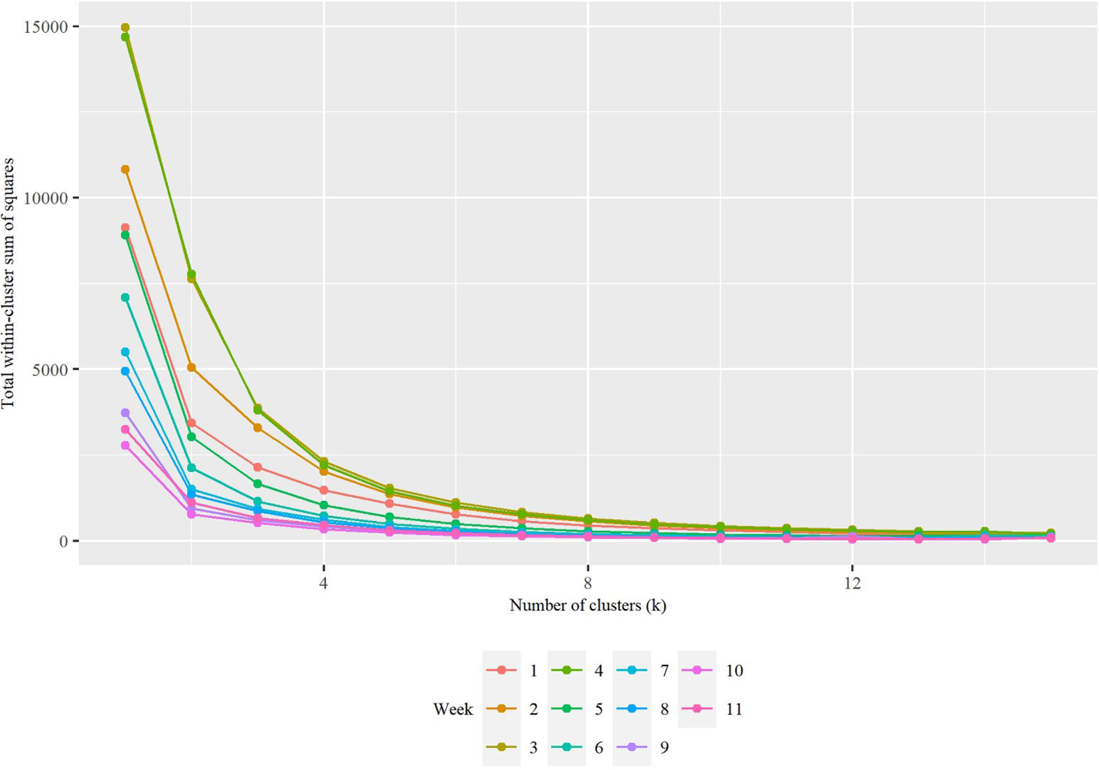
Figure 9 K-means clustering Elbow test results for Field B by week.
The centroid, or mean, value of all weekly ET pixels in each cluster was used to determine the weekly crop water demand in each zone. The weekly crop demand for each zone is shown in Table 3 and an example of a k-means clustering map is shown in Figure 10. Note that unlike the pivot speed control zones, the size and shape of each k-means cluster changes every week because the ET maps themselves are used for the VRI zone delineation. As expected, the area with the largest weekly ET tended to grow as the season progressed, which corresponds to increased crop water demands with crop maturity. By six weeks after emergence at both the fields, the k-means zone with the highest weekly ET covered approximately 70% of the entire field. Lastly, the average mean distance from the centroid for each aggregation method at each location is shown in Figure 11 for comparison.
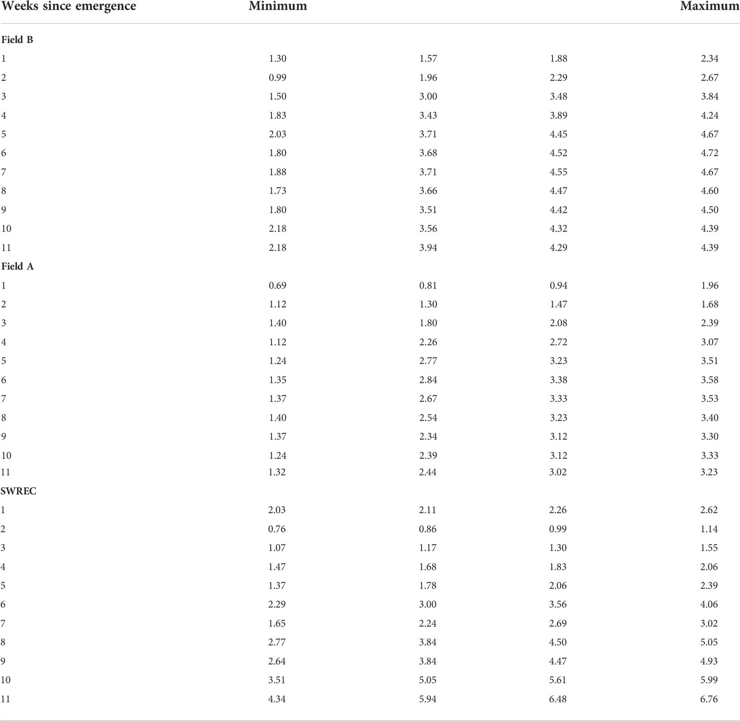
Table 3 Evapotranspiration depth (centimeters) for every k-means clustering zone, sorted by minimum depth to maximum depth.
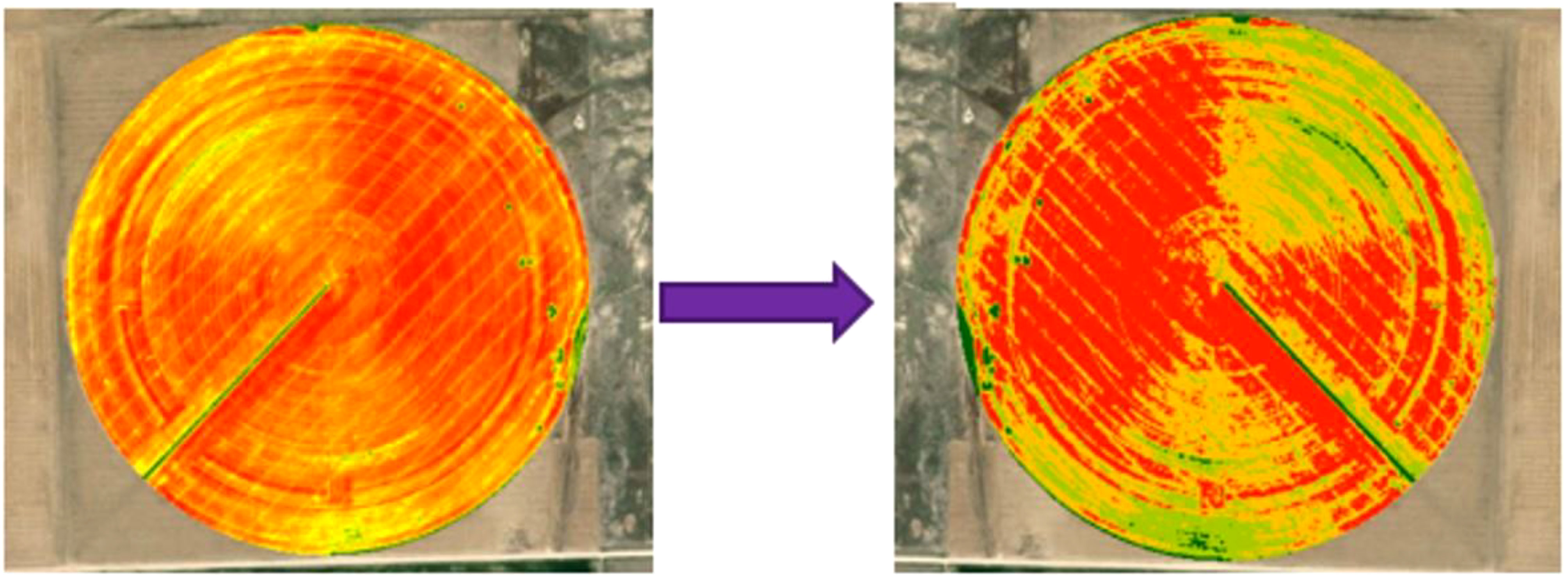
Figure 10 Weekly ET maps (left) are aggregated using k-means clustering to mimic variable flow control zones (right).
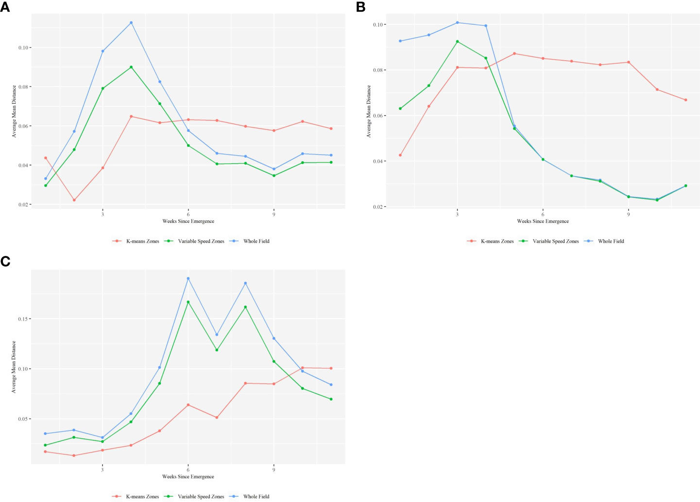
Figure 11 Time series of average mean distance from the zone’s aggregated ET value by aggregation method at (A) Field A, (B) Field B, and (C) the SWREC Pivot.
The range of mean distances from the centroid varied by date and aggregation type and was higher in the variable speed zones than in the k-means clusters. Even though the average mean distance from the centroid in the variable speed zones was less than that of the k-means clusters, there was higher variability in the mean distances in the variable speed zones. This means that the variable speed zones produced inconsistent levels of within-zone variability, while the k-means clustering produced zones with similar levels of within-zone variability. This indicates that the mean ET in some of the variable speed zones did not accurately represent the water demand in those zones. This is due to the static nature of the variable speed zones. Some of the variable seed zones contain both healthy and unhealthy or unplanted areas. Evapotranspiration increases in healthy planted areas as the season progresses, while the evapotranspiration in unplanted or damaged areas remains low. Therefore, k-means clustering is preferred over variable speed zones in fields with known regions of unplanted areas or unhealthy plants, unless these unplanted or unhealthy areas are removed from the dataset before zone delineation.
Limitations and future work
A major limitation to the comparison of remote sensing platforms used in this study was a lack of same-day data collection between the datasets. To account for this, the crop coefficients calculated from the aerial images were linearly interpolated between collection dates and aggregated to a 30-meter resolution to match the Landsat data. These methods, in combination with the Vegetation Index (VI)-Kc models introduced a significant amount of uncertainty to the actual ET estimates. Future remote sensing comparison studies should aim to eliminate, or at minimum, quantify this uncertainty by comparing data collected from different platforms on the same day. Additionally, the SSEBop model used to create the Landsat Provisional ET Dataset was developed across the contiguous United States and is commonly used for regional studies. The use of this data at the sub-field level adds an additional source of uncertainty.
In addition to the challenges of accurately quantifying late season ET previously mentioned, there are some practical limitations to using either dataset for variable rate irrigation scheduling. The most significant limitation for both datasets is a lack of validation from in situ measurements. The Landsat images have been validated using data at regional scales, but they have not been used for sub-field level management decisions (Singh et al., 2014; Senay et al., 2016; Senay et al., 2017). The second major limitation is the image processing time, which ranges from about 1-2 days for the aerial imagery, to about a week for the Landsat images. It is imperative for irrigators to make well-informed decisions at the right time to avoid unnecessary crop stress that could negatively impact yields. Third, aerial imagery providers offer a wide variety of products for both water and nutrient stress monitoring, as well as customized insight into their data. However, for some, these services may not be cost effective at the frequency needed for irrigation scheduling. In contrast, the Landsat Provisional ET Dataset is available for free, but the raw data does not have the same level of support or insight that aerial imagery provides. Additionally, the Landsat satellites have a fixed revisit period, meaning they may not always collect data under ideal environmental conditions (i.e., rainy or cloudy days).
This work presents several opportunities for future research to improve on the comparison of crop evapotranspiration monitoring using remote sensing platforms. First, the introduction of uncertainty could be reduced by carefully planning data collection to occur on the same date, and as close to the same time, for all data sources. This would eliminate the need to perform temporal interpolation between collection dates and simplify data processing needs. Second, all imaging platforms useful at the sub-field scale should be able to identify unplanted regions, like pivot access roads. These unplanted areas decreased ET estimates within VRI zones, and negatively impacted zone delineation using the k-means clustering method. Third, future researchers should validate remotely sensed ET estimates using high spatial resolution in situ measurements. Fourth, not all the regression models used in this study were published with uncertainty estimates, and the model parameters were similar between all studies. This indicates that the linear models may not be significantly different from each other and introduces an additional source of uncertainty. Future studies aimed at producing VI-Kc regression models should quantify the uncertainty associated with the calculated parameters so those utilizing the models better understand potential sources of error and can determine the significance of observed differences in high resolution ET estimates. Additionally, future studies should aim for as large of a sample data set as possible to reduce uncertainty and produce more accurate model parameters. Finally, remote sensing is an ongoing field of research and new datasets may address the practical limitations related to using remotely sensed ET for irrigation scheduling. These datasets should continue to be evaluated for use in irrigation decision support systems.
Summary and conclusion
This work investigated sub-field evapotranspiration estimates on three irrigated corn fields in Western Kansas, all of which depend on the High Plains Aquifer for water. This research used data from two remote sensing platforms, three Kansas Mesonet weather stations, and two common aggregation techniques to predict weekly ET, and delineate variable rate irrigation zones. Six linear VI-Kc models paired with aerial imagery all estimated higher ET rates than the Landsat Provisional Actual ET dataset. Comparing these two data sources in-depth proved challenging based on their differences in temporal and spatial resolutions. However, Pearson’s product-moment correlation tests showed moderate levels of correlation between VI-Kc model outputs and Landsat’s fractional ET layer. The two aggregation techniques-variable speed zones and k-means clustering-both reduced sub-field level ET variability and demonstrated potential for use in VRI scheduling. The variable speed zones require minimal equipment adjustments for use, but do not always accurately represent crop water demands in every zone. In contrast, the k-means clusters require irrigators to have control of flow rates to individual spans, or groups of nozzles. k-means clustering also evenly distributed the within-zone variability between each zone rather than creating a few zones with much higher variability, like in the variable speed zones.
There are many questions that need to be answered before these sub-field Kc maps get integrated into an automated irrigation scheduling tool. However, this work demonstrates enough variability in sub-field-level ET zones to warrant further research into this topic. Critical areas of future research include validating these data sets with in situ measurements and quantifying the yield and financial benefits obtained by using this data to inform VRI schedules. Such research will help determine if sub-field ET maps can help irrigators maintain high yields under limited water availability, which will soon be common for those in the Central and Southern regions of the High Plains Aquifer.
Data availability statement
The raw data supporting the conclusions of this article will be made available by the authors, without undue reservation.
Author contributions
TW: Conducted experimental and analytical research, drafted the manuscript; VS: Designed and guided the research, helped with writing of manuscript, edits and corresponding author; JA: Helped with field experiments and guiding field research methods. Manuscript preparation; TH: Guided spatial statistical methods of the research. Manuscript preparation; IC: Guided the agronomic research. Manuscript preparation; AS: Guided aerial imagery, remote sensing and in-ground measurements of soil moisture. Manuscript preparation; KI: Helped with researching the topic, review of literature and writing and editing the manuscript. All authors contributed to the article and approved the submitted version.
Funding
This research was made possible by the research funding provided by National Science Foundation Grant #1828571.
Acknowledgments
The authors would like to acknowledge the help of Kansas State University’s Southwest Research Extension Staff, especially Bruce Niere, Jake Thompson, and Dennis Tomsicek. We also acknowledge our aerial imagery data providers, especially Dr. Sarah Bratschun, for technical assistance and professional growth opportunities throughout this project.
Conflict of interest
The authors declare that the research was conducted in the absence of any commercial or financial relationships that could be construed as a potential conflict of interest.
Publisher’s note
All claims expressed in this article are solely those of the authors and do not necessarily represent those of their affiliated organizations, or those of the publisher, the editors and the reviewers. Any product that may be evaluated in this article, or claim that may be made by its manufacturer, is not guaranteed or endorsed by the publisher.
References
Ajaz A., Datta S., Stoodley S. (2020). High plains aquifer–state of affairs of irrigated agriculture and role of irrigation in the sustainability paradigm. Sustainability 12 (9), 3714. doi: 10.3390/su12093714
Allen R. G., Pereira L. S., Smith M., Raes D., Wright J. L. (2005a). FAO-56 dual crop coefficient method for estimating evaporation from soil and application extensions. J. Irrigation Drainage Eng. 131 (1), 2–13. doi: 10.1061/(ASCE)0733-9437(2005)131:1(2
Allen R. G., Walter I. A., Elliott R., Howell T. A., Itenfisu D., Jensen M. E. (2005b). The ASCE standardized reference evapotranspiration equation. Idaho:Task Committee on Standardization of Reference Evapotranspiration. doi: 10.1061/9780784408056
Andrade M. A., O’Shaughnessy S. A., Evett S. R. (2020). ARSPivot, a sensor-based decision support software for variable-rate irrigation center pivot systems: Part b. application. Trans. ASABE 63 (5), 1535–1547. doi: 10.13031/TRANS.13908
Bausch W. C. (1993). Soil background effects on reflectance-based crop coefficients for corn. Remote Sens. Environ. 46 (2), 213–222. doi: 10.1016/0034-4257(93)90096-G
Bausch W. C., Neale C. M. U. (1987). CROP COEFFICIENTS DERIVED FROM REFLECTED CANOPY RADIATION: A CONCEPT. Trans. Am. Soc. Agric. Engineers 30 (3), 703–709. doi: 10.13031/2013.30463
Blonquist J. M., Jones S. B., Robinson D. A. (2005). A time domain transmission sensor with TDR performance characteristics. J. Hydrol. 314 (1–4), 235–245. doi: 10.1016/J.JHYDROL.2005.04.005
Briggs L. J., Shantz H. L. (1913). The water requirements of plants. i. investigation in the great plains in 1910 and 1911. US. dep., agr. bur. plant indr. bull (Scientific Research Publishing), 284, 49. Available at: https://www.scirp.org/(S(i43dyn45teexjx455qlt3d2q))/reference/referencespapers.aspx?referenceid=2154276.
Campos I., Neale C. M. U., Suyker A. E., Arkebauer T. J., Gonçalves I. Z. (2017). Reflectance-based crop coefficients REDUX: For operational evapotranspiration estimates in the age of high producing hybrid varieties. Agric. Water Manage. 187, 140–153. doi: 10.1016/j.agwat.2017.03.022
Casanova J. J., Evett S. R., Schwartz R. C. (2012). Design of access-tube TDR sensor for soil water content: Testing. IEEE Sensors J. 12 (6), 2064–2070. doi: 10.1109/JSEN.2012.2184282
Deines J. M., Kendall A. D., Butler J. J., Hyndman D. W. (2019). Quantifying irrigation adaptation strategies in response to stakeholder-driven groundwater management in the US high plains aquifer. Environ. Res. Lett. 14, 044014. doi: 10.1088/1748-9326/aafe39
Dennehy K. F., Litke D. W., McMahon P. B. (2002). The high plains aquifer, USA: groundwater development and sustainability Vol. 193 (Geological Society, London: Special Publications), 99–119. doi: 10.1144/GSL.SP.2002.193.01.09
Doorenbos J., Pruitt W. O. (1977). Crop water requirements. FAO irrigation and drainage paper 24, FAO (Rome: Scientific Research Publishing) 144. Available at: https://www.scirp.org/(S(351jmbntvnsjt1aadkposzje))/reference/ReferencesPapers.aspx?ReferenceID=1342431
Espinoza C. Z., Khot L. R., Sankaran S., Jacoby P. W. (2017). High resolution multispectral and thermal remote sensing-based water stress assessment in subsurface irrigated grapevines. Remote Sens. 9 (9), 961. doi: 10.3390/RS9090961
Evans R. G., LaRue J., Stone K. C., King B. A. (2013). Adoption of site-specific variable rate sprinkler irrigation systems. Irrigation Sci. 31 (4), 871–887. doi: 10.1007/S00271-012-0365-X/FIGURES/1
Evett S. R., O’Shaughnessy S. A., Andrade M. A., Colaizzi P. D., Schwartz R. C., Schomberg H. S., et al. (2020). Theory and development of a vri decision support system: The usda-ars isscada approach. Trans. ASABE 63 (5), 1507–1519. doi: 10.13031/TRANS.13922
Evett S. R., Schwartz R. C., Tolk J. A., Howell T. A. (2009). Soil profile water content determination: Spatioteporal variability of electromagnetic and neutron probe sensors in access tubes. Vadose Zone J. 8 (4), 926–941. doi: 10.2136/vzj2008.0146
Garg A., Munoth P., Goyal R. (2016). “Application of soil moisture sensors in agriculture: A review,” in International Conference on Hydraulics, Water Resources and Coastal Engineering (Hydro). (Pune, India:CWPRS). Available at: https://www.researchgate.net/publication/311607215_APPLICATION_OF_SOIL_MOISTURE_SENSORS_IN_AGRICULTURE_A_REVIEW.
Hijmans R. J. (2020). Raster: Geographic data analysis and modeling. R script Package 4–15. Available at: http://cran.r-project.org/package=raster
Huete A. R. (1988). A soil-adjusted vegetation index (SAVI). Remote Sens. Environ. 25 (3), 295–309. doi: 10.1016/0034-4257(88)90106-X
Ines A. V. M., Honda K. (2005). On quantifying agricultural and water management practices from low spatial resolution RS data using genetic algorithms: A numerical study for mixed-pixel environment. Adv. Water Resour. 28 (8), 856–870. doi: 10.1016/j.advwatres.2004.11.015
Kamble B., Kilic A., Hubbard K. (2013). Estimating crop coefficients using remote sensing-based vegetation index. Remote Sens. 5 (4), 1588–1602. doi: 10.3390/rs5041588
Kranz W. L., Evans F. R., Lamm F. R., O’Shaughnessy S. A., Peters R. T. (2012). A review of mechanical move sprinkler irrigation control and automation technologies. Appl. Eng. Agric. 28 (3), 389–397. doi: 10.13031/2013.41494
Liakos V., Vellidis G., Tucker M., Lowrance C., Liang X. (2015). “A decision support tool for managing precision irrigation with center pivots,” in Precision agriculture – Papers Presented the 10th European Conference on Precision Agriculture (10ECPA). Ed. Stafford J. V. (Tel Aviv, Israe:Wageningen Academic Publishers), 15, 677–684. doi: 10.3920/978-90-8686-814-8_84
Li W., Niu Z., Chen H., Li D., Wu M., Zhao W. (2016). Remote estimation of canopy height and aboveground biomass of maize using high-resolution stereo images from a low-cost unmanned aerial vehicle system. Ecol. Indic. 67, 637–648. doi: 10.1016/j.ecolind.2016.03.036
Maguire M. S., Neale C. M. U. (2022). Irrigation scheduling using hybrid remote sensing-based evapotranspiration model informed by unmanned aerial system acquired multispectral and thermal imagery. Proc. SPIE, Autonomous Air and Ground Sensing Systems for Agricultural Optimization and Phenotyping VII 12114, 142–149. doi: 10.1117/12.2623262
Mahan J. R., Conaty W., Neilsen J., Payton P., Cox S. B. (2010). Field performance in agricultural settings of a wireless temperature monitoring system based on a low-cost infrared sensor. Comput. Electron. Agric. 71 (2), 176–181. doi: 10.1016/j.compag.2010.01.005
Mudede M. F., Newete S. W., Abutaleb K., Nkongolo N. (2020). Monitoring the urban environment quality in the city of Johannesburg using remote sensing data. J. Afr. Earth Sci. 171, 103969. doi: 10.1016/j.jafrearsci.2020.103969
Myneni R. B., Ramakrishna R., Nemani R., Running S. W. (1997). Estimation of global leaf area index and absorbed PAR using radiative transfer models. IEEE Trans. Geosci. Remote Sens. 35 (6), 1380–1393. doi: 10.1109/36.649788
Neale C. M. U., Bausch W. C., Heermann D. F. (1989). Development of reflectance-based crop coefficients for corn. Trans. ASAE 32 (6), 1891–1900. doi: 10.13031/2013.31240
O’Shaughnessy S. A., Evett S. R. (2008). Integration of wireless sensor networks into moving irrigation systems for automatic irrigation scheduling. American society of agricultural and biological engineers annual international meeting 2008. ASABE 1, 464–484. doi: 10.13031/2013.24796
O’Shaughnessy S. A., Evett S. R. (2010). Developing wireless sensor networks for monitoring crop canopy temperature using a moving sprinkler system as a platform. Appl. Eng. Agric. 26 (2), 331–341. doi: 10.13031/2013.29534
Patrignani A., Knapp M., Redmond C., Santos E. (2020). Technical overview of the Kansas mesonet. J. Atmospheric Oceanic Technol. 37 (12), 2167–2183. doi: 10.1175/JTECH-D-19-0214.1
Pôças I., Calera A., Campos I., Cunha M. (2020). Remote sensing for estimating and mapping single and basal crop coefficients: A review on spectral vegetation indices approaches. Agric. Water Manage. 233, 106081. doi: 10.1016/j.agwat.2020.106081
R Core Team (2022). R: A language and environment for statistical computing. (Vienna, Austria:R foundation for statistical computing). Available at: https://www.R-project.org/
Rouse J. W., Haas R. H., Schell J. A., Deering D. W. (1974)Monitoring vegetation systems in the great plains with ERTS. In: 3rd earth resource technology satellite (ERTS) (Scientific Research Publishing). Available at: https://www.scirp.org/reference/ReferencesPapers.aspx?ReferenceID=1905005 (Accessed 25 October 2021).
Rudnick D. R., Irmak S., West C., Chávez J. L., Kisekka I., Marek T. H., et al. (2019). Deficit irrigation management of maize in the high plains aquifer region: A review. J. Am. Water Resour. Assoc. 55 (1), 38–55. doi: 10.1111/1752-1688.12723
Scanlon B. R., Faunt C. C., Longuevergne L., Reedy R. C., Alley W. M., McGuire V. L., et al. (2012). Groundwater depletion and sustainability of irrigation in the US high plains and central valley. Proc. Natl. Acad. Sci. 109 (24), 9320–9325. doi: 10.1073/pnas.1200311109
Senay G. B. (2018). Satellite psychrometric formulation of the operational simplified surface energy balance (ssebop) model for. Appl. Eng. Agric. 34 (3), 555–566. doi: 10.13031/AEA.12614
Senay G. B., Friedrichs M., Singh R. K., Velpuri N. M. (2016). Evaluating landsat 8 evapotranspiration for water use mapping in the Colorado river basin. Remote Sens. Environ. 185, 171–185. doi: 10.1016/j.rse.2015.12.043
Senay G. B., Schauer M., Friedrichs M., Velpuri N. M., Singh R. K. (2017). Satellite-based water use dynamics using historical landsat data, (1984–2014) in the southwestern united states. Remote Sens. Environ. 202, 98–112. doi: 10.1016/j.rse.2017.05.005
Shi X., Han W., Zhao T., Tang J. (2019). Decision support system for variable rate irrigation based on UAV multispectral remote sensing. Sensors 19 (13), 2880. doi: 10.3390/s19132880
Singh R. K., Senay G. B., Velpuri N. M., Bohms S., Scott R. L., Verdin J. P. (2014). Actual evapotranspiration (water use) assessment of the Colorado river basin at the landsat resolution using the operational simplified surface energy balance model. Remote Sens. 6 (1), 233–256. doi: 10.3390/rs6010233
Stone K. C., Bauer P. J., O’Shaughnessy S., Andrade-Rodriguez A., Evett S. (2020). A variable-rate irrigation decision support system for corn in the U.S. Eastern coastal plain. Trans. ASABE 63 (5), 1295–1303. doi: 10.13031/trans.13965
Sui R. (2017). Irrigation scheduling using soil moisture sensors. J. Agric. Sci. 10 (1), 1. doi: 10.5539/JAS.V10N1P1
Szewczak K., Łoś H., Pudełko R., Doroszewski A., Gluba Ł., Łukowski M., et al. (2020). Agricultural drought monitoring by MODIS potential evapotranspiration remote sensing data application. Remote Sens. 2020 12 (20), 3411. doi: 10.3390/RS12203411
Tolomio M., Casa R. (2020). Dynamic crop models and remote sensing irrigation decision support systems: A review of water stress concepts for improved estimation of water requirements. Remote Sens. 12 (23), 1–34. doi: 10.3390/RS12233945
Keywords: evapotranspiration, crop coefficient, remote sensing, NDVI, satellite image, irrigation, Ogallala Acquifer, soil moisture
Citation: Wiederstein T, Sharda V, Aguilar J, Hefley T, Ciampitti IA, Sharda A and Igwe K (2022) Evaluating spatial and temporal variations in sub-field level crop water demands. Front. Agron. 4:983244. doi: 10.3389/fagro.2022.983244
Received: 30 June 2022; Accepted: 26 September 2022;
Published: 20 October 2022.
Edited by:
Mina Devkota, International Center for Agricultural Research in the Dry Areas (ICARDA), MoroccoReviewed by:
Meetpal Singh Kukal, The Pennsylvania State University (PSU), United StatesKrishna Devkota, Mohammed VI Polytechnic University, Morocco
Copyright © 2022 Wiederstein, Sharda, Aguilar, Hefley, Ciampitti, Sharda and Igwe. This is an open-access article distributed under the terms of the Creative Commons Attribution License (CC BY). The use, distribution or reproduction in other forums is permitted, provided the original author(s) and the copyright owner(s) are credited and that the original publication in this journal is cited, in accordance with accepted academic practice. No use, distribution or reproduction is permitted which does not comply with these terms.
*Correspondence: Vaishali Sharda, dnNoYXJkYUBrc3UuZWR1