Objective quantification of sound sensory attributes in side-by-side vehicles using multiple linear regression models

The evaluation of sound quality is a pivotal area of research within audio and acoustics. The sound quality evaluation methods commonly used include both objective and subjective, the latter being time-consuming and costly as they rely on listening tests. This research work aims to investigate the use of predictive sound quality models as a way to objectively assess the Desire-to-buy of side-by-side vehicles, in a more efficient, faster, and less costly way than conventional methods. Multiple linear regression algorithms were used to validate the objective models derived from objective physical metrics and perceptual psycho-physical metrics. The sensory profile objective models reported in this paper were constructed using parsimonious linear Lasso and Elastic-net algorithms. Our results show that linear objective models effectively account for each of the perceptual attributes of the sensory profiles and the Desire-to-buy, while only requiring a few physical and psychophysical metrics.

1 Introduction

The evaluation of sound quality is a significant area of research in audio and acoustics (Lyon, 2003). Traditional methods for assessing vehicle sound quality involve both subjective and objective approaches, often relying on listening tests. However, most objective sound quality models depend on a limited set of pre-selected metrics or simple linear models to predict a single attribute, such as overall sound preference or annoyance. Given the extensive array of available objective metrics, both physical and psychoacoustic, and the advancements in computational tools, there is potential to enhance the number of predictors used in these models.

This study builds on prior work published in Acta Acustica in 2021, exploring the use of objective sound metrics to develop models for sound quality evaluation (Benghanem et al., 2021). These models complement traditional subjective assessments used in engineering to evaluate vehicle sound signatures. The objective models presented in this paper are designed to benefit Noise, Vibration, and Harshness (NVH) engineers by improving the evaluation of critical sound attributes, thereby optimizing the Desire-to-buy factor in vehicle design and marketing.

Specifically, this paper presents models that use objective metrics to predict the sound quality and sound signature of seven recreational side-by-side vehicles (SSVs). The subjective evaluations were gathered through focus group sessions and listening tests conducted with a panel of users, assessing sensory profiles and Desire-to-buy. Additionally, the study analyzes perceptual attributes, the Desire-to-buy factor, and essential components of sensory profiles identified in previous work (Benghanem et al., 2021).

Linear regression models based on parsimonious modeling algorithms of multiple linear regression [Lasso (Tibshirani, 1996) and Elastic-net (Zou and Hastie, 2005)] were used to correlate subjective evaluations with objective physical or psychoacoustic metrics.

Section 2 provides a detailed review of the thematic literature and theoretical background. Section 3 outlines the methodological aspects. Results are presented in Section 4 and discussed in Section 5. Conclusions and future directions are discussed in Section 6.

2 Background in sound quality evaluation and prediction

Within the industry, it is difficult to obtain a subjective assessment of the interior noise of a vehicle to characterize the sound comfort or other sound quality. Indeed, this is often a time-consuming and expensive task. Therefore, industry and researchers in acoustics and vibration tend to favor objective evaluations. In the field of acoustics, an objective evaluation consists of determining the characteristics of acoustic stimuli via objective metrics and physical measurements. Subsequently, these metrics can be used to predict subjective evaluation (Kwon et al., 2018; Lee, 2008).

Many research works have been conducted on the sound quality of vehicles, mostly for automobiles (Otto et al., 2001; Chen and Wang, 2014; Kim et al., 2009). To the authors’ knowledge, no similar studies have been conducted to cover SSVs, aside from the 2021 study published in Acta Acustica (Benghanem et al., 2021), upon which this research builds. Unlike automobiles, SSVs are all-terrain utility vehicles used for heavy-duty work, which requires a sound that conveys both a sense of power and efficiency. Therefore, the research findings obtained with automobiles are not directly transferable to SSVs.

In the early days of sound quality research and development, the physical metrics used for objective sound evaluation were sound power, loudness, pressure level, and frequency-weighted sound pressure levels [dB (A), dB (C), etc.]. Over time, industry and researchers found that the pressure level weights were not sufficient to fully explain the human auditory perception of products. Psychoacoustics studies (the study of the relationship between the physical properties of sound and auditory perception in humans, using the physiology of the ears and the mechanisms of sound coding by human hearing) led to the development of psychoacoustic indicators (sound metrics) in several areas of audio and music. These indicators make it possible to describe the various auditory aspects of sounds (Fastl and Zwicker, 2007; Zhekova, 2007).

The psychoacoustic metrics developed to assess the sound quality of vehicles are numerous; they include loudness, acuity, roughness, fluctuation, pitch, and timbre. However, most of these metrics were historically introduced in an attempt to predict the annoyance of sounds and noise, not the desirability of a sound (Fastl and Zwicker, 2007; Zhekova, 2007; Kim et al., 2009). Thus, these usual metrics are not necessarily suitable for the research question of this study, and more suitable ones need to be found.

In parallel, some research endeavors have led to metrics for information extraction from music and its applications. This interdisciplinary research area is known as “Music Information Retrieval” (MIR) in the context of massive data and online file sharing. The MIR technique is basically designed for music data but can be extended to other types of audio information (Lartillot, 2014; Choi. et al., 2017; Rumsey, 2009; Downie, 2003). Other psychoacoustic metrics have been developed in music and signal processing applied to music, taking into account several aspects of sound (tonal, temporal, rhythmic, harmonic, timbre, pitch, etc.). These psychoacoustic metrics constitute a dataset of descriptors for audio analysis in the field of information retrieval, a field that has received a lot of attention in recent years in the context of massive data and machine learning (Urbano and Serra, 2013).

The field of MIR is defined as the extraction of information from music and its applications. Since music refers to audio content, the scope of MIR extends to other types of music information, for example, lyrics, music metadata, or the user’s listening history (Choi. et al., 2017; Downie, 2003). MIR is the technology behind systems capable of searching, analyzing, and recommending audio content (Rumsey, 2009).

Despite the possibility of using this technique for the analysis of other non-musical sounds, there are no publications or applications that aim to study sound quality in industry using MIR. Therefore, this study aims to exploit and adapt MIR metric extraction software and libraries (cited above) to extract the key feature of the sound signature of recreational vehicle sounds.

2.1 Building predictive sound quality

Recently, sound quality assessment using subjective measures has focused on identifying sound quality metrics that can predict subjective responses. The goal is to design a numerical prediction model that can replace listening tests. In practice, it then becomes possible to predict the sound quality perception of a panel of representative users for a new sound or a new sound design.

The principle is to link the detailed explanation of the properties of the sound (subjective evaluation) with the psychoacoustic indicators of the stimuli used in listening tests (objective evaluation). Two types of approaches are used for the objective prediction of sound quality.

The first approach involves correlation and regression analyses using a pool of preselected metrics that can provide meaningful models for engineers. Most of the research reported in the literature on the creation of objective models of sound quality is based on the theory of multiple linear regression (Otto et al., 2001; Kwon et al., 2018; Jiang and Zeng, 2014).

The second approach leverages recent advancements in machine learning and deep learning. For instance, Huang et al. demonstrated that convolutional neural networks (CNN) can be used for the sound quality prediction of interior noise (Huang et al., 2020). Other neural networks have been applied to sound quality prediction, including back propagation neural networks (BPNN) (Huang et al., 2021), radial basis function (RBF) neural networks (Xiong et al., 2015), or even genetic algorithms (Chen et al., 2022). However, despite the promise of these approaches, their practical application in product design to improve sound quality perception remains challenging (Lee, 2008; Paulraj et al., 2013; Wang et al., 2014) because the integration of machine learning and neural network models into the product design process often requires extensive and high-quality training data, which may not always be available or easy to obtain.

This paper presents an attempt to overcome these polarized limitations by seeking a realistic and pragmatic in-between solution that can be used by NVH engineers without requiring extensive and high-quality training data.

2.2 Linear regression

The linear regression method is based on a least-square (LS) approach that minimizes the prediction error. However, as with any classical LS solution to a problem with many potential predictors, all the predictor coefficients will be part of the solution, which can lead to overfitting. To address this issue and to produce a more parsimonious predictive model, more advanced methods adapted to the problem of sound quality have been developed (Gauthier et al., 2017). For instance, techniques such as regularization are used to simplify the model by performing a pseudo-inversion of the matrix of potential predictors, thereby selecting only the most relevant predictors.

Parsimonious models are preferred due to their simplicity, interpretability, and reduced risk of overfitting, allowing for a better understanding of data and more efficient, generalizable, and computationally manageable analyses. In this research work, the authors investigated parsimonious selection and extraction of sound quality/significance predictors using Lasso/Elastic-net (Tibshirani, 1996; Zou and Hastie, 2005) and Group-Lasso (Tibshirani and Taylor, 2011). The Lasso corresponds to a convex optimal problem with regularization of the 1-norm of the solution. The Elastic-net is a convex minimization problem with a weighted regularization of the 2-norm and 1-norm of the solution. Finally, the Group-Lasso is a structured parsimony approach that promotes inter-group parsimony via the 1-norm of the 2-norm of the (predefined) predictor groups (Friedman et al., 2010).

Despite its effectiveness in many applications, Lasso regressions, introduced by Tibshirani (Tibshirani, 1996), are known to have some limitations. Mainly, if there is a group of highly correlated predictors, the Lasso tends to select only any one of these predictors in the group. The Elastic-net approach proposed by Zou and Hastie (Zou and Hastie, 2005) is a variant of the Lasso regression. It improves the Lasso predictions and enhances the ability to do grouped selection. The Lasso and Elastic Net approaches used in this research work incorporate cross-validation steps, ensuring the selection of optimal models and reducing the risk of overfitting (see Section 3.2). This cross-validation process enhances the reliability of the predictive models for sound quality assessment.

3 Data and method

The objective models in this paper were built using listening test data from seven existing recreational vehicles, assessed across three driving conditions (idle, constant speed at 30 km/h, acceleration from 0 to 60 km/h), extensively detailed in a prior study (Benghanem et al., 2021). Given that SSVs typically operate at speeds below 30 km/h for 95% of their operating time, and that acceleration reflects the sensation associated with vehicle sportiveness, the constant speed and acceleration conditions were chosen for constructing the objective models.

These models aim to predict scores from the constant speed and acceleration conditions, provided by twenty participants, on six sensory attributes (Aggressive, Noisy, Soft, Metallic, Powerful, Vibrating) rated from 0% to 100%. Additionally, the models also aim to predict Desire-to-buy scores and the first two principal components (PC1 and PC2) derived from Principal Component Analysis (PCA) of sensory attributes. As detailed in (Benghanem et al., 2021), PC1 reflects the perceived powerfulness of the vehicle (Metallic/Powerful), while PC2 represents the perceived softness (Aggressive/Soft). Collectively, PC1 and PC2 retain 69% of the total variance in the initial data for the constant speed condition (see Figure 1) and 72% for the acceleration condition (see Figure 2).

Figure 1

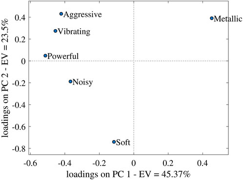
Figure 1. Loadings on the first two Principal Components of the sensory profile (PC1, PC2) for the constant speed condition. Reprinted from: “Sound quality of side-by-side vehicles: Investigation of multidimensional sensory profiles and loudness equalization in an industrial context,” by A. Benghanem et al. (2021) Acta Acustica, 5 (7), page 17. doi: 10.1051/527aacus/2020032 publisher: EDP Sciences.

Figure 2

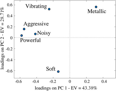
Figure 2. Loadings on the first two Principal Components of the sensory profile (PC1, PC2) for the acceleration condition.

Data from the listening test were global loudness equalized to avoid overestimating loudness in the predictions and to ensure a finer analysis of the timbre structure of the sound for example.

3.1 Predictors

Two families of metrics were used as predictors: 1) physical and psychoacoustic metrics, hereafter referred to as engineering metrics, and 2) the metrics from the MIR (Music Information Retrieval) library used for the extraction of audio and musical characteristics from digital audio files. Among the engineering metrics, the global loudness in sone, the specific loudness on the Bark scale in the 24 frequency bands between 20 Hz and 1,550 Hz, the fluctuation strength, the sound pressure level in dB of the third-octave band spectrum in the 29 frequency bands between 20 Hz and 16,000 Hz, roughness and sharpness were chosen. The MIR metrics used in this research project come from the library MIRtoolbox 1.6.1 for Matlab (Lartillot, 2014). These metrics are grouped into categories: tonality, timbre, rhythm, dynamics, and pitch.

Three statistical variants of each of the metrics were calculated and used as predictors: the mean value over the time duration of the sound sample (Mean), the standard deviation (Std), and the slope over time (Slope). The slope is defined as the linear trend along frames, which is the derivative of the line that best fits the curve. Specifically, the slope $S$ is computed using a normalized representation of the curve $C$—centered, with unit variance, and scaled to a temporal series $T$ of values between 0 and 1. This is solved as a least-squares solution to the equation $S\ast T=C$. The choice of using such metrics is motivated by the need to include significant variables, such as the slope, for acceleration sounds (time-varying signals).

For metric calculation and and their variants, the signal was decomposed into frames, with a frame length of 50 ms and 50% overlap for the MIR metrics, and a 30 ms frame length for the engineering metrics. This frame-based analysis enables the extraction of metrics that are representative of the signal’s composition in both the time and spectral domains, ensuring an accurate capture of its characteristics.

Specific loudness and global loudness values were calculated according to the ISO532B model for stationary sounds (Zwicker et al., 1991) (for constant speed and idle) and according to the model of (Zwicker and Fastl, 1999) for non-stationary sounds (acceleration). Also, the value of the sharpness of a sound, and the value of variable sharpness in time, were calculated according to the procedure proposed by Fastl (derived from Zwicker) with the correction of (Aures, 1985). A total number of 182 metrics (engineering, MIR, including variants for non-stationary signals) were available in the bank of potential model candidates. The temporal variations of the metrics for stationary sounds (idle, constant speed) were then removed, resulting in a total of 127 metrics for these two stationary conditions.

3.2 Lasso and elastic-net

The linear model used to create sound quality models is defined in matrix form and indices:

$v_i={\displaystyle \sum _{m=1}^M}{F}_{im}{b}_m+b+e_i,(1)$

with $v_i$ the ith component of the vector of scores obtained by listening test statistics ($I$ sounds), $F_{im}$ the ith component of the matrix of metrics or scalar measures of $M$ potential predictors for the $I$ sounds, $b_m$ the coefficients to be solved as a vector (linear regression coefficients), $b$ the intercept (the score when all the coefficients $b_m$ are null) and $e_i$ the prediction errors for each ith sound. Equation 1 can be solved using linear regression. In the case of wide data with much fewer observations than predictive metrics $(I<<M)$, classical linear regression based on a least-square approach will typically achieve over-fitting and all the coefficients $b_m$ will be nonzero. As mentioned in the introduction, this strongly limits the interpretation of the resulting model for any engineering use or design guidelines. The aim of the Lasso and Elastic-net is to circumvent this issue by rewriting the problem as a composite cost function (Tibshirani, 1996):

$J_{\lambda ,\alpha }=\frac{1}{2I}\left({\displaystyle \sum _{i=1}^I}{\left(v_i-b-{\displaystyle \sum _{m=1}^M}{b}_m{F}_{im}\right)}^2\right)+\lambda {\displaystyle \sum _{m=1}^M}\left(\frac{\left(1-\alpha \right)}{2}{b}_m^2+\alpha |b_m|\right),(2)$

The first right-hand side term corresponds to the quadratic sum of the predictor errors and the second right-hand side term is a regularization term with regularization amount $\lambda >0$. The regularization combines 2-norm regularization $b_m^2$ and 1-norm regularization $|b_m|$ based on the Elastic-net parameter $0\le \alpha \le 1$. For the Lasso, $\alpha =1$, only the 1-norm regularization is included. This induces solution sparsity, i.e., few coefficients $b_m$ will be non-zero and will be therefore selected in the model (Tibshirani, 1996). The sparsity is controlled by the regularization amount $\lambda$. The Elastic-net (Zou and Hastie, 2005) involves $0<\alpha <1$ and will typically smooth out the selection towards the extreme case of 2-norm-only regularization with $\alpha =0$ (this corresponds to Tikhonov regularization). The minimum of the composite cost function cannot be found by analytical means since it is nonlinear. Therefore, this is solved iteratively using coordinate descent algorithms (Wright, 2015). In Equation 2, $\alpha$ is a user-selected parameter. Note that in the following, to create the simplest and parsimonious models, only the Lasso results are shown $(\alpha =1)$. The penalization amount $\lambda$ is set rigorously using the following procedure: The experimenter defines a limit on the maximum number of metrics that should be included in the model. Here, the aim is to make sure that the model is readable and is meaningful for engineers that can latter use it for product modification. Next, the problem is solved for a wide range of $\lambda$ starting with the largest $\lambda$ so that all coefficients $b_m$ are zeros, and decreasing in successive iterations. The $\lambda$ iteration stops if: 1) the maximum number of non-zero coefficients $b_m$ is reached or 2) the minimum prediction error is obtained for $k$-fold cross-validation of the prediction. Cross-validation is used to avoid overfitting of the model. In this paper, the maximum number of predictive metrics is 7 and the cross-validation is 5-fold.

Cross-validation is a statistical technique used in machine learning and model evaluation. It involves dividing a dataset into subsets, typically a training set to build a predictive model and a validation set to assess its performance. This process is repeated multiple times, each time with a different subset as the validation set and the rest as the training set. The results are then averaged, providing a robust estimate of the model’s performance, helping to mitigate overfitting, and ensuring the model’s generalizability to unseen data. Cross-validation is crucial for selecting the best model and optimizing its hyperparameters while avoiding data leakage and providing a more accurate assessment of predictive performance.

Note that in this study, all seven sounds were retained for the training of the models. While this approach may limit our ability to test the predictive power of the models on new sounds, it is important to highlight that this was not a primary focus or requirement of the study. As a reminder, the main objective of this research is to develop simple objective models that can provide an objective understanding of the measured sounds of side-by-side vehicles. By including all available sounds in the training dataset, we aimed to capture the full range of sound characteristics and ensure a comprehensive analysis within the scope of this study.

4 Results

Tables 1, 2 present the objective models derived from Lasso respectively for the constant speed and the acceleration conditions to predict each perceptual attribute (Powerful, Aggressive, Metallic, Soft, Vibrating, and Noisy), the overall Desire-to-Buy, and the two principal components of the six-dimension sensory profiles of recreational vehicles sounds. The description of the predictors selected in these models can be found in Table 3. Figure 3 presents the listening tests responses and the responses’ prediction of the Powerful attribute for SSV sounds for constant speed condition, as an example.

Table 1

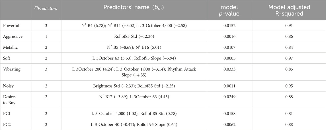
Table 1. Lasso model results for the constant speed condition. The number of predictors selected from the 127 available metrics $(n_{\mathit{Predictors}})$ used to build the Lasso models is shown in the second column. The estimated coefficients $(b_m)$ of each predictor are listed in parenthesis. The description of the predictors can be found in Table 3.

Table 2

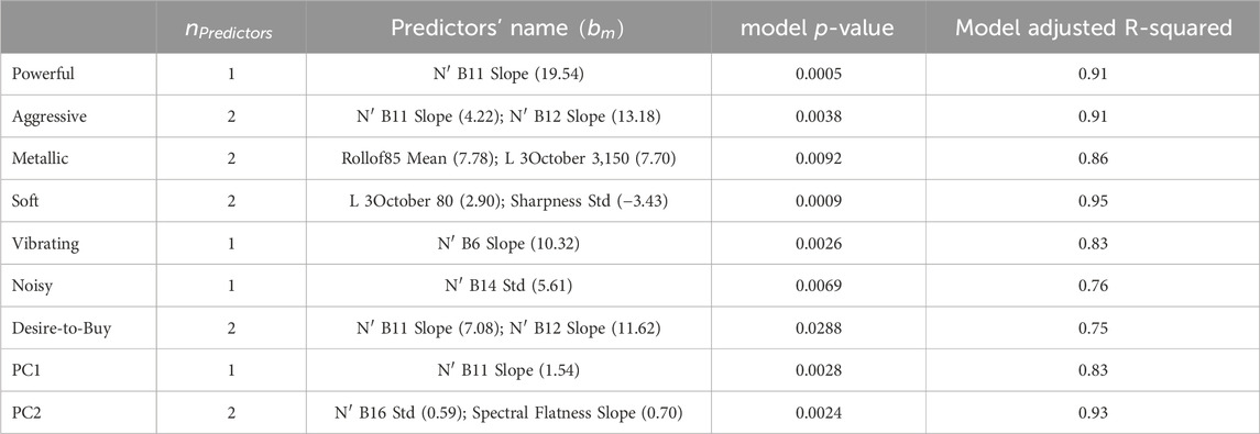
Table 2. Lasso model results for the acceleration condition. The number of predictors selected from the 127 available metrics $(n_{\mathit{Predictors}})$ used to build the Lasso models is shown in the second column. The estimated coefficients $(b_m)$ of each predictor are listed in parenthesis. The description of the predictors can be found in Table 3.

Table 3

Table 3. Description of the predictors used for constructing the Lasso models.

Figure 3

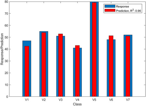
Figure 3. Responses and prediction of responses of the Powerful attribute for SSV sounds for constant speed condition. The thick bars (in blue) indicate the responses and the thinner bars (in red) indicate the model predictions. The horizontal axis labels (V1, V2, etc.) correspond to individual vehicles. The model’s fit, represented by the coefficient of determination $(R^2=0.96)$, is shown in the legend.

4.1 Models’ prediction for the constant speed condition

As can be seen in Table 1, the Lasso models were able to predict the Powerful attribute with a coefficient of determination of 91% using only three predictors, the Aggressive attribute with a coefficient of determination of 86% using only one predictor, the Metallic attribute with a coefficient of determination of 84% using only two predictors, the Soft attribute with a coefficient of determination of 97% using only two predictors, the Vibrating attribute with a coefficient of determination of 85% using only three predictors, the Noisy attribute with a coefficient of determination of 95% using only two predictors, and the overall Desire-to-Buy with a coefficient of determination of 88% using only two predictors. The models derived from Lasso were also able to predict the average scores of PC1 with a coefficient of determination of 81% with only two predictors, and the average scores of PC2 with a coefficient of determination of 88% with only two predictors. All predictors were selected by the Lasso algorithm, which identifies the most relevant metrics (i.e., those that minimize prediction error) from the 127 available, with a maximum of three metrics per model.

The high adjusted coefficients of determination (adjusted $R^2$) and low p-values indicate that each of these models can be considered statistically reliable. Based on the model’s estimated coefficients, the following conclusions can be drawn regarding the constant speed condition:

$•$ Powerful attribute: the specific loudness of Bark 4 positively impacts this model, while the specific loudness of Bark 14 and the level (dB) per 1/3 octave band of the 4,000 Hz band (3,548 Hz–4,467 Hz) negatively impact it. This means that 1) an increase in the energy in this low-frequency range (Bark 4) makes the sound feel more powerful and robust, 2) excessive energy in this higher frequency range (Bark 14) can make the sound feel less powerful, and 3) higher levels of energy in the 4,000 Hz band can reduce the overall sense of power.

$•$ Aggressive attribute: the standard deviation (over time) of the frequency below which 85% of the total energy of the spectrum is contained negatively impacts this model, suggesting that less variation in high-frequency energy correlates with a more aggressive perception of the sound.

$•$ Metallic attribute: the specific loudness of Bark 5 and 16 have opposite impacts on this model. Specifically, to sound more metallic, an SSV sound should have less energy in the Bark 5 band and more energy in the Bark 16 band.

$•$ Soft attribute: the level in dB of the band centered at 63 Hz (56.8 Hz–70.8 Hz) positively impacts this model, while the slope (over time) of the frequency below which 95% of the total energy of the spectrum is contained negatively impacts it. This suggests that higher energy content in the 56.8–70.8 Hz band and a lower Rolloff95 slope correlate with a softer sound.

$•$ Vibrating attribute: the level in dB of the third-octave band centered at 200 Hz (178 Hz–224 Hz) positively impacts this model, while the dB level of the band centered at 1,000 Hz (891 Hz–1,122 Hz) as well as the slope of the rhythm attack negatively impacts it. This suggests that a higher energy content in the 178 Hz–224 Hz band, a lower energy content in the 891 Hz–1,122 Hz band, and a lower slope of attack (lower slope of transient events in the signal, i.e. reduced increase of transient events with time) correlate with a more vibrating sound.

$•$ Noisy attribute: both the standard deviation of the brightness (variation of brightness over time) and the standard deviation (over time) of the frequency below which 85% of the total energy of the spectrum is contained negatively impacts this model. This suggests that lower variation (over time) of the energy in the mid-and high-frequency ranges correlates with a noisier sound.

$•$ Desire-to-buy: the specific loudness of the Bark 17 band (3,150 Hz–3,700 Hz) negatively impacts this model, while the level in dB of the band centered at 63 Hz (56.2 Hz–70.8 Hz) positively impacts it. This suggests an incentive to design SSVs with a sound signature with more emphasis on low frequencies, as these frequencies contribute positively to the desire-to-buy score.

$•$ PC1: Both the level in dB of the band centered at 4,000 Hz (3,548 Hz–4,467 Hz) and the standard deviation of the Spectral Rollof85 metric positively impacts this model. It is noteworthy that these two metrics are also selected by Lasso in the models for the Powerful and Aggressive attributes.

$•$ PC2: the level in dB of the band centered at 40 Hz (35.5 Hz–44.7 Hz) negatively impacts this model, while the slope of the spectral Rollof95 positively impacts it.

4.2 Models’ prediction for the acceleration condition

As can be seen in Table 2, the Lasso models were able to predict the Powerful attribute with a coefficient of determination of 91% using only one predictor, the Aggressive attribute with a coefficient of determination of 91% using only two predictors, the Metallic attribute with a coefficient of determination of 86% using only two predictors, the Soft attribute with a coefficient of determination of 95% using only two predictors, the Vibrating attribute with a coefficient of determination of 83% using only one predictor, the Noisy attribute with a coefficient of determination of 76% using only one predictor, and the overall Desire-to-Buy with a coefficient of determination of 75% using only two predictors. The models derived from Lasso were also able to predict the average scores of PC1 with a coefficient of determination of 83% with only one predictor, and the average scores of PC2 with a coefficient of determination of 93% with only two predictors. Here again, all predictors were selected by the Lasso algorithm, which identifies the most relevant metrics (i.e., those that minimize prediction error) from the 127 available, with a maximum of three metrics per model.

The high adjusted coefficients of determination (adjusted $R^2$) and low p-values indicate that each of these models can be considered statistically reliable. Based on the model’s estimated coefficients, the following conclusions can be drawn regarding the acceleration condition:

$•$ Powerful attribute: the slope (over time) of the specific loudness of Bark 11 positively impacts this model. This suggests that a steady increase in the energy in the Bark 11 band correlates with a more powerful perception of the sound during acceleration. This indicates that an increase in energy over time within this mid-frequency range (Bark 11) contributes to a more powerful and dynamic perception of the sound during acceleration.

$•$ Aggressive attribute: the slope (over time) of the specific loudness of both Bark bands 11 and 12 positively impacts this model. This implies that a steady increase in the energy in these two Bark bands makes the sound of acceleration feel more aggressive.

$•$ Metallic attribute: both the mean of the frequency below which 85% of the total energy of the spectrum is contained and the level in dB of the third-octave band centered at 3,150 Hz positively impacts this model.

$•$ Soft attribute: the standard deviation (over time) of the sharpness negatively impacts this model, while the level in dB of the third-octave band centered at 80 Hz (70.8 Hz–89.1 Hz) positively impacts it. This suggests that a stable sharpness and a pronounced low-frequency content in the 80 Hz band lead to a softer perception of the acceleration sound.

$•$ Vibrating attribute: the slope (over time) of the specific loudness of Bark 6 positively impacts this model. This suggests that a steady increase in the energy of Bark 6 band will make the sound of acceleration feel more vibrating.

$•$ Noisy attribute: the standard deviation (over time) of the specific loudness of Bark 14 positively impacts this model. This implies that greater variation in the loudness of the Bark 14 band correlates with a noisier perception of the acceleration sound.

$•$ Desire-to-buy: the slope (over time) of the specific loudness of both Bark 11 and 12 positively impacts this model. Notably, these two metrics are also selected by Lasso in the models for the Powerful and Aggressive attributes, suggesting that the sound signature of an SSV’s acceleration should “sound” more Powerful and Aggressive to increase the desire to purchase.

$•$ PC1: the slope (over time) of the specific loudness of Bark 11 positively impacts this model.

$•$ PC2: both the standard deviation (over time) of the specific loudness of Bark 16 and the slope of the spectral flatness positively impact this model.

4.3 Interpretation of models

In this study, we were also interested in communicating simply the meaning of the objective models using a simple holistic visual representation.

To this end, Figures 4, 5 present a summary of the sound signature and sound quality models for the constant speed and the acceleration conditions, respectively. These figures provide a visual illustration of the different models for predicting the sound signature and sound quality of SSVs with the metrics selected in each model. These figures also show the effectiveness of the Lasso in selecting only a few metrics to build these parsimonious models from a large metric bank.

Figure 4

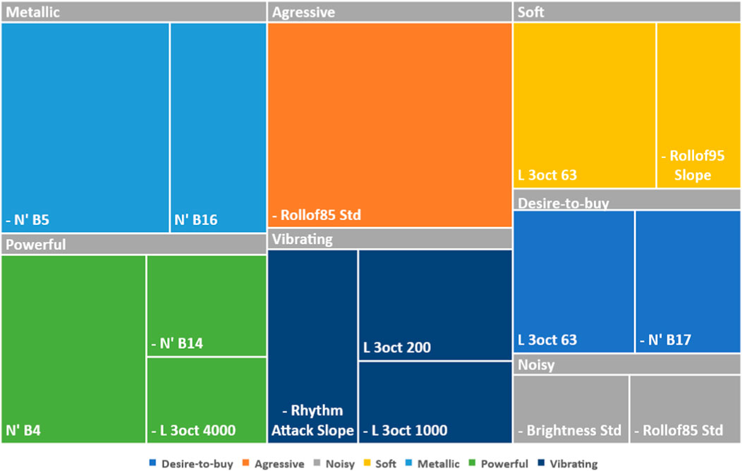
Figure 4. Objective models of SSV sounds for constant speed condition. The colors are associated with the attributes to be predicted. The area of each metric (represented by a rectangle) is relative to its contribution (or coefficient $(b_m)$) in the model. The description of metrics can be found in Table 3. Rectangles are ordered from largest to smallest from left to right and from top to bottom. A minus sign $(-)$ is shown in front of metrics that have a negative coefficient in the model.

Figure 5

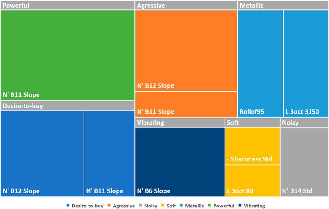
Figure 5. Objective models of SSV sounds for acceleration condition. The colors are associated with the attributes to be predicted. The area of each metric (represented by a rectangle) is relative to its contribution (or coefficient $(b_m)$) in the model. The description of metrics can be found in Table 3. Rectangles are ordered from largest to smallest from left to right and from top to bottom. A minus sign $(-)$ is shown in front of metrics that have a negative coefficient in the model.

From the models developed in this paper, it is now possible to retrieve the sound signature and sound quality of current SSVs and predict those of sounds measured on new SSVs or with virtually modified sounds. However, comparing vehicles based on all these models (all metrics in all three conditions) is likely to be confusing. Therefore, to simplify this, i.e., to make it easier to grasp the contribution of each metric and to compare between sounds, we created a tool named “attribute wheel of SSVs.” This tool allows one to easily visualize the different metrics, their contributions, the corresponding perceptual attributes, and the operating conditions for a given vehicle. It is typically read from the center to the circumference. This wheel of attributes is equivalent to the wine aroma wheel (Noble et al., 1987). As an example, Figure 6 shows the attribute wheel for the second vehicle (named V2 hereafter). The attribute wheel has three levels (the three circular rings in Figure 6):

1. The operational conditions are represented by three different categories: Constant speed (Cst speed), idle, and acceleration. Note that models for the idle condition are not reported in this paper.

2. The scores of the attributes and the Desire-to-buy, represented by the areas of sectors for each attribute. The score values are ordered clockwise from the largest to the smallest value for each condition.

3. The objective metrics retained in the sparse models, represented by sectors of the outer ring. Each attribute is subdivided by the number of retained metrics in the model using the metric coefficients as bin sizes. A minus sign in the metric indicates a negative coefficient of this metric in the model.

Figure 6

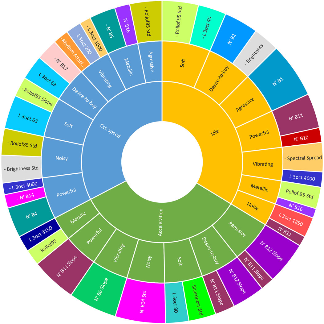
Figure 6. Wheel of attributes for vehicle V2. The attribute scores are ordered for each driving condition from largest to smallest in a clockwise direction. Starting at the center ring with the conditions, we move towards the outer rings, with attributes in the second ring and metrics in the last ring. The size of each metric is relative to its contribution in the model. The description of metrics can be found in Table 3. In the third ring, the colors assigned to the metrics do not carry any specific meaning. They are solely added to differentiate between the metrics visually. The purpose of using different colors is to aid in the visual distinction and organization of the metrics within the model. It is important to note that the colors do not convey any additional information or signify any particular significance or relationship among the metrics.

For instance, for the acceleration condition of V2, shown in Figure 6, the Aggressive attribute has the largest score compared to the other attributes. The Aggressive objective model involves the two metrics N′ B12 Slope and N′ B11 Slope. These two metrics are the band-specific loudness slopes of Bark bands 11 and 12 (1,270 Hz–1720 Hz), respectively. This result suggests that the aggressiveness of the acceleration sound is predicted by the time variation of the spectral content in these two Bark bands. The graph also suggests that the effect of the N′ B12 Slope predictor is much larger than the N′ B11 Slope predictor in the model. The graph also shows that the same two metrics are involved in the Desire-to-buy objective model for this condition. Therefore, any positive variation in these two metrics will result in positive variations of the Aggressive attribute and Desire-to-buy. The inclusion of Desire-to-buy as one of the perceptual attributes in Figure 6 may seem odd. Specifically, in the idle condition, the features selected for the Desire-to-buy model do not match those of any of the perceptual attribute models. However, it should be noted that the idle condition may not be as critical in influencing the overall “desire to purchase” factor as the acceleration condition. Interestingly, in the acceleration condition, the two parameters used in the Desire-to-buy model are identical to those of the Aggressive perceptual attribute. This observation suggests a potential correlation between the perception of aggressiveness and the Desire-to-buy during acceleration, which could be a valuable element for further study.

5 Discussion

The results show that the Lasso can select a few significant metrics from a large bank of metrics for the objective models of subjective assessments of SSV sounds. Indeed, when generating models (of sensory profiles, sound quality, and principal components of the sensory attributes), the Lasso retained only one, two, or three predictors at most in each model from a list of 127 potential predictors (182 predictors for rapid acceleration), leading to parsimonious and easily understandable models.

Overall, the objective model for Desire-to-buy suggests designing SSVs with a sound signature that emphasizes low frequencies. Also, since the acceleration condition (non-stationary signals) is important for the global sound quality of SSVs, the objective models should include time variation properties of the related signals and not just the time-averaged values.

For the reported data, the constructed models have good consistency and statistical significance. However, since the number of samples in the cross-validation data was small, the significance of these models for new sounds (samples that are distinct from the sounds used in the listening tests) needs to be investigated.

In this study, we also propose a graphical visualization tool (attribute wheel of SSVs) to easily interpret the objective models of the sound signature and sound quality of SSVs. For instance, on practical grounds, this resulted in useful indications for sound quality optimization and for adjusting the sound signature of the SSVs for the industrial partner that pursues the constant amelioration of the sound of the SSVs.

6 Conclusion

The goal of this study was to develop objective models of subjective assessments of SSV sounds. The applications of these models being, first the prediction of sound quality of side-by-side vehicles (SSV), and second, the explanation of the underlying structure of perceived sound quality of SSV to guide engineers in future design (i.e. increase this sound, reduce the brightness, etc.). This paper has provided a set of experimental results that allow a better understanding of the sensory profiles and sound quality of SSVs using physical and psychoacoustic metrics. When generating the models, the Lasso retained only a few significant metrics in each model from a large number of potential predictors, which led to parsimonious and easily interpretable models. In addition, a graphical tool for visualizing the metrics, named “attribute wheel of SSVs,” was developed as part of this study. It facilitates the interpretation of the contributions of metrics in models on the overall sound quality of SSVs. This has led to useful insights for sound quality optimization and for adjusting the sound signature of SSVs in general and the studied vehicle in particular. Using such illustrations and models, acoustic engineers from the SSV manufacturer can adjust future designs for a stronger desirability or a better sensory profile of SSVs.

Data availability statement

The raw data supporting the conclusions of this article will be made available by the authors, without undue reservation.

Ethics statement

The studies involving humans were approved by CER Lettre et sciences humaines, Université de Sherbrooke. The studies were conducted in accordance with the local legislation and institutional requirements. The participants provided their written informed consent to participate in this study.

Author contributions

AB: Conceptualization, Data curation, Formal Analysis, Investigation, Methodology, Project administration, Resources, Software, Validation, Visualization, Writing–original draft, Writing–review and editing. OV: Conceptualization, Data curation, Formal Analysis, Investigation, Methodology, Project administration, Resources, Software, Validation, Visualization, Writing–original draft, Writing–review and editing. P-AG: Conceptualization, Funding acquisition, Project administration, Supervision, Writing–original draft, Writing–review and editing. AB: Conceptualization, Funding acquisition, Project administration, Supervision, Writing–original draft, Writing–review and editing.

Funding

The author(s) declare that financial support was received for the research, authorship, and/or publication of this article. The authors wish to acknowledge the financial support from the “Natural Sciences and Engineering Research Council of Canada” (NSERC), “Bombardier Recreational Products” (BRP) and the “Centre de Technologies Avancées BRP-UdeS” (CTA).

Acknowledgments

The authors wish to acknowledge the technical support provided by the members of the dXBel project. The authors would like to thank Paul Massé from the BRP marketing group for moderating the group discussions and for his support as well as all participants who completed the subjective experiments described in this paper. The data collection with human subjects was approved by the ethical committee CÉR - Lettres et sciences humaines of Université de Sherbrooke (#2017-1546).

Conflict of interest

The authors declare that the research was conducted in the absence of any commercial or financial relationships that could be construed as a potential conflict of interest.

Publisher’s note

All claims expressed in this article are solely those of the authors and do not necessarily represent those of their affiliated organizations, or those of the publisher, the editors and the reviewers. Any product that may be evaluated in this article, or claim that may be made by its manufacturer, is not guaranteed or endorsed by the publisher.

References

Aures, W. (1985). ‘berechnungsverfahren für den sensorischen wohlklang beliebiger schallsignale’ (a model for calculating the sensory euphony of various sounds). Acustica 59.

Google Scholar

Benghanem, A., Valentin, O., Gauthier, P.-A., and Berry, A. (2021). Sound quality of side-by-side vehicles: Investigation of multidimensional sensory profiles and loudness equalization in an industrial context. Acta Acust. 5, 7. Publisher: EDP Sciences. doi:10.1051/aacus/2020032

CrossRef Full Text | Google Scholar

Chen, P., Xu, L., Liu, W., and Shang, L. (2022). Research on prediction model of tractor sound quality based on genetic algorithm. Appl. Acoust. 185, 108411. doi:10.1016/j.apacoust.2021.108411

CrossRef Full Text | Google Scholar

Chen, S., and Wang, D. (2014). Vehicle interior sound quality analysis by using grey relational analysis. SAE Int. J. Passeng. Cars Mech. Syst. 7, 355–366. doi:10.4271/2014-01-1976

CrossRef Full Text | Google Scholar

Choi, K., Fazekas, G., Cho, K., and Sandler, M. B. (2017). A tutorial on deep learning for music information retrieval. Corr. abs/1709, 04396.

Google Scholar

Downie, J. S. (2003). Music information retrieval. Annu. Rev. Inf. Sci. Technol. 37, 295–340. doi:10.1002/aris.1440370108

CrossRef Full Text | Google Scholar

Fastl, H., and Zwicker, E. (2007). Psychoacoustics: facts and models. 22. Berlin and Heidelberg: Springer.

Google Scholar

Friedman, J., Hastie, T., and Tibshirani, R. (2010). A note on the group lasso and a sparse group lasso

Google Scholar

Gauthier, P.-A., Scullion, W., and Berry, A. (2017). Sound quality prediction based on systematic metric selection and shrinkage: comparison of stepwise, lasso, and elastic-net algorithms and clustering preprocessing. J. Sound Vib. 400, 134–153. doi:10.1016/j.jsv.2017.03.025

CrossRef Full Text | Google Scholar

Huang, H., Wu, J., Ding, W., and Yang, M. (2021). Pure electric vehicle nonstationary interior sound quality prediction based on deep cnns with an adaptable learning rate tree. Mech. Syst. Signal Process. 148, 107170. doi:10.1016/j.ymssp.2020.107170

CrossRef Full Text | Google Scholar

Huang, X., Huang, H., Wu, J., Yang, M., and Ding, W. (2020). Sound quality prediction and improving of vehicle interior noise based on deep convolutional neural networks. Expert Syst. Appl. 160, 113657. doi:10.1016/j.eswa.2020.113657

CrossRef Full Text | Google Scholar

Jiang, J., and Zeng, Y. (2014). Subjective and objective quantificational description of vehicle interior noise during acceleration. Appl. Mech. & Mater. 518, 297–302. doi:10.4028/www.scientific.net/amm.518.297

CrossRef Full Text | Google Scholar

Kim, T. G., Lee, S.-K., and Lee, H. H. (2009). Characterization and quantification of luxury sound quality in premium-class passenger cars. Proc. Institution Mech. Eng. – Part D – J. Automob. Eng. 223, 343–353. doi:10.1243/09544070jauto989

CrossRef Full Text | Google Scholar

Kwon, G., Jo, H., and Kang, Y. J. (2018). Model of psychoacoustic sportiness for vehicle interior sound: excluding loudness. Appl. Acoust. 136, 16–25. doi:10.1016/j.apacoust.2018.01.027

CrossRef Full Text | Google Scholar

Lartillot, O. (2014). MIRtoolbox 1.6.1. User’s manual. Denmark: Aalborg University.

Google Scholar

Lee, S.-K. (2008). Objective evaluation of interior sound quality in passenger cars during acceleration. J. Sound Vib. 310, 149–168. doi:10.1016/j.jsv.2007.07.073

CrossRef Full Text | Google Scholar

Lyon, R. (2003). An introduction to sound quality. J. Sound Vib. 6, 6.

Google Scholar

Noble, A., Arnold, R., Buechsenstein, J., Leach, E., Schmidt, J., and Stern, P. (1987). Modification of a standardized system of wine aroma terminology. Am. J. Enol. Vitic. 38, 143–146. doi:10.5344/ajev.1987.38.2.143

CrossRef Full Text | Google Scholar

Otto, N., Amman, S., Eaton, C., and Lake, S. (2001) “Guidelines for jury evaluations of automotive sounds,” in Sound and vibration, 1–14.

Google Scholar

Paulraj, P., Melvin, A. A., and Sazali, Y. (2013). Car cabin interior noise classification using temporal composite features and probabilistic neural network model. Appl. Mech. Mater. 471, 64–68. doi:10.4028/www.scientific.net/amm.471.64

CrossRef Full Text | Google Scholar

Rumsey, F. (2009). Searching, analyzing, and recommending audio content. JAES 57, 166–169.

Google Scholar

Tibshirani, R. (1996). Regression shrinkage and selection via the lasso. J. R. Stat. Soc. Ser. B Methodol. 58, 267–288. doi:10.1111/j.2517-6161.1996.tb02080.x

CrossRef Full Text | Google Scholar

Tibshirani, R. J., and Taylor, J. (2011). The solution path of the generalized lasso. Ann. Statistics 39, 1335–1371. doi:10.1214/11-aos878

CrossRef Full Text | Google Scholar

Urbano, M. S., and Serra, X. (2013). Evaluation in music information retrieval. J. Intell. Inf. Syst. 41, 345–369. doi:10.1007/s10844-013-0249-4

CrossRef Full Text | Google Scholar

Wang, Y., Shen, G., and Xing, Y. (2014). A sound quality model for objective synthesis evaluation of vehicle interior noise based on artificial neural network. Mech. Syst. Signal Process. 45, 255–266. doi:10.1016/j.ymssp.2013.11.001

CrossRef Full Text | Google Scholar

Wright, S. (2015). Coordinate descent algorithms. Math. Program 151, 3–34. doi:10.1007/s10107-015-0892-3

CrossRef Full Text | Google Scholar

Xiong, T., Bao, Y., and Chiong, R. (2015). Forecasting interval time series using a fully complex-valued rbf neural network with dpso and pso algorithms. Inf. Sci. 305, 77–92. doi:10.1016/j.ins.2015.01.029

CrossRef Full Text | Google Scholar

Zhekova, I. (2007). Analyse temps-fréquence et synthèse granulaire des bruits moteur diesel au ralenti: Application pour étude perceptive dans le contexte des scènes auditives. Marseille, France.

Google Scholar

Zou, H., and Hastie, T. (2005). Regularization and variable selection via the elastic net. J. R. Stat. Soc. Ser. B Stat. Methodol. 67, 301–320. doi:10.1111/j.1467-9868.2005.00503.x

CrossRef Full Text | Google Scholar

Zwicker, E., and Fastl, H. (1999). Psychoacoustics: facts and models. 2 edn. Berlin: Springer-Verlag.

Google Scholar

Zwicker, E., Fastl, H., Widmann, U., Kurakata, K., Kuwano, S., and Namba, S. (1991). Program for calculating loudness according to din 45631 (ISO532B). J. Acoust. Soc. Jpn. (E) 12, 39–42. doi:10.1250/ast.12.39

CrossRef Full Text | Google Scholar