On the use of the local reflection coefficient to assess the diffuse field sound absorption coefficient of a porous material

The diffuse field sound absorption coefficient (SAC) of a sound absorber can be obtained from an average over the incidence angles of the oblique incidence plane wave SAC. The plane wave SAC can be derived from the plane wave complex-valued reflection coefficient defined as the ratio of the reflected sound pressure at a given point on the material surface to the incident sound pressure at the same point. In practice, the material is excited by a monopole, and the reflection coefficient becomes a local quantity which is a function of the source height and the radial distance from the source. This local reflection coefficient obtained at various points on the material surface is commonly used to approximate the oblique incidence plane wave reflection coefficient. The error in estimating the diffuse field SAC introduced by this approximation has not been explored in the literature. This paper investigates this error as a function of the material extent, thickness, and source height using an analytical approach to calculate the local reflection coefficient. The calculation is based on Allard’s model which describes the sound propagation above an infinite lateral extent porous material backed by a rigid wall and excited by a monopole. Using finite element simulations as a reference, the analytical model is shown to provide a good approximation of the diffuse field sound absorption performance of sufficiently large material areas. The diffuse field SAC calculated from plane wave reflection coefficients and local reflection coefficient are compared. The limitations inherent in deriving diffuse field SACs from local reflection measurements obtained with a monopole are highlighted.

1 Introduction

One of the key metrics used in evaluating and comparing materials’ sound absorption capabilities is the Sound Absorption Coefficient (SAC). SACs depend on the nature of the incident sound field. Typically, idealized incident fields such as diffuse field and normal or oblique incidence plane waves are employed in practical assessments.

For a homogeneous material with infinite lateral extent excited by an oblique incidence plane wave at an incidence angle $\theta$, the SAC—denoted as ${\alpha }_{\text{pw}}\left(\theta ,\omega \right)$—can be determined using the complex-valued reflection coefficient—denoted as $\widehat{\mathfrak{R}}\left(\theta ,\omega \right)$—where $\omega$ represents the angular frequency. $\widehat{\mathfrak{R}}\left(\theta ,\omega \right)$ is defined as the complex-valued ratio of the reflected sound pressure at a specific point on the material surface to the incident sound pressure at the same point. This coefficient is intricately linked to the material surface impedance ${\widehat{Z}}_s$ (Pierce, 1989). ${\alpha }_{\text{pw}}\left(\theta ,\omega \right)$ can then be obtained from the relationship ${\alpha }_{\text{pw}}\left(\theta ,\omega \right)=1-{\left|\widehat{\mathfrak{R}}\left(\theta ,\omega \right)\right|}^2$. In the scenario of a plane wave and homogeneous material, the reflection coefficient (and thus the SAC) remains independent of the position of the point on the material surface. The diffuse field SAC can be derived from an averaging process over the incidence angles of ${\alpha }_{\text{pw}}\left(\theta ,\omega \right)$ (Allard and Atalla, 2009).

In practical applications, the material is excited by a monopole, and the reflection coefficient, denoted as ${\widehat{\mathfrak{R}}}_{\mathit{l}\mathit{o}\mathit{c}}\left(\mathit{r},{\mathit{z}}_{\mathit{s}},\mathit{\omega }\right)$, is a local quantity (Nobile, 2005; Dragonetti and Romano, 2015; Dragonetti et al., 2016) influenced by the source height ${\mathrm{z}}_{\mathrm{s}}$ and radial distance $\mathrm{r}$ from the source. This local reflection coefficient ${\widehat{\mathfrak{R}}}_{\mathit{l}\mathit{o}\mathit{c}}\left(\mathit{r},{\mathit{z}}_{\mathit{s}},\mathit{\omega }\right)$, measured at different points on the material surface, is commonly utilized to approximate $\widehat{\mathfrak{R}}\left(\mathit{\theta },\mathit{\omega }\right)$. In this context, $\mathrm{\theta }$, determined by ${\mathit{z}}_{\mathit{s}}$ and $\mathit{r}$, represents the angle between the normal to the material surface and the line connecting the source position to the point of interest on the material surface. An associated local sound absorption coefficient, ${\alpha }_{l\text{oc}}\left(r,z_s,\omega \right)$, can then be calculated. ${\alpha }_{l\text{oc}}\left(r,z_s,\omega \right)$ may exhibit significant variation across the material surface and is influenced by material dimensions as well as the incident wave-front impinging upon it (Dragonetti and Romano, 2015).

${\widehat{\mathfrak{R}}}_{l\text{oc}}\left(r,z_s,\omega \right)$, or equivalently ${\widehat{\mathfrak{R}}}_{l\text{oc}}\left(\theta ,z_s,\omega \right)$ since ${r=z}_s\tan \theta$, is typically estimated using a microphone doublet positioned at a short distance from the material. Implicit in this process is the assumption that, locally, the incident and reflected fields demonstrate characteristics similar to a plane wave. Once ${\widehat{\mathfrak{R}}}_{l\text{oc}}\left(\theta ,z_s,\omega \right)$ has been determined for multiple incidences by varying the measurement point along the material surface and subsequently substituted for $\widehat{\mathfrak{R}}\left(\theta ,\omega \right)$, the diffuse field SAC can be obtained by averaging ${\alpha }_{\text{pw}}\left(\theta ,\omega \right)$ over the various incidence angles.

Alternatively, based on reciprocity and assuming that the material is homogeneous, ${\widehat{\mathfrak{R}}}_{l\text{oc}}\left(\theta ,z_s,\omega \right)$ values measured with a microphone doublet above the material surface for a monopole source moved at various positions (synthetic array) in free-field conditions can be utilized in a synthesis method to retroactively compute the SAC for any incident sound field, particularly a diffuse field (Robin et al., 2014; 2019). Although the approximation of $\widehat{\mathfrak{R}}\left(\theta ,\omega \right)$ by ${\widehat{\mathfrak{R}}}_{l\text{oc}}\left(\theta ,z_s,\omega \right)$ introduces a degree of error, the conditions under which the error in estimating the diffuse field SAC from ${\widehat{\mathfrak{R}}}_{l\text{oc}}\left(\theta ,z_s,\omega \right)$ is minimized (taking into account the effect of material size, thickness, and/or source height) have not been thoroughly explored in the literature.

Another approach to estimating the SAC of an absorber is to directly use a power-based definition. In this regard, the SAC can be defined as the ratio of the sound power absorbed by a given area of the material to the incident sound power flowing through the same area. This definition, utilizing an area-averaged SAC, provides a more representative estimate for the overall surface (Kuipers et al., 2012, 2014). Recently, the area-averaged effective SAC of a rigid-backed homogeneous porous material subjected to a monopole excitation—referred to as ${\alpha }_{\text{mon}}$—has been investigated using both analytical and finite element models (Sgard et al., 2024). The impact of factors such as source height, material lateral extent, and material characteristics (thickness and acoustical properties) on ${\alpha }_{\text{mon}}$ have been highlighted. It has been demonstrated that the sound absorption performance of porous materials under monopole excitation significantly differs from that observed under plane wave and diffuse field excitations, especially at low frequencies when the source is in close proximity to the material. It should be noted that unlike SAC derived from the local reflection coefficient which can be measured using a microphone doublet, assessing ${\alpha }_{mon}$ requires either the measurement of sound powers (Kuipers et al., 2014, 2012) or the estimation of the complex effective density and wave number either through direct measurement (Allard et al., 1992) or use of a model (e.g., Johnson-Champoux-Allard (JCA)) linking these variables with porous material intrinsic parameters which can themselves be determined using various techniques (Allard and Atalla, 2009). The area-averaged effective SAC is an interesting indicator for assessing the overall sound absorption performance of the material.

This study is fully based on theoretical and numerical models. Its objective is to investigate the extent to which the diffuse field SAC of a porous material, ${\alpha }_{\mathrm{d},\text{loc}}$, can approximate the traditional diffuse field SAC, referred to as ${\alpha }_{\mathrm{d}}$, calculated from plane wave reflection coefficients. With the assumption of sufficiently large finite size materials, the investigation relies on Allard’s model (Allard et al., 1992) to describe the sound propagation above the porous material. This model also allows fast calculations for parametric studies. For small finite size materials whose sound absorption performance is affected by lateral boundary conditions, ${\alpha }_{\mathrm{d},\text{loc}}$ can be calculated alternatively using a numerical method such as the finite element (FE) approach. This numerical approach serves as a reference solution to verify the results of the proposed analytical model and allows one to establish the limits of the analytical model by discussing the effect on ${\alpha }_{\mathrm{d},\text{loc}}$ of the material finite size along with its associated boundary conditions.

The paper is organized as follows. Section 2 presents the theoretical developments for calculating the SAC based on Allard’s model for the sound propagation above a rigid-frame, infinite-lateral-extent porous material excited by a monopole. Next, common definitions of the SAC based on plane wave and diffuse field excitations are recalled. In Section 3, the SAC ${\alpha }_{\mathrm{d},\text{loc}}$ calculated from Allard’s model is verified using a numerical finite element (FE) approach. Then, the capability of the analytical model to provide SAC values for porous material samples of finite size is assessed by comparing them with FE calculations across various sizes, thicknesses, and boundary conditions. Furthermore, numerical comparisons between ${\alpha }_{\mathrm{d},\text{loc}}$ and ${\alpha }_{\mathrm{d}}$, for different monopole heights, material lateral extents, and material thicknesses are conducted to assess associated errors. Section 3 concludes with a discussion on the limitations of the study, while Section 4 outlines its conclusions.

2 Materials and methods

2.1 Allard’s model

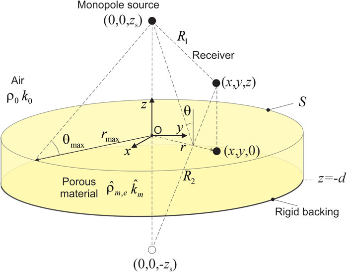
In the following, the convention $p\left(r,z,t\right)=\mathfrak{R}\left[\widehat{p}\left(r,z,\omega \right)e^{j\omega t}\right]$ is used where $\widehat{p}$ denotes the complex sound pressure, ${\widehat{p}}^{*}$, $\mathfrak{R}\left[\widehat{p}\right],\mathfrak{I}\left[\widehat{p}\right]$ and $\left|\widehat{p}\right|$ denote its complex conjugate, real part, imaginary part and absolute value, respectively. $\overline{a\left(t\right)}$ denotes the time average over a period of the time dependent quantity $a\left(t\right)$. Assuming cylindrical symmetry, we consider a monopole of volume flow rate $\widehat{Q}$ located at $\left(0,0,z_s\right)$ in a fluid of density ${\rho }_0$ and sound speed $c_0$ above a porous material cylindrical sample of radius $r_{\max }\text{\hspace{0.17em}and\hspace{0.17em}thickness\hspace{0.17em}}d$ of porosity $\varphi$ backed by a rigid surface (Figure 1).

Figure 1

Figure 1. Description of the problem of interest.

The porous material should behave as an equivalent fluid of complex equivalent density ${\widehat{\rho }}_m$ (effective density ${\widehat{\rho }}_{m,e}=\frac{{\widehat{\rho }}_m}{\varphi }$) and wave number ${\widehat{k}}_m$. For a material of infinite lateral extent ($r_{\max }\to \infty$), the sound pressure at any point above the porous material is given by (Thomasson, 1977; Allard et al., 1992):

$\widehat{p}\left(r,z,\omega \right)=j{\rho }_0\omega \widehat{Q}\left(\frac{e^{-j{k}_0{R}_1}}{R_1}-\frac{e^{-j{k}_0{R}_2}}{R_2}+{\int }_0^{+\infty }\frac{2{\widehat{\rho }}_{m,e}}{{\widehat{\rho }}_{m,e}{\widehat{\nu }}_0+{\rho }_0{\widehat{\nu }}_m\tanh \left({\widehat{\nu }}_{m}d\right)}{e}^{-{\widehat{\nu }}_0\left(z_s+z\right)}{J}_0\left(r{k}_r\right)k_{r}d{k}_r\right)(1)$

where $r=\sqrt{x^2+y^2}$ is the radial distance between the source and the receiver and $z$ denotes the vertical distance between the point of interest and the material surface. $J_0$ is the zeroth-order Bessel function. In addition, $R_1=\sqrt{r^2+{\left(z_s-z\right)}^2}$, $R_2=\sqrt{r^2+{\left(z_s+z\right)}^2}$, ${\widehat{\nu }}_0^2=k_r^2-k_0^2$, ${\widehat{\nu }}_m^2=k_r^2-{\widehat{k}}_m^2$. $k_0$ is the wave number in air, and $k_r$ refers to a radial wave number. For the receiver $\left(r,z\right)$, an incidence angle $\theta$ can be defined (Figure 1). Eq. 1 can also be rewritten as

$\widehat{p}\left(r,z,\omega \right)={\widehat{p}}_{inc}\left(r,z,\omega \right)+{\widehat{p}}_{ref}\left(r,z,\omega \right)(2)$

where

${\widehat{p}}_{inc}\left(r,z,\omega \right)=j{\rho }_0\omega \widehat{Q}\frac{e^{-j{k}_0{R}_1}}{R_1}(3)$

is the incident sound pressure field and ${\widehat{p}}_{ref}\left(r,z,\omega \right)$ is the reflected sound pressure field given by:

${\widehat{p}}_{ref}\left(r,z,\omega \right)=j{\rho }_0\omega \widehat{Q}\left(-\frac{e^{-j{k}_0{R}_2}}{R_2}+{\int }_0^{+\infty }\frac{2{\widehat{\rho }}_{m,e}}{{\widehat{\rho }}_{m,e}{\widehat{\nu }}_0+{\rho }_0{\widehat{\nu }}_m\tanh \left({\widehat{\nu }}_{m}d\right)}{e}^{-{\widehat{\nu }}_0\left(z_s+z\right)}{J}_0\left(r{k}_r\right)k_{r}d{k}_r\right)(4)$

2.2 Calculation of the SAC

2.2.1 Oblique incidence—Plane wave excitation

The oblique incidence plane reflection coefficient for a given incidence angle $\theta$ can be computed from the material surface impedance ${\widehat{Z}}_s\left(\theta ,\omega \right)$ by:

$\widehat{\mathfrak{R}}\left(\theta ,\omega \right)=\frac{{\widehat{Z}}_s\left(\theta ,\omega \right)\cos \theta -Z_0}{{\widehat{Z}}_s\left(\theta ,\omega \right)\cos \theta +Z_0}(5)$

where $Z_0$ is the acoustic characteristic impedance of air. For an equivalent fluid of thickness $d$ with a rigid backing,

${\widehat{Z}}_s\left(\theta ,\omega \right)=-j{\widehat{Z}}_{c,m}\left(\omega \right)\frac{{\widehat{k}}_m\cot \left(d\sqrt{{\widehat{k}}_m^2-k_0^2{\sin }^2\theta }\right)}{\varphi \sqrt{{\widehat{k}}_m^2-k_0^2{\sin }^2\theta }}(6)$

with ${\widehat{Z}}_{c,m}$ the characteristic impedance of the material given by ${\widehat{Z}}_{c,m}=\omega \varphi \frac{{\widehat{\rho }}_{m,e}}{{\widehat{k}}_m}$. The oblique incidence plane wave SAC is then given by:

${\alpha }_{\text{pw}}\left(\theta ,\omega \right)=1-{\left|\widehat{\mathfrak{R}}\left(\theta ,\omega \right)\right|}^2(7)$

2.2.2 Oblique incidence—monopole excitation

For a monopole excitation, the local sound absorption coefficient can be computed from the local reflection coefficient referred to as ${\widehat{\mathfrak{R}}}_{l\text{oc}}\left(\theta ,z_s,\omega \right)={\widehat{\mathfrak{R}}}_{\text{loc}}\left(r,z_s,\omega \right)$ given by the ratio of ${\widehat{p}}_{ref}\left(r,0,\omega \right)$ and ${\widehat{p}}_{inc}\left(r,0,\omega \right)$:

${\alpha }_{\text{loc}}\left(\theta ,z_s,\omega \right)=1-{\left|{\widehat{\mathfrak{R}}}_{\text{loc}}\left(\theta ,z_s,\omega \right)\right|}^2(8)$

with $\tan \theta =\frac{r}{z_s}$. In this study, ${\widehat{p}}_{inc}\left(r,0,\omega \right)$ and ${\widehat{p}}_{ref}\left(r,0,\omega \right)$ are calculated using Eqs. 3 and 4 respectively, assuming that ${\widehat{\rho }}_{m,e}$ and ${\widehat{k}}_m$ are known. It is important to recall that Eq. 8 assumes that, locally, the incident and reflected fields demonstrate characteristics similar to a plane wave. When this assumption fails, this expression needs to be revisited (see e.g., Sgard et al. (2024)). In an experimental framework, ${\widehat{\mathfrak{R}}}_{\mathrm{l}\text{oc}}\left(\mathrm{\theta },{\mathrm{z}}_{\mathrm{s}},\mathrm{\omega }\right)$ is typically estimated from the transfer function between two microphones (microphone doublet) located at a short distance from the material surface (Robin et al., 2014; 2019). This microphone doublet approach allows for separation of the incident sound pressure from the reflected one without any need to know ${\widehat{\mathit{\rho }}}_{\mathit{m},\mathit{e}}$ and ${\widehat{\mathit{k}}}_{\mathit{m}}$. It is worth noting that, using reciprocity, the local reflection coefficient ${\widehat{\mathfrak{R}}}_{\text{loc}}\left(r,z_s,\omega \right)$ can be obtained by keeping the receiver at a fixed position and varying the source position or keeping the source at a fixed location and changing the receiver position. Note that by using the stationary phase approximation, Eq. 3 reduces to the plane wave case when $\left|{\widehat{\nu }}_0{z}_s\right|$ becomes large (Allard and Atalla, 2009).

2.2.3 Diffuse field

The diffuse field (or random incidence) SAC can be obtained from the oblique incidence plane wave SAC by Paris (1928):

${\alpha }_{\mathrm{d}}\left({\theta }_{\max },\omega \right)=\frac{{\int }_0^{{\theta }_{\max }}{\alpha }_{\text{pw}}\left(\theta ,\omega \right)\cos \theta \sin \theta d\theta }{{\int }_0^{{\theta }_{\max }}\cos \theta \sin \theta d\theta }(9)$

where ${\alpha }_{\text{pw}}\left(\theta \right)$ is obtained by Eq. 7. ${\theta }_{\max }$ is theoretically equal to ${90}^{\circ }$. In practical applications, as is common for sound transmission loss (Hopkins, 2007; Bies and Hansen, 2014), smaller empirical values (typically ${78}^{\circ }$) can be used for better correlations between predictions and field or laboratory measurements (field incidence). In addition, it is notable that when the diffuse field SAC is calculated using field synthesis approaches based on an array of monopoles above a lateral finite size material (e.g., of radius $r_{\max }$) and a fixed microphone doublet (referred to as ${\alpha }_{\text{synth}}$), better agreement between ${\alpha }_{\text{synth}}$ and ${\alpha }_{\mathrm{d}}$ is achieved when values of ${\theta }_{\max }$ corresponding to the largest incidence angle in Eq. 9 are selected (Robin et al., 2019). This incidence angle is determined from the size and the height of the array and is related to the solid angle that the array subtends from the microphone doublet position.

Alternatively, the diffuse field SAC of a material sample of radius $r_{\max }$ can be approximated in terms of the local reflection coefficient ${\widehat{\mathfrak{R}}}_{\text{loc}}\left(\theta ,z_s,\omega \right)$ obtained for a monopole excitation (height $\left.z_s\right)$ at various angles $\theta$ (or equivalently at various radial distances on the material surface):

$\begin{array}{c}{\alpha }_{\mathrm{d},\text{loc}}\left({\theta }_{\max },z_s,\omega \right)=\frac{{\int }_0^{{\theta }_{\max }}{\alpha }_{\text{loc}}\left(\theta ,z_s,\omega \right)\cos \theta \sin \theta d\theta }{{\int }_0^{{\theta }_{\max }}\cos \theta \sin \theta d\theta }\\ =2\left(\frac{z_s^2}{r_{\max }^2}+1\right){\int }_0^{r_{\max }}\left(1-{\left|{\widehat{\mathfrak{R}}}_{\text{loc}}\left(r,z_s,\omega \right)\right|}^2\right)\frac{z_s^{2}r}{{\left(z_s^2+r^2\right)}^2}dr\end{array}(10)$

which constitutes an approximation of the diffuse field sound absorption coefficient calculated from Eq. 9. In Eq. 10, the value of ${\theta }_{\max }$ has been obtained from the solid angle that the material subtends from the source position (see Figure 1) — $\tan {\theta }_{\max }=\frac{r_{\max }}{z_s}$. This angle corresponds to the maximum incidence angle achievable for a sample of radius $r_{\max }$ excited by a monopole of height $z_s.$ It is important to note that ${\alpha }_{\mathrm{d},\text{loc}}$ is an approximate effective SAC indicator, not a power-based area-averaged effective SAC (Kuipers et al., 2012; 2014; Sgard et al., 2024). It can thus yield anomalous and counterintuitive SAC values (including negative values) when the plane wave approximation fails to hold.

In the above equations, all the integrals are computed numerically using a vectorized adaptive quadrature method (integral Matlab R2023b^® Mathworks routine for 1D-integrals and integral2 for 2-D integrals) (Shampine, 2008).

3 Results and discussion

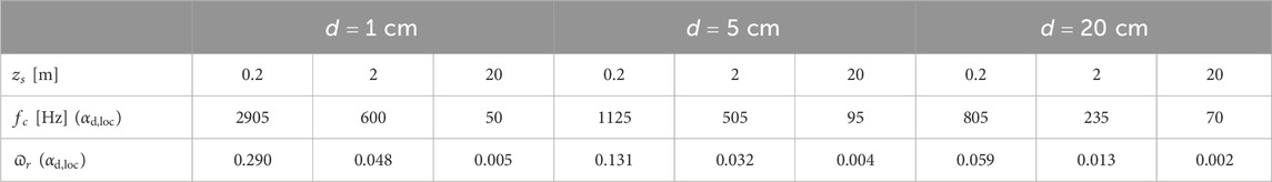
The different models previously presented utilize the complex effective density ${\widehat{\rho }}_{m,e}$ and wave number ${\widehat{k}}_m$, which are determined using the Johnson–Champoux–Allard (JCA) equivalent fluid model (Allard and Atalla, 2009). The five macroscopic parameters necessary for this model were measured at the GRAM-ICAR laboratory at the École de Technologie Supérieure (Montreal, Canada) using conventional direct characterization apparatus (porosimeter, tortuosimeter, and resistivity meter), supplemented by impedance tube measurements (an indirect method is used for determining viscous and thermal characteristic lengths). The porous material under investigation in this study is a melamine foam described by a rigid frame model, and the corresponding JCA parameters are listed in Table 1. The parameters for the air are ${\rho }_0$ = 1.2 kg m^-3 and $c_0$ = 343.96 m s^-1.

Table 1

Table 1. Johnson–Champoux–Allard’s parameters for the porous material under study (FR: Flow resistivity, VCL: viscous characteristic length, TCL: thermal characteristic length).

3.1 Verification of the proposed approach

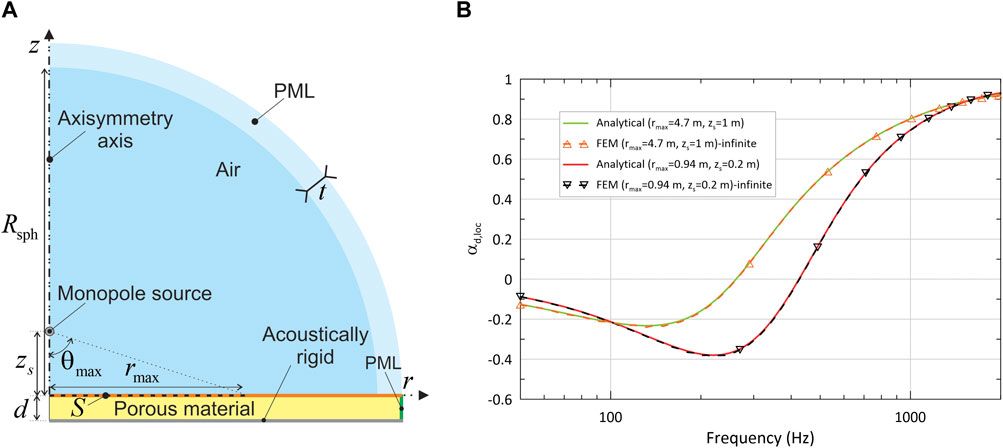
The calculation of the SAC ${\alpha }_{\mathrm{d},\text{loc}}$ (Eq. 10) based on the local reflection coefficient obtained with Eq. 3 and 4 is verified through comparison with a FE model solved in COMSOL Multiphysics 6.2. This FE model has been validated by comparing the simulated and measured transfer function between two microphones above a finite extent melamine sample for two different source positions (Berry, 2024; Sciard et al., 2024) and therefore serves as a reference. To replicate the configuration of the analytical model—consisting of a rigid-backed laterally infinite material coupled to a semi-infinite air domain—the FE model incorporates a cylinder with a sufficiently large radius ${\mathit{R}}_{\text{sph}}$ and thickness d backed by a rigid wall. The porous material interfaces with a hemispherical air domain of radius $R_{\text{sph}}$. A perfectly matched layer (PML) ring of thickness $t$ is placed around the air sphere to simulate the Sommerfeld condition. Along the lateral boundary of the porous material, another PML is applied to absorb waves radially, simulating the material’s infinite nature in this direction. The monopole source is assumed to be positioned on the cylinder axis at height $z_s$ above the material. Given the axisymmetric nature of the problem, a 2D-axisymmetric model is solved (see Figure 2A for a cross-section in the $\left(r,z\right)$ plane). In Figure 2A, the orange line denotes the interface between the porous material and the air, while the vertical green edge corresponds to the PML boundary condition for the porous material. The SAC ${\alpha }_{\mathrm{d},\text{loc}}$ defined by Eq. 10 is computed using both the analytical and the FE models on a disk of radius $r_{\max }$ (surface S delineated by a dashed black line). In the FE model, the local reflection coefficient ${\widehat{R}}_{loc}\left(r,z_s,\omega \right)$ is calculated from the reflected sound pressure obtained by making the difference between the total sound pressure above the material resulting the FE solving and the incident sound pressure given by Eq. 3.

Figure 2

Figure 2. (A) 2D-axisymmetric finite element model of an infinite lateral extent porous material used for verification (cross-section in the $\left(r,z\right)$ plane) [Adapted with permission from (Sgard et al., 2024). Copyright 2024, Acoustical Society of America.] (B) Sound absorption coefficient ${\alpha }_{\mathrm{d},\text{loc}}$ of a melamine foam ($d=$ 5 cm) for ${\theta }_{\max }$ = 78°–comparison between the present analytical approach (Analytical) and FE simulation (FEM) for two source heights $z_s$ = 0.2 m and $z_s$ = 1 m.

In the ensuing analysis, computations are conducted within the frequency range of 50–2000 Hz for a 5 cm-thick melamine material, with a ${\theta }_{\max }$ value of 78° examined at two different source heights ($z_s$ = 0.2 m and 1 m). This corresponds to two distinct radii: $r_{\max }$ = 0.94 m and 4.7 m. The FE model used values of $R_{\text{sph}}$ = 8 m and $t$ = 8 cm. The JCA parameters in Table 1 are used for the analytical approach and the FE model. The FE meshes allow for convergence of the SAC ${\alpha }_{\mathrm{d},\text{loc}}$ calculations up to 2000 Hz.

Figure 2B plots ${\alpha }_{\mathrm{d},\text{loc}}$ between 50 Hz and 2000 Hz with a frequency step of 10 Hz. Excellent agreement between the analytical model and the FE model is obtained for both source positions, verifying the analytical model for calculating ${\alpha }_{\mathrm{d},\text{loc}}$.

3.2 Finite size effect and boundary conditions of the porous material

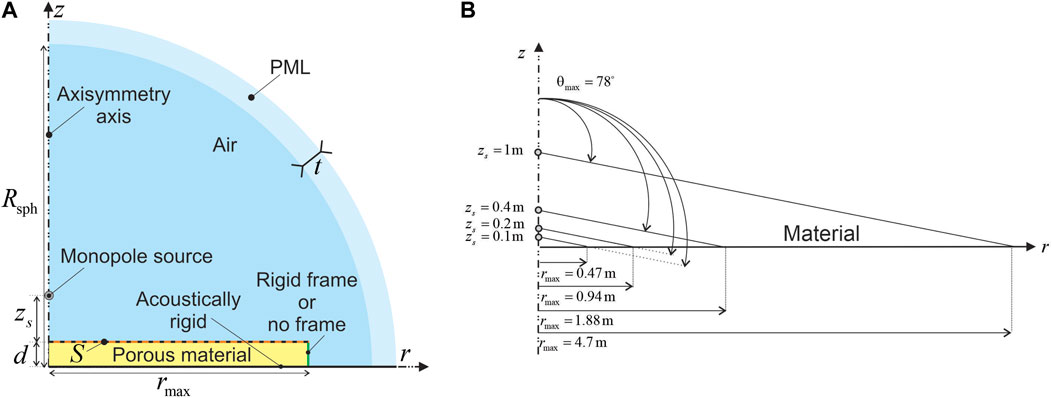
In practice, the porous sample is of finite size. However when calculating ${\alpha }_{\mathrm{d},\text{loc}}$ (Eq. 10) using the analytical model based on Eqs 3 and 4, the reflected sound pressure field utilized in Eq. 4 is the one above a material with infinite lateral extent. Thus, the analytical model does not account for the scattering due to the finite size, nor considers the boundary condition on the lateral side of the sample. If the analytical model is to be used to estimate ${\alpha }_{\mathrm{d},\text{loc}}$ of a sample of radius $r_{\max }$, the error committed by neglecting the aforementioned effects must be evaluated. This is achieved by comparing the SAC obtained through the analytical model with that obtained through a FE model of a material sample of finite size and given boundary conditions. Thus, the FE model configuration comprises a porous material cylinder of radius $r_{\max }$ and thickness $d$, situated within a semi-anechoic room and resting on a rigid floor (Figure 3A).

Figure 3

Figure 3. (A) 2D-axisymmetric FE model of a finite size rigid-backed porous material (cross-section in the $\left(r,z\right)$ plane) [Adapted with permission from (Sgard et al., 2024). Copyright 2024, Acoustical Society of America.] (B) Source positions and material lateral extents $r_{\max }$ of interest corresponding to ${\theta }_{\max }={78}^{\circ }$

The finite element (FE) model resembles that depicted in Figure 2A. The porous material is coupled with a hemispherical air domain of radius $R_{\text{sph}}$ surrounded by a PML of thickness $t$. This configuration is devised to emulate a semi-infinite air domain. In Figure 3A, the interface between the porous material and the air domain is delineated by the black–orange dashed line. The green line indicates the lateral boundary of the porous material. Two distinct boundary conditions are applied to this vertical edge: a rigid-wall boundary condition, termed the “rigid frame”, and a coupling condition, labeled the “no frame”. The former involves surrounding the material with a rigid frame (null normal particle velocity) while the latter establishes a coupling between the porous material and the surrounding air, ensuring continuity of sound pressure and normal particle velocity. Subsequently, ${\widehat{\mathfrak{R}}}_{\text{loc}}\left(r,z_s,\omega \right)$ is computed for both the analytical and FE models and substituted in Eq. 10 to obtain ${\alpha }_{\mathrm{d},\text{loc}}$. Similarly to section 3.1, in the FE model, the local reflection coefficient ${\widehat{R}}_{loc}\left(r,z_s,\omega \right)$ is calculated from the reflected sound pressure obtained by making the difference between the total sound pressure above the material resulting the FE solving and the incident sound pressure given by Eq. 3. For the FE model, values $t$ = 8 cm and $R_{\text{sph}}=r_{\max }+0.5$m are used, and the meshes allow for convergence of ${\alpha }_{\mathrm{d},\text{loc}}$ in the frequency band of interest (50-4,000 Hz).

Computations have been conducted for a melamine foam specimen (see Table 1 for parameters). Figure 4 displays a comparative analysis between the analytical model and FE simulations under “rigid frame” and “no frame” boundary conditions for various radii $r_{\max }$ and source heights, considering two material thicknesses of 5 cm and 20 cm. Notably, the thickness of the material may exert a discernible influence on the manifestation of boundary effects. Angle ${\theta }_{\max }$, corresponding to the solid angle that the material subtends from the source position, has been fixed at ${78}^{\circ }$, which corresponds to field incidence. Source heights of $z_s=$ 0.1 m, 0.2 m, 0.4 m, and 1 m have been considered. The sample radii $r_{\max }=$ 0.47 m, 0.94 m, 1.88 m, and 4.7 m were selected accordingly using $r_{\max }=z_s\tan {\theta }_{\max }$ (Figure 3B).

Figure 4

Figure 4. ${\alpha }_{\mathrm{d},\text{loc}}$ as a function of frequency for 5 cm thick and 20 cm thick melamine for various source heights and values of $r_{\max }$ for ${\theta }_{\max }={78}^{\circ }$ (see Figure 3B). Comparison between the present approach (analytical) and FE simulation accounting for two different material lateral boundary conditions (rigid frame and no frame) for (A) $r_{\max }=$ 0.47 m, $z_s=$ 0.1 m (B) $r_{\max }=$ 0.94 m, $z_s=$ 0.2 m (C) $r_{\max }=$ 1.88 m, $z_s=$ 0.4 m, and (D) $r_{\max }=$ 4.7 m, $z_s=$ 1 m.

Figure 4 shows that for the material sizes and the two thicknesses considered here, there is no difference between the “rigid frame” and “no frame” boundary conditions for ${\alpha }_{\mathrm{d},\text{loc}}$ computed with the FE approach. Above 600 Hz, both analytical and FE models yield the same results. Consequently, in this frequency range the material finite size has no effect on ${\alpha }_{\mathrm{d},\text{loc}}$. Discrepancies between the analytical and FE models arise at low frequencies (<600 Hz for $r_{\max }=$0.47 m, <400 Hz for $r_{\max }=$ 0.94 m, <300 Hz for $r_{\max }=$ 1.88 m, and <200 Hz for $r_{\max }=$ 4.7 m). As expected, the impact of the finite size is more pronounced as $r_{\max }$ (size) decreases and $d$ (thickness) increases. For $r_{\max }\ge 1.88$m (Figures 4C, D), the deviations stay minor (maximum values <0.04 for $d$ = 5 cm and <0.08 for $d$ = 20 cm) below 150 Hz. For $r_{\max }=$ 0.94 m (Figure 4B), the discrepancies remain minimal and occur below 400 Hz (maximum values <0.08 for $d$ = 5 cm and <0.11 for $d$ = 20 cm). For $r_{\max }=$ 0.47 m (Figure 4A), the magnitude of deviations slightly increases with maximum values of 0.14 for $d$ = 5 cm and 0.15 for $d$ = 20 cm below 210 Hz. Consequently, if one’s focus lies on scenarios involving materials whose characteristics align with what is studied in this paper, assuming a minimum sample dimension $r_{\max }$ greater than about 1 m ensures that the boundary effects of the material are of minor importance, and employing the analytical model yields accurate approximations of ${\alpha }_{\mathrm{d},\text{loc}}$ across materials with finite size of radius $r_{\max }$. To accurately assess the acoustic absorption behavior of the material samples when their radial extents fall below 1 m and frequencies are below 600 Hz, it is necessary to incorporate considerations for both finite size and boundary conditions, such as utilizing a Finite Element (FE) modeling approach. It must be noted that the identified limit of 1 m relies upon specific material properties, thicknesses, and source heights explored in this study, which could vary depending on configurations diverging from those presented herein. Therefore, caution should be exercised when extrapolating these findings outside the scope of the current investigation. Subsequently, only material samples with radius $r_{\max }$ larger than 1 m will be considered and the analytical model will be employed to calculate the associated ${\alpha }_{\mathrm{d},\text{loc}}$.

3.3 Use of ${\mathit{\alpha }}_{\mathrm{d},\text{loc}}$ to approximate ${\mathit{\alpha }}_{\mathrm{d}}$

The goal of this section is now to assess the limits of using the diffuse field SAC ${\alpha }_{\mathrm{d},\text{loc}}$ (Eq. 10) obtained from the oblique incidence local reflection coefficient under a monopole excitation for various receiver locations on the material surface to approximate the classical diffuse field SAC ${\alpha }_{\mathrm{d}}$ (Eq. 9) calculated from plane wave reflection coefficient. It should be recalled that for values of $r_{\max }$ larger than about 1 m, the analytical model based on Eq. 10 for calculating ${\alpha }_{\mathrm{d},\text{loc}}$ provides a very good approximation to results obtained for finite-size materials of radius $r_{\max }$.

Figures 5 and 6 display the corresponding SACs of a melamine foam (see Table 1) for thicknesses of 0.01 m, 0.05 m, and 0.2 m as a function of frequency for three source heights (20 m, 2 m, and 0.2 m) and two values of limit angle ${\theta }_{\max }$, respectively. Recall that ${\theta }_{\max }$ corresponds to the maximum angle of incidence that could be achieved when measuring the local reflection coefficient using, for example, a microphone doublet. This angle is obtained when the microphone doublet is located at the outer boundary of the material. The corresponding radial distance is thus equal to $r_{\max }$. Since the limit angles and the monopole heights are fixed, values of $r_{\max }$ corresponding to ${\theta }_{\max }$ are determined using $r_{\max }=z_s\tan {\theta }_{\max }$ in the calculation of ${\alpha }_{\mathrm{d},\text{loc}}$. In the following, ${\theta }_{\max }$ is equal either to ${90}^{\circ }$ or ${78}^{\circ }$. ${\theta }_{\max }={90}^{\circ }$ corresponds to an infinite lateral extent material. In order to obtain the SAC of a laterally infinite material, the value of $r_{\max }$ is increased progressively by doubling its value at each step, starting from $r_{\max }=$ 1 m until the metric $\varpi ={\displaystyle \sum _f}\Delta {\alpha }_{\mathrm{d},\text{loc}}\left(f\right)/{\displaystyle \sum _f}{\alpha }_{\mathrm{d},\text{loc}}^{\left(N\right)}\left(f\right)$ is below 0.005 in the frequency range of computation (50–4,000 Hz). In the previous metric, the sum ${\displaystyle \sum _f}$ is carried out over discrete frequencies in the interval 50–4,000 Hz (frequency step of 10 Hz). In addition, $\Delta {\alpha }_{\mathrm{d},\text{loc}}$ represents the absolute value of the difference between the value of ${\alpha }_{\mathrm{d},\text{loc}}$ calculated at steps N and N-1—that is, for $r_{\max }=r_{\max }^{\left(N-1\right)}=2^{N-1}$ m and for $r_{\max }=r_{\max }^{\left(N\right)}=2^N$ m. Sufficiently large values of $r_{\max }$ are thus chosen for ${\alpha }_{\mathrm{d},\text{loc}}$ to converge towards ${\alpha }_{\mathrm{d},\text{loc},\infty }$ according to the criterion $\varpi \le 0.005$. ${\theta }_{\max }={78}^{\circ }$ corresponds to the common value used for field incidence. In this case, the radial distances $r_{\max }$ associated with the three source heights are indicated in the legends of Figures 6A–C.

Figure 5

Figure 5. Comparison of two ways (Eqs 9, 10) of calculating the sound absorption coefficients for three source heights 20 m, 2 m, and 0.2 m as a function of frequency for ${\theta }_{\max }={90}^{\circ }$ and a melamine of thickness $d$ (A) 1 cm (B) 5 cm (C) 20 cm.

Figure 6

Figure 6. Comparison of two ways (Eqs 9, 10) of calculating the sound absorption coefficients for the source heights 20 m, 2 m, and 0.2 m as a function of frequency for ${\theta }_{\max }={78}^{\circ }$ and a melamine of thickness $d$ (A) 1 cm (B) 5 cm (C) 20 cm.

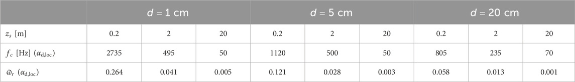
To quantify the global error over the whole frequency range of interest between ${\alpha }_{\mathrm{d},\text{loc}}$ and ${\alpha }_{\mathrm{d}}$, a relative error defined as ${\varpi }_r={\displaystyle \sum _f}\left|{\mathrm{\alpha }}_{d,loc}\left(f\right)-{\alpha }_d\left(f\right)\right|/{\displaystyle \sum _f}{\alpha }_d\left(f\right)$ is introduced. One also considers a frequency referred to as $f_c$ above which the absolute error between ${\mathrm{\alpha }}_{d,loc}\left(f\right)$ and ${\alpha }_d\left(f\right)$ is less than a given threshold $ϵ$. The approximation is considered good when $ϵ$ = 5%. Tables 2 and 3 display the values of ${\varpi }_r$ and $f_c$ for the considered configurations when ${\theta }_{\max }={90}^{\circ }$ and ${78}^{\circ }$, respectively.

Table 2

Table 2. Values of frequency $f_c$ for ${\alpha }_{\mathrm{d},\text{loc}}$ and values of error ${\text{ϖ}}_r$ between ${\alpha }_{\mathrm{d},\text{loc}}$ and the reference ${\alpha }_{\mathrm{d}}$ in each configuration for ${\theta }_{\max }={90}^{\circ }$

Table 3

Table 3. Values of frequency $f_c$ for ${\alpha }_{\mathrm{d},\text{loc}}$ and values of the error ${\text{ϖ}}_r$ between ${\alpha }_{\mathrm{d},\text{loc}}$ and the reference ${\alpha }_{\mathrm{d}}$ in each configuration for ${\theta }_{\max }={78}^{\circ }$

3.3.1 Case ${\mathit{\theta }}_{\max }={\mathrm{90}}^{\circ }$

Table 2 and Figure 5 show that for a given thickness, $f_c$ decreases with the source height. ${\alpha }_{\mathrm{d},\text{loc}}$ is a good approximation of ${\alpha }_{\mathrm{d}}$ at mid to high frequencies for $z_s=$ 2 m and $z_s=$ 0.2 m and at all frequencies for $z_s=$ 20 m (source in the far field). Below $f_c$, ${\alpha }_{\mathrm{d},\text{loc}}$ is always smaller than ${\alpha }_{\mathrm{d}}$ and can even be negative. This potential for negative values arises from the approximation inherent in Eq. 8, which assumes that the incident and reflected sound pressure field wavefronts are planar—a condition that does not hold true at low frequencies as mentioned in Sections 2.2.2 and 2.2.3. In general, when thickness $d$ of the material increases for a given source height ($z_s=$ 0.2 m and $z_s=$ 2 m), the frequency $f_c$ beyond which a good approximation holds is shifted to lower frequencies (Table 2). One exception is observed when the thickness is changed from 1 cm to 5 cm for $z_s=$ 20 m where frequency $f_c$ rather increases but the difference between the two frequencies is very small and is close to the lower limit of the frequency band of interest. The approximation deteriorates at low frequencies when the source gets closer to the material and the material gets thinner. Overall, as seen in Table 2, global error ${\varpi }_r$ decreases with the material thickness for a given source height and with the source height for a given thickness.

3.3.2 Case ${\mathit{\theta }}_{\max }={\mathrm{78}}^{\circ }$

When ${\theta }_{\max }$ is reduced to ${78}^{\circ }$, increasingly smaller material surfaces are involved as $z_s$ decreases (Figure 3B). Overall, Table 3 shows that the global error ${\varpi }_r$ for a given configuration is reduced when compared to ${\theta }_{\max }={90}^{\circ }$. The same trends as Table 2 are observed regarding the error decrease with the material thickness for a given source height and with the source height for a given thickness. Figure 6 indicates that similar observations as for ${\theta }_{\max }={90}^{\circ }$ can be made in the case ${\theta }_{\max }={78}^{\circ }$.

4 Conclusion

This study numerically investigated the error between the diffuse field SAC ${\alpha }_{\mathrm{d}}$ of a porous material, calculated from plane wave reflection coefficients and that obtained from local oblique incidence reflection coefficients for a monopole excitation, referred to as ${\alpha }_{\mathrm{d},\text{loc}}$. The local reflection coefficient has been analytically determined using Allard’s model, which describes sound propagation above a porous material of infinite lateral extent backed by a rigid wall and excited by a monopole. Comparisons have been made between ${\alpha }_{\mathrm{d},\text{loc}}$ and ${\alpha }_{\mathrm{d}}$ for a melamine foam sample as functions of material extent, thickness, and source height for two limit angles.

The key findings are:

• The analytical model provides a good approximation of the local SAC ${\alpha }_{\mathrm{d},\text{loc}}$ for finite-size materials, with a radius exceeding 1 m for the configurations studied. However, the threshold value may vary for other configurations (material properties, thickness, source height). In general, for materials of finite lateral extent, a more sophisticated model (e.g., FE) can be used to predict ${\alpha }_{\mathrm{d},\text{loc}}$ very accurately. The analytical model enables calculation of SAC ${\alpha }_{\mathrm{d},\text{loc}}$ for an infinite material, using substantial values of radius $r_{\max }$.

• ${\alpha }_{\mathrm{d},\text{loc}}$ was found to be a good approximation of the diffuse field SAC ${\alpha }_{\mathrm{d}}$ for random and field incidences at mid to high frequencies, but its accuracy decreases at low frequencies, especially when the source is close to the material and the material is thin.

• Increasing the monopole height improves accuracy at lower frequencies, provided that the material area is chosen appropriately relative to the source height to ensure the proper limit angle.

• For material surfaces typically encountered in laboratory conditions and when the source is close to the material, one can expect to approximate the field incidence diffuse field ${\alpha }_{\mathrm{d}}$ using ${\alpha }_{\mathrm{d},\text{loc}}$ only at mid to high frequencies and for sufficiently thick materials.

Additional simulations for other homogenous porous materials (felt, fibers, and foams similar to those considered in Sgard et al. (2024)) were conducted using the analytical model within its domain of validity. Although not reproduced here for sack of concision, these simulations showed similar trends in the application of ${\mathrm{\alpha }}_{\mathrm{d},\text{loc}}$ as an approximation of ${\mathrm{\alpha }}_{\mathrm{d}}$. Further work would involve an experiment to corroborate the numerical observations.

Data availability statement

The raw data supporting the conclusion of this article will be made available by the authors without undue reservation.

Author contributions

FS: Conceptualization, Formal Analysis, Funding acquisition, Investigation, Methodology, Software, Validation, Visualization, Writing–original draft, Writing–review and editing. NA: Conceptualization, Methodology, Software, Validation, Writing–review and editing. OR: Writing–review and editing.

Funding

The authors declare that financial support was received for the research, authorship, and/or publication of this article. This research has been funded by IRSST (grant 2018-0027).

Acknowledgments

The authors acknowledge the support of the IRSST for funding this research. This paper benefited from the application of OpenAI’s GPT-3, version 3.5, generative AI technology, which was employed to enhance the linguistic accuracy and quality of the content.

Conflict of interest

The authors declare that the research was conducted in the absence of any commercial or financial relationships that could be construed as a potential conflict of interest.

Publisher’s note

All claims expressed in this article are solely those of the authors and do not necessarily represent those of their affiliated organizations, or those of the publisher, the editors and the reviewers. Any product that may be evaluated in this article, or claim that may be made by its manufacturer, is not guaranteed or endorsed by the publisher.

References

Allard, J.-F., and Atalla, N. (2009). Propagation of sound in porous media: modelling sound absorbing materials. 2nd edn. Wiley-Blackwell.

Google Scholar

Allard, J.-F., Lauriks, W., and Verhaegen, C. (1992). The acoustic sound field above a porous layer and the estimation of the acoustic surface impedance from free-field measurements. J. Acoust. Soc. Am. 91 (5), 3057–3060. doi:10.1121/1.402941

CrossRef Full Text | Google Scholar

Berry, A. (2024). Development of a measurement system for the characterization of absorbent treatments in the laboratory by optimization of an innovative method and creation of a database of absorption coefficients (in french ‘Développement d’un système de mesure pour la caractérisation des traitements absorbants en laboratoire - Optimisation d’une méthode innovante et création d’une base de données de coefficients d’absorption’). Research Report R-1186-fr. Montréal, QC, Canada: IRSST, 131.

Google Scholar

Bies, D. A., and Hansen, C. H. (2014). “Engineering noise control: theory and practice,”. 3rd edn. London: CRC Press. doi:10.1201/9781482264739

CrossRef Full Text | Google Scholar

Dragonetti, R., Opdam, R., Napolitano, M., Romano, R., and Vorländer, M. (2016). Effects of the wave front on the acoustic reflection coefficient. Acta Acustica united Acustica 102 (4), 675–687. doi:10.3813/AAA.918984

CrossRef Full Text | Google Scholar

Dragonetti, R., and Romano, R. A. (2015). Considerations on the sound absorption of non locally reacting porous layers. Appl. Acoust. 87, 46–56. doi:10.1016/j.apacoust.2014.06.011

CrossRef Full Text | Google Scholar

Hopkins, C. (2007). Sound insulation. 1st edn. Amsterdam: Elsevier/Butterworth-Heinemann.

Google Scholar

Kuipers, E. R., Wijnant, Y. H., and De Boer, A. (2012). A numerical study of a method for measuring the effective in situ sound absorption coefficient. J. Acoust. Soc. Am. 132 (3), EL236–EL242. doi:10.1121/1.4745839

PubMed Abstract | CrossRef Full Text | Google Scholar

Kuipers, E. R., Wijnant, Y. H., and De Boer, A. (2014). Measuring sound absorption: considerations on the measurement of the active acoustic power. Acta Acustica united Acustica 100 (2), 193–204. doi:10.3813/AAA.918699

CrossRef Full Text | Google Scholar

Nobile, M. A. (2005). The spherical wave absorption coefficient of a patch of material. J. Acoust. Soc. Am. 85 (S1), S61. doi:10.1121/1.2027070

CrossRef Full Text | Google Scholar

Paris, E. T. (1928). L.On the coefficient of sound-absorption measured by the reverberation method. Lond. Edinb. Dublin Philosophical Mag. J. Sci. 5 (29), 489–497. doi:10.1080/14786440308565092

CrossRef Full Text | Google Scholar

Pierce, A. D. (1989). Acoustics, an introduction to its physical principles and applications. New York, USA: McGraw-Hill.

Google Scholar

Robin, O., Berry, A., Doutres, O., and Atalla, N. (2014). Measurement of the absorption coefficient of sound absorbing materials under a synthesized diffuse acoustic field. J. Acoust. Soc. Am. 136, EL13–19. doi:10.1121/1.4881321

PubMed Abstract | CrossRef Full Text | Google Scholar

Robin, O., Berry, A., Kafui Amédin, C., Atalla, N., Doutres, O., and Sgard, F. (2019). Laboratory and in situ sound absorption measurement under a synthetized diffuse acoustic field. Build. Acoust. 26 (4), 223–242. doi:10.1177/1351010X19870307

CrossRef Full Text | Google Scholar

Sciard, M., Berry, A., Sgard, F., Dupont, T., and Robin, O. (2024). Estimation of acoustical materials sound absorption coefficient under oblique incidence plane wave and diffuse field via Allard model inversion. Build. Acoust. 31, 147–175. doi:10.1177/1351010X241235515

CrossRef Full Text | Google Scholar

Sgard, F., Atalla, N., Robin, O., and Berry, A. (2024). On the area-averaged effective sound absorption coefficient of porous materials excited by a monopole. J. Acoust. Soc. Am. 155 (2), 1135–1150. doi:10.1121/10.0024767

PubMed Abstract | CrossRef Full Text | Google Scholar

Shampine, L. F. (2008). Vectorized adaptive quadrature in MATLAB. J. Comput. Appl. Math. 211 (2), 131–140. doi:10.1016/j.cam.2006.11.021

CrossRef Full Text | Google Scholar

Thomasson, S. (1977). Sound propagation above a layer with a large refraction index. J. Acoust. Soc. Am. 61 (3), 659–674. doi:10.1121/1.381352

CrossRef Full Text | Google Scholar