Space-time reconstruction of a moving acoustic loading on a membrane by coupling the force analysis technique and full-field non-contact vibration measurements

Identifying acoustical and mechanical loadings on structures is a common problem in acoustics and vibration analysis and stationary loadings are mostly considered on plate-like structures. This work describes a proof of concept for reconstructing the trajectory of an acoustic source moving in front of a membrane. Compared with works focusing on precisely identifying a loading’s amplitude at a given location, the objective is to reconstruct the loading’s trajectory–Qualitative loading identification is sought rather than quantitative. The force analysis technique is used to recover a space-time varying loading on a structure, starting from time-resolved full-field non-contact vibration measurements conducted on a circular membrane. At the same time, a compact and tonal sound source is used to draw freehand shapes in front of the membrane. The loading trajectory, therefore, contains information that was “acoustically written”. Simple hand gestures that correspond to the drawing of a Greek letter (Σ), a capital letter (P), two shapes (♡, ⋆), and a 3-letter word (net) are recovered using the proposed procedure. The effect of various parameters on the reconstructed information is studied. Perspectives in terms of possible research areas and applications are finally discussed. These perspectives include, for example, the use of membranes to help reconstruct complex and space-time-varying loadings or even applications in musical acoustics on membranophones.

1 Introduction

Force or loading identification techniques in structures are commonly used to solve engineering-based problems, usually called inverse problems. Indeed, these techniques aim to recover the input into a system knowing its output, that is, the system’s response. In the review article by (Sanchez and Benaroya, 2014), identification techniques are divided into three families: (1) methods that make direct use of a physical or mathematical model to formulate the inverse problem, (2) regularization methods to reduce the ill-posedness nature of the problem, and (3) statistical and probabilistic methods. It is beyond the scope of this paper to summarize and describe all these techniques, and the interested reader can consult Reference (Sanchez and Benaroya, 2014) and bibliographical references 1–30 in (Logan et al., 2020). The identification method considered in this work, the force analysis technique, falls into the first category of the three identification families proposed in (Sanchez and Benaroya, 2014). The force analysis technique was developed by (Pézerat and Guyader, 1995; Pézerat and Guyader, 2000) and directly uses the equation of motion of a structure to solve the inverse problem. In practical terms, vibration measurements made on a system are used to identify the loading that puts the system in vibration. This technique was initially developed for beams and thin plates (Pézerat and Guyader, 2000) and was also applied to shells (Djamaa et al., 2007) and finite element models (Renzi et al., 2013). Applications range from localization and magnitude estimation of mechanical loading to identification of distributed pressure loading like an acoustic plane wave, a diffuse acoustic field (Leclere and Pézerat, 2008), or a turbulent boundary layer (Lecoq et al., 2014). In addition to loading identification problems, the force analysis technique was extended to identify mechanical parameters such as Young’s modulus or the structural loss factor (Ablitzer et al., 2014). Another use of this technique was suggested by (Leclère and Picard, 2015). In their work, a loudspeaker to be localized was placed in a semi-anechoic room, this room being coupled to a reverberant room. An aluminum panel was positioned in the wall, separating the two chambers. Measuring the panel’s vibration field using a scanning laser vibrometer (reverberant room side) allowed the identification of the incident sound pressure field (semi-anechoic room side). This field was then used as an input for an acoustic source localization method (beamforming), and the physical position of the source in the semi-anechoic room was finally retrieved. Although this work was limited to stationary excitations, given the scanning operation of the laser, extended information was obtained compared with the classical use of identification techniques. Not only was the loading identified, but the information it conveyed was used to extract additional features to feed additional post-processing routines - here, by finally localizing a sound source through a rigid separation between two rooms.

Acoustic source localization plays a crucial role in acoustics, and a first example lies in applications related to non-destructive testing and structural health monitoring, that is when acoustic emission from a structural failure must be identified and localized (Yin et al., 2019). To achieve localization, a cluster of ultrasonic sensors is usually placed on a structure to collect information from the propagation of elastic waves. Acoustic source localization can also extend to acoustic touchscreen technologies (Phares, 2016). Touch detection and tracking approaches use various arrangements of emitters, receivers, and algorithms, including the acoustic pulse recognition (Reis et al., 2010), the surface acoustic wave (Drafts, 2001), and time reversal (Kent, 2010). Industry, transportation, and building are domains for which acoustic source localization has become an active research area in recent years, given the technical advances in data acquisition and processing. In that case, a microphone array is typically used to identify and localize sound sources to propose noise reduction approaches or to gain an improved knowledge of a given acoustics-related problem. Standard methods aim to process signals from an array of sensors, including beamforming (Chiariotti et al., 2019) and generalized cross-correlation (Knapp and Carter, 1976; Quaegebeur et al., 2016). In those works, the sound sources that must be localized and possibly quantified are generally stationary and at a fixed location. Indeed, characterizing moving sources is more challenging than stationary sources due to the time-varying spatial location and possible frequency shifts at the receiver’s position caused by the non-stationary motion and Doppler effect (Meng et al., 2019; Chen and Lu, 2020).

In this work, another kind of acoustic source localization is sought. The force analysis technique is indeed used to recover a space-time-varying loading on a membrane, starting from time-resolved full-field and non-contact vibration measurements conducted on this structure. The loading is created by a person pointing at the membrane with a handheld acoustic source and using this acoustic source to draw letters, symbols, or words. The emitter is a person “acoustically drawing,” the receiver is a camera, and the modem is a vibrating membrane. Our goal is to investigate the possibility of reconstructing the trajectory of that mobile sound source.

The first originality of this work is the application of the force analysis technique on a membrane, which has not yet been reported to the best of our knowledge (only the reconstruction of the magnitude of a turbulent boundary layer loading using the virtual field method and a membrane was considered in (O’Donoughue et al., 2019b)). This is most likely because vibration measurements on such light structures using contact sensors would be largely biased and complex to set up. The use of non-contact and full-field vibration measurements opens up this specific perspective. This work’s second originality consists of combining the force analysis technique with full-field and non-contact vibration measurements (here, deflectometry), allowing a sound pressure loading identification as a function of time and space. Most of the research that used the force analysis technique was conducted in the frequency domain, restricted to stationary and mechanical excitations, and used arrays of physical sensors like accelerometers. The virtual field method was also combined with deflectometry in (Kaufmann et al., 2019) to reconstruct the pressure distribution on a plate due to a fixed air jet, an aerodynamic load of several hundred of Pascal magnitude. In the present case, the loading is mobile, and the sound pressure amplitude is in the order of 1 Pa.

The paper is organized as follows. The Method section introduces the deflectometry technique, recalls the theory elements concerning the equation of motion and the force analysis technique for a membrane, and details the experimental setup and test conditions. The Results section presents the results obtained, including the analysis of the effect of several influential parameters. The Discussion section starts with a possible application of the proposed work. We also detail the potential and limitations of this proof-of-concept and suggest future works to improve the quality of trajectory reconstruction and take into account more parameters, such as the source’s frequency and its travelling speed. This last section also concludes the paper by summarizing the main results and suggesting three perspectives for combining the force analysis technique with full-field non-contact vibration measurements on a membrane.

2 Methods

2.1 Deflectometry technique

Deflectometry is an optical technique that directly provides a full-field measurement of local slopes (α_x,y, first-order derivatives of the surface shape), estimated from an image that is observed by specular reflection on a flat structure (Devivier et al., 2012; O’Donoughue et al., 2021). This latter must have a mirror-like finish to satisfy the specular reflection condition. Deflectometry is widely used to assess the condition of reflective surfaces (Burke et al., 2023). The image observed on the reflective surface is the reflection of a 2D grid, and is sensitive to plane changes: an imperfection in the shape of the surface leads to conspicuous distortions in the virtual image. Similarly, the deflectometry technique is sensitive to small out-of-plane surface deformations and is, therefore, well suited to measuring the dynamic bending of thin, flat structures. A typical measurement configuration is illustrated in Figure 1A. The observed image is a regular 2D grid placed at a distance L from the reflective surface under study. Any transverse loads applied to the structure will distort the grid image seen by the camera. Surface slope variation in the x and y directions are directly proportional to the local phase variations Φ of the grid lines in the images. Phase variations for the structure under excitation are obtained by comparing phase mappings calculated from the reference image (undeformed grid image) and a distorted image (deformed grid image).

FIGURE 1

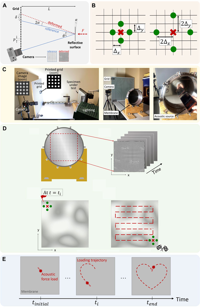
FIGURE 1. (A) Scheme of deflectometry measurement on a plane structure. (B) A 5-point centered finite difference scheme for estimating second-order spatial derivative terms (over a regular Cartesian grid). (C) Left - Side view: General experimental setup for deflectometry measurements (based on data from O’Donoughue, 2020); Middle - Global view: Experimental setup for measurement on a membrane; Right - Close-up view: experimental setup for measurement on a membrane with a smartphone as the acoustic source. (D) Explanatory scheme of the followed procedure, from left to right and from top to bottom Pictures of the reflected grid are taken on a square over the membrane; The slopes and then displacement maps are calculated on a regular grid as a function of t_i; For each time step, the 5-point finite difference scheme starts from an initial position; The 5-point scheme scans the whole membrane. (E) Scheme of the trajectory followed by the acoustic source along the membrane surface during measurement (heart shape test case).

For a local phase variation Φ at a given point on the structure, the observed point in the grid is translated by a distance $\delta =\frac{p}{2\pi }\mathrm{\Phi }$ where p is the pitch of the grid (spatial grid period) (O’Donoughue et al., 2023). In the small angle approximation for θ and α, this distance is equivalent to δ = 2Lα. Combining the two formulas for δ allows deducing the slope fields on the surface structure from the resulting phase maps Φ_x,y using the following geometrical relation:

${\alpha }_{x,y}=\frac{p}{4\pi L}{\mathrm{\Phi }}_{x,y}.(1)$

Transversal displacements can be then obtained by performing an inverse gradient on the slope (a spatial integration since ${\alpha }_i(x,y)=\frac{\partial w}{\partial i}(x,y)$, with i = x, y). It is underlined that in the presented deflectometry measurements and other works (O’Donoughue et al., 2019a), local spatial phase variations Φ are evaluated using a phase-stepping approach with a windowed discrete Fourier transform (WDFT) algorithm (Sur and Grédiac, 2016). Other approaches could be used. For example, deflectometry measurements were coupled with a particle image velocimetry tool in (O’Donoughue et al., 2021) and were adequately post-processed with that tool compared to the WDFT algorithm.

2.2 Equation of motion and force analysis technique for a membrane

Plates were primarily considered in works related to the force analysis technique. In that case, the equation of motion includes fourth-order derivatives along x and y directions and second-order cross-derivative, and a 13-point finite difference scheme is used to evaluate those derivatives (Pézerat and Guyader, 1995; 2000; Leclere and Pézerat, 2008; Ablitzer et al., 2014; Lecoq et al., 2014; Leclère et al., 2015). Using a finite difference scheme introduces an approximation that can amplify measurement noise or uncertainties, especially with increasing order derivations. Several approaches were proposed to limit those issues, such as low-pass wave number filtering (Pézerat and Guyader, 2000), adapted separation for the sensors (Leclère et al., 2014), or a more elaborate correction for the bias induced by the finite difference scheme, called the corrected force analysis technique (Leclère et al., 2015). In the case of a membrane, only second-order derivatives are involved, limiting these undesirable side effects compared with the plate case. Therefore, no specific post-processing was applied to the measured data. The equation of motion for a membrane subjected to a given excitation F writes

$T\left(1+\mathrm{j}\eta \right)\left(\frac{{\partial }^{2}w}{\partial x^2}+\frac{{\partial }^{2}w}{\partial y^2}\right)-\rho h\frac{{\partial }^{2}w}{\partial t^2}=-F\left(x,y,t\right),(2)$

where w is the normal displacement of the membrane, T its static tension, j the imaginary number, η the structural loss factor of the membrane, ρ its mass density, and h its thickness.

By knowing the membrane’s mechanical parameters and having access to its displacement field, the time and space distribution of the force can be estimated. More precisely, the goal of the force analysis technique is to directly calculate the left-hand side of Eq. 2 to evaluate its right-hand side, the force distribution F (x, y, t). Note that no specific knowledge of the boundary conditions or excitation is required (that is, the boundary conditions or excitations that lay outside the local region where the equation is solved). Indeed, the equation of motion is locally solved, so knowing the displacement field on the whole structure is not required, but only on the subsection of the structure where the force distribution is to be identified (Pézerat and Guyader, 1995; 2000).

The spatial derivatives of Eq. 2 are approximated using a second-order finite difference scheme (backward and forward at the limits of the structure and centered otherwise). Arrays of accelerometers have been mainly used to implement the finite difference scheme and calculate the second term on the left-hand side of Eq. 2. The most straightforward finite difference scheme for a membrane is a 5-point array (see Figure 1B). For a centered finite difference scheme and under the hypothesis of equal spacing Δ in the x and y directions (Δ_x = Δ_y = Δ, that is, a regular Cartesian grid is assumed), the approximate spatial derivatives of the displacement (${\delta }_{i,j}^{2x}$ and ${\delta }_{i,j}^{2y}$) at the point positioned at (i, j) are defined by the following relationships:

$\left\{\begin{array}{c}\frac{{\partial }^{2}w}{\partial x^2}\Rightarrow {\delta }_{i,j}^{2x}=\frac{1}{{\mathrm{\Delta }}^2}\left(w_{i+1,j}-2w_{i,j}+w_{i-1,j}\right)\hfill \\ \hfill \\ \frac{{\partial }^{2}w}{\partial y^2}\Rightarrow {\delta }_{i,j}^{2y}=\frac{1}{{\mathrm{\Delta }}^2}\left(w_{i,j+1}-2w_{i,j}+w_{i,j-1}\right).\hfill \end{array}\right.(3)$

Eq. 2 can thus be rewritten in a discrete form for spatial derivatives

$T\left(1+\mathrm{j}\eta \right)\left({\delta }_{i,j}^{2x}+{\delta }_{i,j}^{2y}\right)w_{i,j}-\rho h\frac{{\partial }^2{w}_{i,j}}{\partial t^2}=-F_{i,j}.(4)$

Two approaches can be used to determine the second term after considering the first term on the left-hand side of Eq. 4. The first one is the calculation of the time derivative of the displacement $(\frac{{\partial }^{2}w}{\partial t^2})$. The second approach assumes a time-harmonic displacement with frequency ω. In this case, the acceleration, as a function of the transverse displacement $w$(x, y, t), can be written as −ω²ω(x, y, t) (where ω is the angular frequency). The second option has been used overwhelmingly in the force analysis technique implementations. The first approach is used in this work, the time derivative is approximated using a second-order finite difference scheme.

2.3 Experimental setup

The experimental setup is illustrated in Figure 1C. The measurement was carried out in a small laboratory room characterized in (Robin et al., 2019) regarding background noise levels (32 and 27 dB SPL at 500 and 1,000 Hz third-octave bands, respectively). The depicted setup has been used for measurements on other structures (clamped beam (Robin et al., 2021), simply supported panel as in the left part of Figure 1C (O’Donoughue et al., 2019a; O’Donoughue et al., 2019b)) and shown to be immune to possible exterior sources of noise and vibration. The images were recorded using a FASTCAM Mini AX200 high-speed camera with a 12-bit monochrome CMOS sensor that allows resolving 1,024 × 1,024 pixels at 6,400 fps. The reference grid was printed on semi-gloss poster paper, glued to a pressed wood panel of 96 × 91 cm, and illuminated with an LED spotlight. The pitch of the grid was p = 4 mm in all experiments.

The membrane is made from a metalized polyester film with a 50 μm thickness (nominal thickness provided by the manufacturer) and a mass per unit area (or area density) σ = 0.069 kg/m² (determined by measuring the weight of samples that have different areas using a precision balance). This thin film is stretched over a custom circular steel frame of diameter d = 320 mm and through a tensioning ring with ten regularly spaced adjustment points. The uniformity of the membrane’s tension was checked using a loudspeaker placed under it to produce Chladni patterns as in (O’Donoughue et al., 2019b). The adjustment points were manually tuned until the first few resonance patterns were symmetric. To determine the values of the tension T and structural loss factor η, the approach proposed by Martin and Leehey in (Martin and Leehey, 1977) was followed. At high frequencies, the wave speed c in a membrane tends towards the in vacuo wave speed $c_{\mathit{vacuo}}=\sqrt{T/\sigma }$. On the other hand, from the membrane’s resonance frequencies, measured with deflectometry, and the relation c = ω_mnd/2χ_mn, where ω is the resonance angular frequency of the membrane and χ_mn the nth positive root of the Bessel function J_m. Only circumferential modes were used for this identification because of their predominance and regular spacing in frequency. The frequency-dependent wave speed c(f) over the frequency range of interest was obtained using the standard MATLAB curve fitting tool and the two-term power fit. The relation c(f) = −519f ^−0.112 + 360 was obtained and used to interpolate the wave speed at any frequency. A value of T = 1,061 N.m⁻¹ could be determined from the asymptotic value c_vacuo. A correction was finally applied to account for the frequency-dependent mass loading effect by defining a mass per unit area σ_eff = T/(c(f))². The structural loss factor η was determined using the half-power bandwidth method (Singh and Nanda, 2012). For the membrane, η varied from almost 0.1 at low frequencies to about 0.003 at the highest considered frequency (O’Donoughue et al., 2019b). A frequency-dependent expression for the structural loss factor was also interpolated using the curve fitting tool and a single term power fit, η(f) = 87.66f ^−1.5 which gives η = 0.0022 at f = 1,000 Hz.

To apply a fixed-frequency and mobile acoustic excitation, two sources were used: (1) a sound level calibrator Larson Davis CAL150 with a fixed frequency of 1,000 Hz and a 114 dB level; and (2) a smartphone with adjustable sound frequency (the application Phyphox, see Staacks et al. (2018), is used to generate the audio signal). The acoustic source is held a few centimeters from the surface of the membrane, as shown in the right picture of Figure 1C, and a person draws letters or a desired shape in front of the membrane within a few seconds. The membrane’s ring might be a source of acoustic reflection, but those were not considered in this proof-of-concept since the source was mobile, and it was assumed that unsteady reflections were less critical in this case. However, a numerical study using a finite element or boundary element model calculating deformations with and without the ring would be necessary to validate this assumption fully.

Full-field measurements are conducted on a square area using the 1,024 × 1,024 pixels full size of the camera sensor; a red square in Figure 1D Indicates this square area. Pictures are taken while the moving acoustic loading is applied to the membrane. Placing the corners of this area at the membrane’s tensioning ring provides measurement points with supposed zero displacement. These points help define the integration constant required to calculate the displacement field from the slope field. The 5-point finite difference scheme scans the estimated displacement field at each time step t_i, as shown at the bottom of Figure 1D and Eq. 1 is solved to obtain a map of the acoustic loading. Most works that applied the force analysis technique used an array of physical sensors, with inherent added mass and an exact measurement position that is difficult to define precisely over the sensor’s mounting base (the measured quantity, acceleration, is also averaged over the base). The 5-point scheme is here virtual (no added mass). It is translated over a regular Cartesian grid, with precise and reproducible spacing in x and y directions and known positions. Finally, Figure 1E visually illustrates how the acoustic source moves along the membrane to draw a desired shape.

3 Results

3.1 Preliminary example from raw measurements

The relevance of the force analysis technique in identifying the force distribution on the membrane is first illustrated in Figure 2, using data all normalized by their maximum value. Indeed, it could be hypothesized that the analysis of the sole displacement maps would provide sufficient information to locate the point where loading is applied. A displacement map is extracted from a series of measurements used in the following section for an empirical t_i time increment, see Figure 2A. A black ‘plus’ sign indicates the actual location of the loading, which cannot be deduced or extrapolated from this displacement map. First-order and second-order spatial derivatives are also provided in Figures 2B, C. The result of the application of force analysis to these displacement data is finally shown in Figure 2D, and now the location of the loading is effectively recovered with maximum precision and minimum artifacts.

FIGURE 2

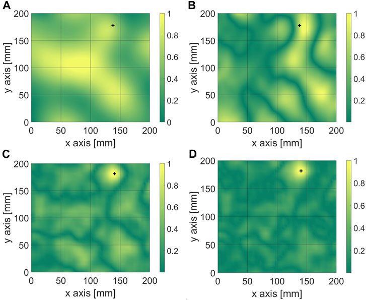
FIGURE 2. At a given t_i time, comparison between four different fields, all normalized by their respective maximal values: (A) Displacement field w(x, y, t_i), (B) First-order spatial derivative of the displacement field, $\frac{\partial w}{\partial x}+\frac{\partial w}{\partial y}$, (C) Second-order spatial derivative of the displacement field, $\frac{{\partial }^{2}w}{\partial x^2}+\frac{{\partial }^{2}w}{\partial y^2}$. (D) Reconstructed force field using Eq. 2. A + black sign indicates the actual position of the sound source at t_i.

3.2 Identification of optimal parameters

Images are recorded by the high-speed camera at a specific rate (in frames per second, fps) that has to be theoretically at least twice the excitation frequency following Shannon’s theorem. Since the camera’s storage capacity is limited to 21,841 images at full resolution (1,024 × 1,024 pixels), a large fps goes with a short acquisition duration. For all presented tests and results, the sensor’s resolution was set to 1,024 × 1,024 pixels and the camera’s sampling rate to 3,000 fps, with a maximum acquisition time of 7.28 s. All calculations were made using a personal computer equipped with an AMD Ryzen 5 4600H processor with a 3.0 GHz clock speed, 6 threads, and a 16 GB RAM. Finally, the to-be-reconstructed shape in this section is a heart drawn in front the membrane with the sound level calibrator.

Three main parameters can be considered to obtain meaningful results: (1) N_s the integer number of spatial steps S_x,y between two points of the scheme such that Δ_x,y = N_sS_x,y, (2) the threshold value above which the force amplitude is taken into account for the shape reconstruction; and (3) p_i the picture increment between two consecutive maps. S_x,y represents the spatial increment of the mesh grid with which the finite difference scheme is translated along the x and y-axis. In this work, S_x,y = p/2 = 2 mm. In Figure 1B, N_s = 1 on the left and N_s = 2 on the right. The influence of a variation in the membrane’s characteristics inputs (tension and surface mass) is also studied in this section. Lastly, except in the subsection that concerns the effect of time increment, all figures have been obtained by considering one picture out of fifty.

3.2.1 Spatial spacing used in the finite-difference scheme

The parameter N_s affects the overall size of the 5-point scheme used to calculate the spatial derivative of displacements. Thus, if the scheme is more extensive, fewer data are accessible (at the boundaries and over the whole measurement area), so the size of the force matrix is reduced. It leads to a coarser reconstitution of the shape inherent to the less dense mesh, which can be seen when comparing the four tested cases in Figure 3A. Calculation time to determine space-time varying loading is also related to N_s value: approximately 76 s are required to reconstruct the heart shape with N_s = 1, and 35 s with N_s = 2. Since the difference in the computation time with larger N_s values is less significant, and the shape is mainly recognizable with N_s = 2, this value conciliates precision and running time.

FIGURE 3

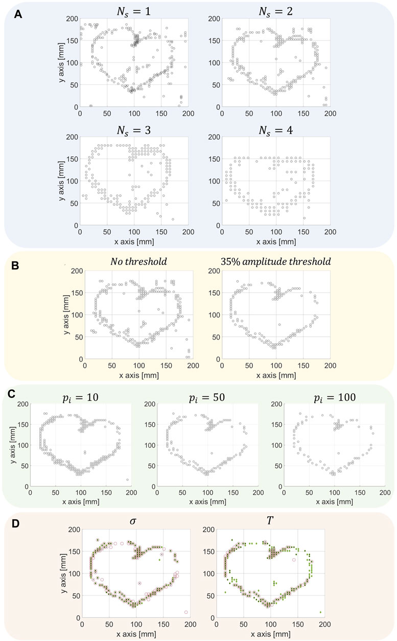
FIGURE 3. V1 (A) Effect of the spatial increment value N_s in the finite-difference scheme on the reconstruction of a heart shape. (B) Heart shape reconstructed without amplitude thresholding on the left and with a 35% amplitude threshold on the right.(C) Heart shape reconstructed with different increment p_i between the pictures used for inverse solving. (D) Heart shape reconstructed with an error of ±20% for the surface density (left) and the membrane’s tension (right)—red circles indicates a —20% error, green diamonds a +20% error, and black points are unbiased.

3.2.2 Force threshold definition

The quantitative values of the force amplitude are irrelevant for this work; a percentage of the highest amplitudes and their position are enough to reconstitute the shape drawn by the user. The threshold definition is based on a percentage of the most significant identified force amplitude over the acquisition time. Its optimal values were empirically determined and range between 15% and 45%. This threshold helps reduce noise-induced reconstruction artifacts and improves the precision of the reconstructed trajectories. By trial and error, a threshold of 35% of the largest estimated force amplitude is applied to every other figure in Section 3. As an example, the left figure in Figure 3B was obtained with no threshold (i.e., the localization of the identified maximum force amplitude over the measurement area is used to plot the loading’s trajectory). At the same time, the figure on the right was obtained with a 35% threshold of the maximum force amplitude estimated during measurement (the points plotted are only those that concern the localization of a loading magnitude larger than 35% of the largest recorded amplitude).

3.2.3 Time increment between consecutive images

For a full acquisition time of 7.28 s, 21,841 images are recorded by the camera at a rate of 3,000 frames per second (one picture is taken each 0.3 ms). However, not all data is necessarily required to get a satisfying result. Figure 3C compares the results for different time increments (one picture out of 10, one picture out of 50, one picture out of 100). By varying the time increment p_i between available images, the total number of pictures to be processed also varies greatly. With an increment of p_i = 10, the heart on the left of Figure 3C is reconstructed with one picture out of ten, so a total of 2,185 pictures. The heart in the middle was obtained with only 437 pictures (one out of 50), and the heart on the right with 219 (one out of 100). The calculation times to calculate the force fields used to obtain the three figures of Figure 3C, from left to right, respectively, are 3.53 s, 0.85 s, and 0.57 s. A value of p_i = 50 leads to a well-defined shape and provides enough points to reconstruct quite complex writing with an acceptable time computation.

3.2.4 Influence of uncertainties on mechanical parameters values

A precise knowledge of mechanical properties is required for applying the force analysis technique for the usual identification purposes (Pézerat and Guyader, 1995; Pézerat and Guyader, 2000; Leclere and Pézerat, 2008). Variations in the membrane’s mechanical characteristics, such as an increase in tension value (T) or decrease in area density (σ), will result in a biased estimation of the force amplitude. In practice, variations of the membrane’s tension are quite inescapable, and the mass density and thickness of the membrane are challenging to evaluate perfectly. Figure 3D highlights that the drawn shape is still recognizable after the numerical reconstitution, even with the imprecision of ±20% on those inputs. In Figure 3D, the red circles indicate an imprecision of −20%, the green diamonds of +20%, and the black points are the reconstitution with the initial inputs. Additional tests proved that even if the area density value σ error can be as significant as 50%, the results obtained can still be considered acceptable. This is attributed to the fact that a relative identification of the force amplitude is sought, making the identification process less prone to errors in mechanical parameters.

3.3 Additional examples using optimal parameters

Using the set of optimal parameters previously identified (N_s = 2, p_i = 50, 15% ≤ threshold $\le 45\%$), various hand gestures using both acoustic sources are recovered. Figure 4 provides several examples. The word ‘net’ (Figure 4A) and the letter ‘Σ’ (Figure 4B) were written with the acoustic calibrator (1,000 Hz), and reconstructed with a force amplitude threshold of 40% and 20%, respectively. Since the sound pressure level calibrator has a fixed frequency, a smartphone was used to conduct tests at a frequency empirically defined as half of the frequency of the calibrator. A smartphone generating a sine wave at a frequency of 500 Hz was thus used to draw the letter ‘P’ (Figure 4C) and the shape ★ (Figure 4D). The threshold value was also set to 20%. Most shapes, especially the simplest ones, are easily recognizable, such as ‘P’ and ‘Σ’.

FIGURE 4

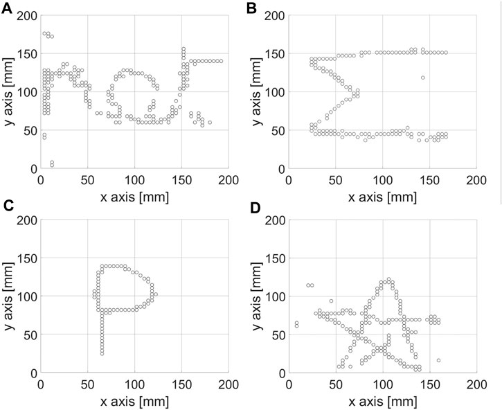
FIGURE 4. Different shapes reconstituted with optimal parameters N_s = 2, p_i = 50 and an adapted force amplitude threshold: (A) Word ‘net’, 40% threshold, (B) Letter “Σ”, 20% threshold, (C) Letter ‘P’, 20% threshold, (D) Shape ★, 20% threshold.

4 Discussion

Following the provided example, one of the possible applications of the proposed work would be an acoustic pencil concept with a membrane board. Regarding the acoustic pencil, and since the idea was initially implemented with a sound level calibrator, using a smartphone as an acoustic source for the presented concept is successful. With a unique device, the smartphone gives the ability to choose various excitation frequencies that extend the range of acquisition rate that can be used with the camera. Drawing a large shape or a long word inherently takes time. Reaching lower fps allows a longer acquisition time (for a fixed memory) and reduces the technical requirements. Moreover, a smartphone is an accessible resource; no specific application is required. On the other hand, the reconstruction of the drawn shapes is currently divided into two stages. First, the acoustic source moves along the membrane while images are acquired with a high-speed camera; images are then post-treated to obtain the displacement field over time and apply the force analysis technique to retrieve the force maps.

If real-time implementation were contemplated, direct processing of acquired images would be required. GPU or FPGA boards could be used to acquire the images one by one (and not after recording the complete film), directly perform parallel processing of the different parts of the image to perform the calculations and display the instantaneous result. In such a case, this proof of concept could finally lead to the viable concept of a contactless membrane board.

However, starting from this proof of concept, several points have to be investigated in future works. The setup of a large and possibly square membrane is under consideration to eliminate possible reflection effects from the surrounding frame in the case of this circular membrane. Also, a reference to obtain the exact position of the sound source is required to estimate the precision of the identification. Two options will be considered. The first is an infrared touchscreen overlay, a frame within which the source can be located. However, the separation distance between the membrane and this frame must be fixed. The second option is a robotic arm with prescribed trajectories, which can help evaluate trajectory identification in 3D. These elements will be combined with a multi-factor evaluation, including the influence of the drawing speed, the effect of source-to-membrane separation, and source strength and frequency requirements.

This work combines time-resolved full-field vibration measurements on a circular membrane with the force analysis technique to recover pressure loading as a function of space and time. Simple hand gestures that correspond to the drawing of a Greek letter (Σ), a capital letter (P), two shapes (♡, ⋆), and a 3-letter word (net) are effectively recovered. This work provides an example of how an identification technique can be used qualitatively rather than in the more usual quantitative way. However, if quantitative identification is sought, combining the force analysis technique with full-field vibration measurements on a membrane allows time-space identification of an acoustic loading and opens exciting perspectives that could be applied in several fields. Three examples are (1) the characterization of membrane-like acoustic metamaterials (Huang et al., 2016); (2) the time-space reconstruction of a turbulent boundary layer loading on a membrane (O’Donoughue et al., 2019b), which could help identify the spatial decay coefficients and the power spectral density of this specific loading, and (3) application in musical acoustics, especially the characterization of membranophones including the interaction between the performer and its instrument. In the latter case, the reconstruction of a time-space-varying mechanical loading would be considered, providing another research direction. As a final and inspiring example that mixes metamaterials and musical acoustics, high-speed laser interferometry measurements were used in (Bader et al., 2019) to characterize the effect brought by a modified frame drum inspired by metamaterials, showing enlarged variability in terms of timbre and musical articulations compared with a regular drum.

Data availability statement

The raw data supporting the conclusion of this article will be made available by the authors, without undue reservation.

Author contributions

AM: Data curation, Formal Analysis, Investigation, Visualization, Writing–review and editing. OR: Conceptualization, Funding acquisition, Investigation, Project administration, Resources, Supervision, Visualization, Writing–original draft. MM: Data curation, Methodology, Supervision, Writing–review and editing.

Funding

The author(s) declare financial support was received for the research, authorship, and/or publication of this article. This work is supported by a NSERC Discovery Grant (Visible and infrared deflectometry for contactless and full-field vibration measurements). The additional support of International Research Project - Centre Acoustique Jacques Cartier is also acknowledged.

Acknowledgments

Prof. Alain Berry and Dr. P. O’Donoughue are thanked for fruitful discussions at the early stage of this work.

Conflict of interest

The authors declare that the research was conducted in the absence of any commercial or financial relationships that could be construed as a potential conflict of interest.

The author(s) declared that they were an editorial board member of Frontiers, at the time of submission. This had no impact on the peer review process and the final decision.

Publisher’s note

All claims expressed in this article are solely those of the authors and do not necessarily represent those of their affiliated organizations, or those of the publisher, the editors and the reviewers. Any product that may be evaluated in this article, or claim that may be made by its manufacturer, is not guaranteed or endorsed by the publisher.

References

Ablitzer, F., Pézerat, C., Génevaux, J.-M., and Bégué, J. (2014). Identification of stiffness and damping properties of plates by using the local equation of motion. J. Sound Vib. 333, 2454–2468. doi:10.1016/j.jsv.2013.12.013

CrossRef Full Text | Google Scholar

Bader, R., Fischer, J., Münster, M., and Kontopidis, P. (2019). Metamaterials in musical acoustics: a modified frame drum. J. Acoust. Soc. Am. 145, 3086–3094. doi:10.1121/1.5102168

PubMed Abstract | CrossRef Full Text | Google Scholar

Burke, J., Pak, A., Höfer, S., Ziebarth, M., Roschani, M., and Beyerer, J. (2023). Deflectometry for specular surfaces: an overview. Adv. Opt. Technol. 12. doi:10.3389/aot.2023.1237687

CrossRef Full Text | Google Scholar

Chen, G., and Lu, Y. (2020). Fast-moving sound source tracking with relative Doppler stretch. IEEE Access 8, 221269–221277. doi:10.1109/ACCESS.2020.3043270

CrossRef Full Text | Google Scholar

Chiariotti, P., Martarelli, M., and Castellini, P. (2019). Acoustic beamforming for noise source localization – reviews, methodology and applications. Mech. Syst. Signal Process. 120, 422–448. doi:10.1016/j.ymssp.2018.09.019

CrossRef Full Text | Google Scholar

Devivier, C., Pierron, F., and Wisnom, M. (2012). Damage detection in composite materials using deflectometry, a full-field slope measurement technique. Compos. Part A Appl. Sci. Manuf. 43, 1650–1666. doi:10.1016/j.compositesa.2011.11.009

CrossRef Full Text | Google Scholar

Djamaa, M., Ouelaa, N., Pézerat, C., and Guyader, J. (2007). Reconstruction of a distributed force applied on a thin cylindrical shell by an inverse method and spatial filtering. J. Sound Vib. 301, 560–575. doi:10.1016/j.jsv.2006.10.021

CrossRef Full Text | Google Scholar

Drafts, B. (2001). Acoustic wave technology sensors. IEEE Trans. Microw. theory Tech. 49, 795–802. doi:10.1109/22.915466

CrossRef Full Text | Google Scholar

Huang, T., Shen, C., and Jing, Y. (2016). Membrane- and plate-type acoustic metamaterials. J. Acoust. Soc. Am. 139, 3240–3250. doi:10.1121/1.4950751

PubMed Abstract | CrossRef Full Text | Google Scholar

Kaufmann, R., Ganapathisubramani, B., and Pierron, F. (2019). Full-field surface pressure reconstruction using the virtual fields method. Exp. Mech. 59, 1203–1221. doi:10.1007/s11340-019-00530-2

CrossRef Full Text | Google Scholar

Kent, J. (2010). New touch technology from time reversal acoustics: a history. IEEE Int. Ultrason. Symp., 1173–1178. doi:10.1109/ULTSYM.2010.5935502

CrossRef Full Text | Google Scholar

Knapp, C., and Carter, G. (1976). The generalized correlation method for estimation of time delay. IEEE Trans. Acoust. Speech, Signal Process. 24, 320–327. doi:10.1109/TASSP.1976.1162830

CrossRef Full Text | Google Scholar

Leclère, Q., Ablitzer, F., and Pézerat, C. (2014). “Identification of loads of thin structures with the corrected force analysis technique: an alternative to spatial filtering regularization,” in Isma 2014 - leuven, Belgium.ISMA, Belgium.

Google Scholar

Leclère, Q., Ablitzer, F., and Pézerat, C. (2015). Practical implementation of the corrected force analysis technique to identify the structural parameter and load distributions. J. Sound Vib. 351, 106–118. doi:10.1016/j.jsv.2015.04.025

CrossRef Full Text | Google Scholar

Leclere, Q., and Pézerat, C. (2008). Time domain identification of loads on plate-like structures using an array of acoustic velocity sensors. J. Acoust. Soc. Am. 123, 3175. doi:10.1121/1.2933259

CrossRef Full Text | Google Scholar

Leclère, Q., and Picard, C. (2015). Acoustic beamforming through a thin plate using vibration measurements. J. Acoust. Soc. Am. 137, 3385–3392. doi:10.1121/1.4921272

PubMed Abstract | CrossRef Full Text | Google Scholar

Lecoq, D., Pézerat, C., Thomas, J., and Bi, W. (2014). Extraction of the acoustic component of a turbulent flow exciting a plate by inverting the vibration problem. J. Sound Vib. 333, 2505–2519. doi:10.1016/j.jsv.2014.02.003

CrossRef Full Text | Google Scholar

Logan, P., Avitabile, P., and Dodson, J. (2020). Reconstruction of external forces beyond measured points using a modal filtering decomposition approach. Exp. Tech. 44, 113–125. doi:10.1007/s40799-019-00340-0

CrossRef Full Text | Google Scholar

Martin, N., and Leehey, P. (1977). Low wavenumber wall pressure measurements using a rectangular membrane as a spatial filter. J. Sound Vib. 52, 95–120. doi:10.1016/0022-460X(77)90391-1

CrossRef Full Text | Google Scholar

Meng, F., Li, Y., Masiero, B., and Vorländer, M. (2019). Signal reconstruction of fast moving sound sources using compressive beamforming. Appl. Acoust. 150, 236–245. doi:10.1016/j.apacoust.2019.02.012

CrossRef Full Text | Google Scholar

O’Donoughue, P. (2020). Identification de Chargements Dynamiques sur des Structures Planes par Déflectométrie Optique et la Méthode des Champs Virtuels. Ph.D. thesis, Université de Sherbrooke

Google Scholar

O’Donoughue, P., Gautier, F., Meteyer, E., Durand-Texte, T., Secail-Geraud, M., Foucart, F., et al. (2023). Comparison of three full-field optical measurement techniques applied to vibration analysis. Sci. Rep. 13, 3261–3310. doi:10.1038/s41598-023-30053-9

PubMed Abstract | CrossRef Full Text | Google Scholar

O’Donoughue, P., Robin, O., and Berry, A. (2019a). “Inference of random excitations from contactless vibration measurements on a panel or membrane using the virtual fields method,” in Flinovia—flow induced noise and vibration issues and aspects-II. Editors E. Ciappi, S. De Rosa, F. Franco, J. Guyader, S. A. Hambric, R. C. K. Leunget al. (Cham: Springer International Publishing), 357–372.

Google Scholar

O’Donoughue, P., Robin, O., and Berry, A. (2019b). Time-space identification of mechanical impacts and distributed random excitations on plates and membranes. Proc. Institution Mech. Eng. Part C J. Mech. Eng. Sci. 233, 6436–6447. doi:10.1177/0954406219839094

CrossRef Full Text | Google Scholar

O’Donoughue, P., Robin, O., Rouard, K., Le Bot, A., and Berry, A. (2021). Post-processing deflectometry grid images using particle image velocimetry analysis. J. Vib. Acoust. 144, 034501. doi:10.1115/1.4052943

CrossRef Full Text | Google Scholar

Pézerat, C., and Guyader, J. (1995). Two inverse methods for localisation of external sources exciting a beam. Acta Acust. 3, 1–10.

Google Scholar

Pézerat, C., and Guyader, J. (2000). Force analysis technique: reconstruction of force distribution on plates. Acustica united Acta Acustica 86, 322–332.

Google Scholar

Phares, R. (2016). Acoustic touchscreen technology. Cham: Springer International Publishing. doi:10.1007/978-3-319-14346-0_206

CrossRef Full Text | Google Scholar

Quaegebeur, N., Padois, T., Gauthier, P., and Masson, P. (2016). Enhancement of time-domain acoustic imaging based on generalized cross-correlation and spatial weighting. Mech. Syst. Signal Process. 75, 515–524. doi:10.1016/j.ymssp.2015.12.012

CrossRef Full Text | Google Scholar

Reis, S., Correia, V., Martins, M., Barbosa, G., Sousa, R., Minas, G., et al. (2010). Touchscreen based on acoustic pulse recognition with piezoelectric polymer sensors. IEEE Int. Symposium Industrial Electron. (IEEE), 516–520.

CrossRef Full Text | Google Scholar

Renzi, C., Pézerat, C., and Guyader, J. (2013). Vibratory source identification by using the finite element model of a subdomain of a flexural beam. J. Sound Vib. 332, 545–562. doi:10.1016/j.jsv.2012.09.003

CrossRef Full Text | Google Scholar

Robin, O., Berry, A., Amédin, C. K., Atalla, N., Doutres, O., and Sgard, F. (2019). Laboratory and in situ sound absorption measurement under a synthetized diffuse acoustic field. Build. Acoust. 26, 223–242. doi:10.1177/1351010X19870307

CrossRef Full Text | Google Scholar

Robin, O., O’Donoughue, P., Berry, A., Farley, V., and Prithipaul, K. (2021). Full field vibration measurements on a cantilever beam under impact using visible and infrared deflectometry. Appl. Acoust. 183, 108294. doi:10.1016/j.apacoust.2021.108294

CrossRef Full Text | Google Scholar

Sanchez, J., and Benaroya, H. (2014). Review of force reconstruction techniques. J. Sound Vib. 333, 2999–3018. doi:10.1016/j.jsv.2014.02.025

CrossRef Full Text | Google Scholar

Singh, B., and Nanda, B. (2012). Estimation of damping in layered welded structures with unequal thickness. Shock Vib. 19, 1463–1475. doi:10.1155/2012/237605

CrossRef Full Text | Google Scholar

Staacks, S., Hütz, S., Heinke, H., and Stampfer, C. (2018). Advanced tools for smartphone-based experiments: phyphox. Phys. Educ. 53, 045009. doi:10.1088/1361-6552/aac05e

CrossRef Full Text | Google Scholar

Sur, T., and Grédiac, M. (2016). Influence of the analysis window on the metrological performance of the grid method. J. Math. Imaging Vis. 56, 472–498. doi:10.1007/s10851-016-0650-z

CrossRef Full Text | Google Scholar

Yin, S., Cui, Z., Fu, J., and Kundu, T. (2019). Acoustic source localization in heterogeneous media. Ultrasonics 99, 105957. doi:10.1016/j.ultras.2019.105957

PubMed Abstract | CrossRef Full Text | Google Scholar