 Emanuele Riva
 Matheus I. N. Rosa
 Yuning Guo2
 Massimo Ruzzene
- 1Department of Mechanical Engineering, Politecnico di Milano, Milano, Italy
- 2Department of Mechanical Engineering, University of Colorado Boulder, Boulder, CO, United States
We investigate the dynamics of acoustic waveguides with time-varying Helmholtz resonators and the ensuing wave propagation features. We focus on the numerical modeling of such a system with emphasis on the time-varying dispersion properties and emerging wave phenomena due to slow time modulation. We show that a propagating wave packet experiences a transformation that preserves the wavenumber content, resulting in frequency conversion that follows the time evolution of the dispersion bands. The conditions for such a transformation to be “adiabatic” are derived analytically, which allows the identification of the limiting modulation speed required to avoid undesired reflections or mode conversions. The predictions from the dispersion investigations are confirmed by time-domain numerical simulations, which illustrate the possibilities for frequency conversion and temporal signal compression or decompression of impinging signals. The framework presented herein may open new avenues in the context of time-varying phonic waveguides, with possible applications in communication, sound isolation, and frequency conversion.
1 Introduction
The extensive research in metamaterials has investigated intriguing properties to functionally control wave propagation within different physical domains. Various implementations in optical, elastic, and acoustic systems showcase phenomena produced by periodic tessellations of Bragg-scattering or locally-resonant units, which define different bandgap formation mechanisms (Hussein et al., 2014; Cummer et al., 2016; Kadic et al., 2019; Oudich et al., 2023). Following this concept, a number of wave manipulation strategies have emerged to produce attenuation (Liu et al., 2000), localization (Hu et al., 2021), and mode-conversion (Dong et al., 2022), which are of particular relevance for sound and vibration isolation purposes. Other configurations rely on the careful manipulation of spatial symmetries in the creation of back-scattering immune topological waveguides (Ma et al., 2019), including elastic/acoustic analogs to the quantum spin Hall (QSH) (Süsstrunk and Huber, 2015; Miniaci et al., 2018) and quantum valley Hall (QVH) (Pal and Ruzzene, 2017) effects, for example. Another line of work takes advantage of metamaterials with gradually varying units, which are known to support slow waves (Tsakmakidis et al., 2007; Wang et al., 2023) produced by a gradual decrease of the wave’s speed in space, and which may be useful in applications such as energy harvesting (De Ponti et al., 2020) and enhanced sensing (Chen et al., 2014). Acoustic cloaks (Norris, 2008), rainbow trappers (De Ponti et al., 2021), and lenses (Allam et al., 2021) are additional examples where spatial variations of the underlying medium properties are key in providing some degree of wave control.
All the examples above are induced by a modulation of the underlying media in space. However, wave propagation in spatially periodic or spatially varying systems is constrained by frequency-invariant dispersion characteristics. In contrast, time-modulated metamaterials are excellent candidates to broaden the wave control opportunities in the context of metamaterial-based waveguiding. For instance, non-reciprocal wave propagation (Trainiti and Ruzzene, 2016; Marconi et al., 2020), parametric amplification (Trainiti et al., 2019), temporal pumping (Grinberg et al., 2020; Xu et al., 2020; Xia et al., 2021), and temporal waveguiding (Pacheco-Peña and Engheta, 2020b; Santini and Riva, 2022) are behaviors that cannot be met by linear time-invariant interactions. Experiments on this matter have propelled this research topic, establishing itself as an attractive field during active times in phononics (Zangeneh-Nejad and Fleury, 2019).
In this context, we present a framework for the study of wave propagation in time-modulated acoustic metamaterials within the context of an adiabatic theorem. Our analysis is inspired by previous studies on adiabatic transformations of standing modes (Xia et al., 2021), and on adiabatic wave steering in spring-mass lattices (Santini and Riva, 2022). Here, we explore an acoustic waveguide endowed with Helmholtz resonators whose neck cross-section is modulated in time to produce a time-varying resonant frequency. We show that an incident wave packet propagating through the time-varying waveguide undergoes a wavenumber-invariant frequency conversion that follows the time evolution of the dispersion bands. Through the adiabatic theorem, we show that fast, or non-adiabatic, modulations produce leaks from the incident wave packet toward other wave modes. Through this framework, we compute a limiting condition for the modulation velocity which produces frequency conversion through a scattering-free process and we identify the transition between adiabatic and non-adiabatic processes. Supported by the derived adiabatic conditions, our numerical results reveal possibilities for frequency conversion and temporal signal compression or decompression, which may define novel functionalities of metamaterial waveguides enabled by smooth temporal modulations which may otherwise be difficult to realize via purely mechanical or electromechanical configurations (Xia et al., 2021).
This paper is organized as follows. The theoretical aspects are discussed in Section 2, starting from the derivation of the equations of motion and with emphasis on the dispersion analysis and the adiabatic theorem. In Section 3, we report a number of relevant case-studies, where time modulation is tailored to control frequency and mode conversion. Concluding remarks are presented in Section 4.
2 Acoustic waveguides with time-varying resonators: modeling and solution methods
In this section, we describe the modeling of the one-dimensional (1D) acoustic waveguide endowed with time-varying Helmholtz resonators. We first derive the equations of motion of the coupled system, followed by a homogenization in the long-wavelength limit which allows for analytical expressions of the dispersion relations in the absence of time modulation. Finally, we describe the adiabatic conditions for transformations induced by slow time modulation of the resonators’ properties, which delineates the transition between frequency conversion with and without energy scattering toward undesired wave modes.
2.1 Equations of motion
We consider a 1D acoustic waveguide of constant cross-section area A, featuring a period array of Helmholtz resonators of volume V, spaced by a distance a (Figure 1). The resonators have a neck length l and neck area Ar(t), the latter assumed to be mechanically varied in time. The wave equation for the acoustic waveguide is expressed as Kinsler et al. (2000):
where
where δ(x − xj) is the delta function that accounts for the assumed point-wise action of the jth resonator placed at xj. Substitution of 3 into 1 yields the equations of motion of the waveguide coupled with those of the resonators:
where m = ρArl′ and
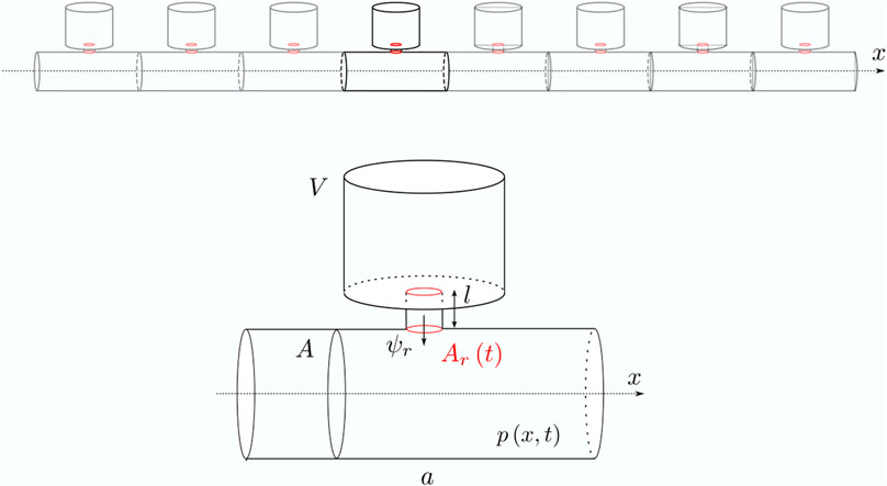
FIGURE 1. Schematic of the waveguide endowed with Helmholtz resonators, along with a zoomed view of the unit cell. The neck cross-section area Ar, highlighted in red, is modulated in time, while the other parameters are kept constant.
2.2 Dispersion calculation in the subwavelength regime
In order to investigate wave motion in the considered system and carry out analytical derivations, we now consider the homogenized version of Eq. 3, whereby the resonators are continuously distributed through the pipe:
Here, both
where μ = V/aA is the volume ratio, i.e., the ratio between the volume enclosed in the resonator’s chamber and the volume of the unit cell’s pipe segment. Eq. 7 can be directly solved for
Note that for any real-valued wavenumber κ, there are four solutions that define wave modes propagating in the pipe. The dispersion relation
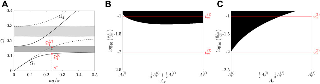
FIGURE 2. (A) Dispersion relation before (solid line) and after (dashed line) time-modulation. The gray boxes highlight the corresponding variation of the gap limits. The energy, provided with a central frequency
While here the area
2.3 Adiabatic transformations for slow temporal modulations
To investigate the time-varying dynamics caused by slow temporal variations of the area Ar, Eq. 4 is written in a first-order differential form by imposing only the wavenumber κ:
where
This first-order differential form resembles Schrodinger’s equations for quantum states where the adiabatic theorem is classically established [see for example, the book by Griffiths and Schroeter (2018), and also employed in multiple following studies due to its convenience in deriving adiabatic conditions (Amin, 2009; Tong, 2010). The ansatz
where
where
Since the second term on the right-hand side (obtained through integration by parts) is negligible (Ibáñez and Muga, 2014), we arrive at the following condition:
The condition in Eq. 12 is employed to analyze the coupling between the imposed wave mode and the other modes which may be involved in the solution. The condition must be evaluated for a given pair of wave modes and a certain imposed wavenumber. To exemplify, we consider the imposed wavenumber k* and solution Ω1 marked in Figure 2A, and we quantify the coupling to the solution Ω2 and to the left-propagating solution Ω−1 = −Ω1 in Figures 2B, C, respectively. We evaluate the norm in Eq. 12 as a function of Ar and its rate of change (i.e., modulation speed) vm = ∂Ar/∂t, marking with black the regions that surpass a chosen threshold value of 0.01. The plots, therefore, serve as maps which mark adiabatic (white) and non-adiabatic (black) regions as a function of Ar and vm. Two horizontal lines for representative velocity values
3 Numerical results
In this section, we present a few case studies to elucidate the role of time modulation in the considered acoustic metamaterials, with emphasis on frequency conversion, mode conversion, and the derived adiabatic conditions. The results are obtained through numerical simulations performed through a finite difference time domain (FDTD) algorithm, where the partial derivatives in Eq. 3 are discretized through a central difference approximation, and absorbing conditions are added to the boundaries to mitigate reflections. For simplicity, we employ a piecewise linear variation of the neck cross-section area:
Where ti and tf are the start and finish time instants for the modulation, and vm is the constant modulation velocity. In the simulations, a sinusoidal wave packet with n = 30 periods is imposed through a prescribed velocity to the left end of a finite waveguide of length L. We remark that the wavepacket propagates at a speed given by the group velocity cg = ∂ω/∂κ, which is evaluated at the impinging wavenumber κ and angular frequency
The time history relative to example (i) is displayed in Figure 3A. The excitation is provided with a central frequency
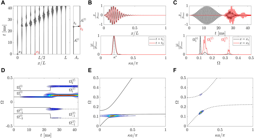
FIGURE 3. (A) Wavefield
To better illustrate the frequency transformations, we present a frequency spectrogram in Figure 3D, which is evaluated by windowing the pressure field
A cleaner frequency conversion and signal compression are demonstrated in the second example (ii) corresponding to a modulation velocity
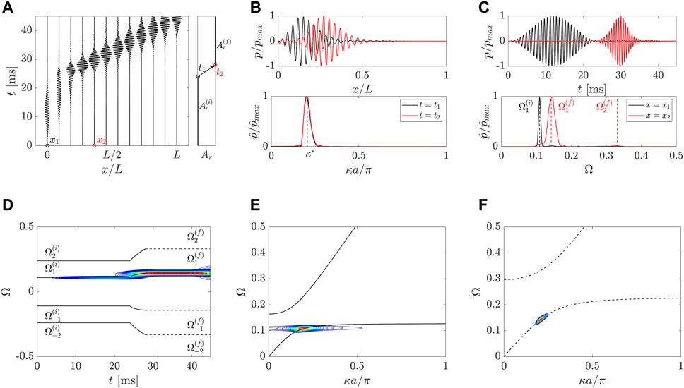
FIGURE 4. (A) Wavefield
4 Conclusion
In this paper, we have explored the dynamics of acoustic metamaterials endowed with time-varying Helmholtz resonators. When a sound wave propagates simultaneously to a temporal modulation, the wave packet experiences a frequency conversion dictated by the underlying dispersion, which may result in signal compression or dilation. If the speed of the modulation is fast, or non-adiabatic, the time evolution of the wave packet can be accompanied by energy scattering to other wave modes. In contrast, sufficiently slow modulations can frequency transform the impinging wave in an adiabatic manner and without any energy leak to the other dispersion branches. We have established the limiting condition for the modulation speed to distinguish between adiabatic and non-adiabatic processes. The developed framework, illustrated through selected numerical case studies, is generally applicable to a variety of time-varying metamaterial systems. Therefore, the presented results may open new opportunities in time-varying acoustics with application to signal processing, sound isolation, and energy conversion. Future investigations will focus on the experimental validation of the concepts herein explored, where time-varying resonators can be achieved through mechanical opening and closure of the apertures. Similar approaches have been used in the context of acoustic topological pumping for example, by the relative translation of two incommensurate waveguides (Cheng et al., 2020) or dynamic boundary changes through rotation mechanisms (Xu et al., 2020).
Data availability statement
The raw data supporting the conclusion of this article will be made available by the authors, without undue reservation.
Author contributions
ER: Formal Analysis, Investigation, Software, Visualization, Writing–original draft. MRo: Conceptualization, Investigation, Software, Visualization, Writing–original draft. YG: Conceptualization, Investigation, Software, Visualization, Writing–original draft, Writing–review and editing. MRu: Conceptualization, Funding acquisition, Writing–review and editing.
Funding
The author(s) declare that no financial support was received for the research, authorship, and/or publication of this article.
Conflict of interest
The authors declare that the research was conducted in the absence of any commercial or financial relationships that could be construed as a potential conflict of interest.
The authors MRu and ER declared that they were editorial board members of Frontiers at the time of submission. This had no impact on the peer review process and the final decision.
Publisher’s note
All claims expressed in this article are solely those of the authors and do not necessarily represent those of their affiliated organizations, or those of the publisher, the editors and the reviewers. Any product that may be evaluated in this article, or claim that may be made by its manufacturer, is not guaranteed or endorsed by the publisher.
Supplementary material
The Supplementary Material for this article can be found online at: https://www.frontiersin.org/articles/10.3389/facou.2023.1271221/full#supplementary-material
References
Allam, A., Sabra, K., and Erturk, A. (2021). Sound energy harvesting by leveraging a 3d-printed phononic crystal lens. Appl. Phys. Lett. 118, 103504. doi:10.1063/5.0030698
Amin, M. H. (2009). Consistency of the adiabatic theorem. Phys. Rev. Lett. 102, 220401. doi:10.1103/physrevlett.102.220401
Chen, Y., Liu, H., Reilly, M., Bae, H., and Yu, M. (2014). Enhanced acoustic sensing through wave compression and pressure amplification in anisotropic metamaterials. Nat. Commun. 5, 5247. doi:10.1038/ncomms6247
Cheng, W., Prodan, E., and Prodan, C. (2020). Experimental demonstration of dynamic topological pumping across incommensurate bilayered acoustic metamaterials. Phys. Rev. Lett. 125, 224301. doi:10.1103/physrevlett.125.224301
Cummer, S. A., Christensen, J., and Alù, A. (2016). Controlling sound with acoustic metamaterials. Nat. Rev. Mater. 1, 16001–16013. doi:10.1038/natrevmats.2016.1
De Ponti, J. M., Colombi, A., Riva, E., Ardito, R., Braghin, F., Corigliano, A., et al. (2020). Experimental investigation of amplification, via a mechanical delay-line, in a rainbow-based metamaterial for energy harvesting. Appl. Phys. Lett. 117, 143902. doi:10.1063/5.0023544
De Ponti, J. M., Iorio, L., Riva, E., Ardito, R., Braghin, F., and Corigliano, A. (2021). Selective mode conversion and rainbow trapping via graded elastic waveguides. Phys. Rev. Appl. 16, 034028. doi:10.1103/physrevapplied.16.034028
Dong, H.-W., Zhao, S.-D., Oudich, M., Shen, C., Zhang, C., Cheng, L., et al. (2022). Reflective metasurfaces with multiple elastic mode conversions for broadband underwater sound absorption. Phys. Rev. Appl. 17, 044013. doi:10.1103/physrevapplied.17.044013
Griffiths, D. J., and Schroeter, D. F. (2018). Introduction to quantum mechanics. Cambridge: Cambridge University Press.
Grinberg, I. H., Lin, M., Harris, C., Benalcazar, W. A., Peterson, C. W., Hughes, T. L., et al. (2020). Robust temporal pumping in a magneto-mechanical topological insulator. Nat. Commun. 11, 974. doi:10.1038/s41467-020-14804-0
Hu, G., Tang, L., Liang, J., Lan, C., and Das, R. (2021). Acoustic-elastic metamaterials and phononic crystals for energy harvesting: A review. Smart Mater. Struct. 30, 085025. doi:10.1088/1361-665x/ac0cbc
Hussein, M. I., Leamy, M. J., and Ruzzene, M. (2014). Dynamics of phononic materials and structures: Historical origins, recent progress, and future outlook. Appl. Mech. Rev. 66. doi:10.1115/1.4026911
Ibáñez, S., and Muga, J. (2014). Adiabaticity condition for non-hermitian hamiltonians. Phys. Rev. A 89, 033403. doi:10.1103/physreva.89.033403
Kadic, M., Milton, G. W., van Hecke, M., and Wegener, M. (2019). 3d metamaterials. Nat. Rev. Phys. 1, 198–210. doi:10.1038/s42254-018-0018-y
Kinsler, L. E., Frey, A. R., Coppens, A. B., and Sanders, J. V. (2000). Fundamentals of acoustics. China: John Wiley & Sons.
Liu, Z., Zhang, X., Mao, Y., Zhu, Y., Yang, Z., Chan, C. T., et al. (2000). Locally resonant sonic materials. science 289, 1734–1736. doi:10.1126/science.289.5485.1734
Ma, G., Xiao, M., and Chan, C. T. (2019). Topological phases in acoustic and mechanical systems. Nat. Rev. Phys. 1, 281–294. doi:10.1038/s42254-019-0030-x
Marconi, J., Riva, E., Di Ronco, M., Cazzulani, G., Braghin, F., and Ruzzene, M. (2020). Experimental observation of nonreciprocal band gaps in a space-time-modulated beam using a shunted piezoelectric array. Phys. Rev. Appl. 13, 031001. doi:10.1103/physrevapplied.13.031001
Miniaci, M., Pal, R., Morvan, B., and Ruzzene, M. (2018). Experimental observation of topologically protected helical edge modes in patterned elastic plates. Phys. Rev. X 8, 031074. doi:10.1103/physrevx.8.031074
Norris, A. N. (2008). Acoustic cloaking theory. Proc. R. Soc. A Math. Phys. Eng. Sci. 464, 2411–2434. doi:10.1098/rspa.2008.0076
Oudich, M., Gerard, N. J., Deng, Y., and Jing, Y. (2023). Tailoring structure-borne sound through bandgap engineering in phononic crystals and metamaterials: A comprehensive review. Adv. Funct. Mater. 33, 2206309. doi:10.1002/adfm.202206309
Pacheco-Peña, V., and Engheta, N. (2020a). Antireflection temporal coatings. Optica 7, 323–331. doi:10.1364/optica.381175
Pacheco-Peña, V., and Engheta, N. (2020b). Temporal aiming. Light Sci. Appl. 9, 129. doi:10.1038/s41377-020-00360-1
Pal, R. K., and Ruzzene, M. (2017). Edge waves in plates with resonators: an elastic analogue of the quantum valley hall effect. New J. Phys. 19, 025001. doi:10.1088/1367-2630/aa56a2
Santini, J., and Riva, E. (2022). Elastic temporal waveguiding. New J. Phys. 25, 013031. doi:10.1088/1367-2630/acb45d
Sugino, C., Xia, Y., Leadenham, S., Ruzzene, M., and Erturk, A. (2017). A general theory for bandgap estimation in locally resonant metastructures. J. Sound Vib. 406, 104–123. doi:10.1016/j.jsv.2017.06.004
Süsstrunk, R., and Huber, S. D. (2015). Observation of phononic helical edge states in a mechanical topological insulator. Science 349, 47–50. doi:10.1126/science.aab0239
Tong, D. (2010). Quantitative condition is necessary in guaranteeing the validity of the adiabatic approximation. Phys. Rev. Lett. 104, 120401. doi:10.1103/physrevlett.104.120401
Trainiti, G., and Ruzzene, M. (2016). Non-reciprocal elastic wave propagation in spatiotemporal periodic structures. New J. Phys. 18, 083047. doi:10.1088/1367-2630/18/8/083047
Trainiti, G., Xia, Y., Marconi, J., Cazzulani, G., Erturk, A., and Ruzzene, M. (2019). Time-periodic stiffness modulation in elastic metamaterials for selective wave filtering: Theory and experiment. Phys. Rev. Lett. 122, 124301. doi:10.1103/physrevlett.122.124301
Tsakmakidis, K. L., Boardman, A. D., and Hess, O. (2007). ‘trapped rainbow’storage of light in metamaterials. Nature 450, 397–401. doi:10.1038/nature06285
Wang, X., Li, J., Yang, J., Chen, B., Liu, S., and Chen, Y. (2023). Compact acoustic amplifiers based on non-adiabatic compression of sound in metamaterial waveguides. Appl. Acoust. 204, 109246. doi:10.1016/j.apacoust.2023.109246
Xia, Y., Riva, E., Rosa, M. I., Cazzulani, G., Erturk, A., Braghin, F., et al. (2021). Experimental observation of temporal pumping in electromechanical waveguides. Phys. Rev. Lett. 126, 095501. doi:10.1103/physrevlett.126.095501
Xu, X., Wu, Q., Chen, H., Nassar, H., Chen, Y., Norris, A., et al. (2020). Physical observation of a robust acoustic pumping in waveguides with dynamic boundary. Phys. Rev. Lett. 125, 253901. doi:10.1103/physrevlett.125.253901
Keywords: acoustic metamaterials, time-varying waveguides, Helmholtz resonators, frequency conversion, time compression, adiabatic transformation
Citation: Riva E, Rosa MIN, Guo Y and Ruzzene M (2023) Adiabatic sound transport in acoustic waveguides with time-varying Helmholtz resonators. Front. Acoust. 1:1271221. doi: 10.3389/facou.2023.1271221
Received: 01 August 2023; Accepted: 28 September 2023;
Published: 11 October 2023.
Edited by:
Stefano Laureti, University of Calabria, ItalyReviewed by:
Marco Miniaci, Swiss Federal Laboratories for Materials Science and Technology, SwitzerlandMarco Ricci, University of Calabria, Italy
Copyright © 2023 Riva, Rosa, Guo and Ruzzene. This is an open-access article distributed under the terms of the Creative Commons Attribution License (CC BY). The use, distribution or reproduction in other forums is permitted, provided the original author(s) and the copyright owner(s) are credited and that the original publication in this journal is cited, in accordance with accepted academic practice. No use, distribution or reproduction is permitted which does not comply with these terms.
*Correspondence: Massimo Ruzzene, bWFzc2ltby5ydXp6ZW5lQGNvbG9yYWRvLmVkdQ==