Laboratory of Experimental Psychology, University of Leuven, Leuven, Belgium
Neural mechanisms underlying invariant behaviour such as object recognition are not well understood. For brain regions critical for object recognition, such as inferior temporal cortex (ITC), there is now ample evidence indicating that single cells code for many stimulus aspects, implying that only a moderate degree of invariance is present. However, recent theoretical and empirical work seems to suggest that integrating responses of multiple non-invariant units may produce invariant representations at population level. We provide an explicit test for the hypothesis that a linear read-out mechanism of a pool of units resembling ITC neurons may achieve invariant performance in an identification task. A linear classifier was trained to decode a particular value in a 2-D stimulus space using as input the response pattern across a population of units. Only one dimension was relevant for the task, and the stimulus location on the irrelevant dimension (ID) was kept constant during training. In a series of identification tests, the stimulus location on the relevant dimension (RD) and ID was manipulated, yielding estimates for both the level of sensitivity and tolerance reached by the network. We studied the effects of several single-cell characteristics as well as population characteristics typically considered in the literature, but found little support for the hypothesis. While the classifier averages out effects of idiosyncratic tuning properties and inter-unit variability, its invariance is very much determined by the (hypothetical) ‘average’ neuron. Consequently, even at population level there exists a fundamental trade-off between selectivity and tolerance, and invariant behaviour does not emerge spontaneously.
The ability to make abstraction of some aspects of observed events is critical for all animals. For example, if an exemplar of a particular species (e.g. tiger, or human) turns out to be very dangerous, then other exemplars of that same species might also be dangerous, even if encountered at a different place and time. While many examples can be given of how humans are superior to other species in terms of the degree of abstraction that can be made, a certain degree of abstraction is the hallmark of behaviour all around the animal world. Here we will mainly focus on a talent that is shared by many animals, namely the recognition of objects (‘Is this an animal, dog, my dog?’).
Object recognition is often invariant to the exact circumstances under which an object is perceived (Biederman and Bar, 2000
; Kravitz et al., 2008
). For example, we can recognize a dog irrespective of its retinal/spatial position, size, illumination, and viewpoint. Earlier models of object recognition stressed the need to construct an abstract, position-, size-, and viewpoint-invariant 3-D model of objects (Biederman, 1987
; Marr and Nishihara, 1978
). The question of how to construct invariant representations is also a central theme in computer vision (e.g. Khotanzad and Hong, 1990
; Lowe, 1999
, 2004
; Mundy and Zisserman, 1992
; Torres-Mendez et al., 2000
).
Limited Invariance of Single Neurons in the Primate Brain
Initially, neurophysiology studies were interpreted as showing that also the largest biological vision system, the primate brain, builds up invariant representations in cortical areas that are critical for object recognition, most notably the inferior temporal cortex (ITC; Logothetis and Sheinberg, 1996
). The most heavily studied attribute has been receptive field size, and older studies indeed reported very large receptive field sizes for ITC neurons (Desimone and Gross, 1979
; Desimone et al., 1984
; Gross et al., 1969
; Perrett et al., 1982
; Tovee et al., 1994
). However, more recent findings have revealed a different picture, with smaller receptive fields that convey relatively precise information about object position (DiCarlo and Maunsell, 2003
; Op de Beeck and Vogels, 2000
). The newer studies used smaller stimuli, and stimulus size was found to matter a lot: larger receptive fields are found with larger stimuli. Thus, the very large estimates in previous studies are most likely related to the use of very large stimuli, and in reality object representations in the monkey brain at the single unit level are not as invariant as the invariance that many computer vision systems aim to accomplish. It is interesting to note that recent theoretical neuroscience work has picked up these newer findings and explicitly included position coding as an intrinsic part of how objects are encoded and recognized (Edelman and Intrator, 2000
; Roudi and Treves, 2008
).
In addition to stimulus position, ITC neurons are also sensitive to other transformations, such as the size and viewpoint in which objects are shown (Ito et al., 1995
; Logothetis and Pauls, 1995
; Op de Beeck and Vogels, 2000
). Recently it was also found that the ideal of neurons with strong object selectivity together with high invariance is seldomly achieved in ITC cortex, as a trade off was found between the two at the level of single neurons (Zoccolan et al., 2007
). Neurons with high object selectivity tend to display less invariance compared to less selective neurons. This finding was observed for many dimensions for which an object recognition system might be tolerant, such as position, size, and clutter.
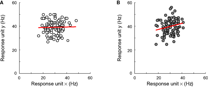
Figure 1
A illustrates the typical combination of selectivity for shape, position, and size at the level of single ITC neurons. This unit is selective for position (variation in colour in each panel), stimulus shape (lower responses in the middle panel compared to the left panel), and size (higher responses and larger receptive field in right panel compared to left panel). Two definitions of invariance have been used in studies of single-unit selectivity for multiple stimulus properties. The first definition focuses on ‘relative invariance’, which refers to a multidimensional tuning so that the preferences along one of the dimensions do not change when the value of another dimension is altered. The absolute magnitude of the responses might vary, but the order not (Sary et al., 1993
; Vogels and Orban, 1996
). For example, if we rank different object shapes or object sizes based on the response strength at one retinal position, then we see a similar preference for these object shapes or sizes at another retinal position (Figure 1
B; for empirical evidence, see Ito et al., 1995
; Op de Beeck and Vogels, 2000
). This ranking method is often used when at least one of the two dimensions is manipulated in a discrete manner (e.g. only two sizes or positions).
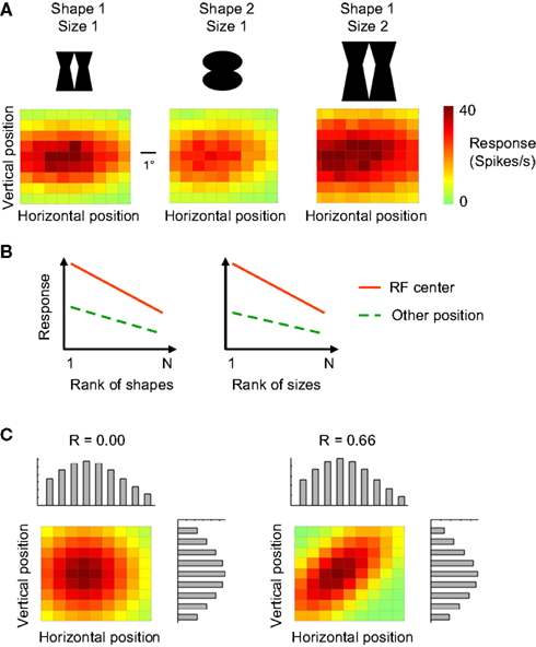
FigureÃÂ 1. Tuning properties of single neurons and definitions of invariance. (A) The tuning of one simulated neuron for retinal stimulus position (horizontal and vertical dimension in the colour matrices) as assessed with two shapes and two different sizes. The position and size sensitivity of this simulated neuron is representative for empirically measured tuning properties in monkey inferior temporal cortex. (B) The ‘relative invariance’ of tuning for multiple dimensions can be assessed by ranking stimuli that vary on one dimension based on the response strength at one value of a second dimension, and then verifying whether this stimulus preference is the same at another value of this second dimension. Here this phenomenon is illustrated with shape (left panel) or size (right panel) as the first dimension of which the values are being ranked, and retinal position as the second dimension. (C) The ‘independence’ of tuning for multiple dimensions can be assessed by comparing the joint 2-D tuning with the marginal tuning in which the tuning for one dimension is plotted averaged across all values of the other dimension. The left panel illustrated independence of tuning, the right panel a high degree of dependence.
A second definition of invariance is applicable in the case of continuously varying dimensions, and is based on the concept of independent or orthogonal tuning (Jones et al., 1987
; Kayaert et al., 2005
; Mazer et al., 2002
). If the tuning for two dimensions is independent or uncorrelated, then the 2-D tuning curve can be derived by multiplication of the two marginal distributions (the tuning for one dimension averaged across all values of the other dimension). An example of independent tuning is shown in Figure 1
C (left panel). The right panel of Figure 1
C shows a multidimensional tuning that violates independence. The concepts of relative invariance and independence are intertwined, as relative invariance will be limited or even non-existing if two dimensions are highly dependent.
Invariant Read-Out of Neural Population Response?
Some recent studies have moved away from single-neuron properties, and have focused on how the responses of multiple neurons can be read-out with linear classification methods. It has been suggested that linear classifiers reading the responses of inferior temporal neurons are able to make abstraction of to-be-ignored dimensions like position and size (Hung et al., 2005
), despite the selectivity for these dimensions at the single-neuron level as illustrated above. Similar conclusions have been reached for the human brain based on data obtained with functional magnetic resonance imaging (fMRI) and analyzed with multivariate techniques: The representations of objects in the human brain are sensitive to object position, but nevertheless allow the classification of objects across position (Schwarzlose et al., 2008
). Thus, despite the absence of completely invariant neurons or fMRI voxels, it might be possible to come to invariant recognition of objects based on the pattern of activity across multiple neurons or across multiple fMRI voxels.
While tempting to interpret these findings as showing that more invariance can be achieved at population level than at single-neuron level – thereby satisfying both the goals of selectivity and toleranceÃÂ – this may not be the correct conclusion. First, the population-level studies did not report the degree of invariance at the single-neuron or single-voxel level. For example, Hung et al. (2005)
used relatively small changes on the irrelevant dimensions (ID), and they might still have been in the relatively limited regime where neurons are indeed mostly invariant. Second, no study has investigated which non-invariant tuning functions of single neurons allow invariant read-out when neurons are combined and which do not. Not all non-invariant representations will allow invariant read-out, but some might (DiCarlo and Cox, 2007
). Obvious candidate tuning properties to consider are those investigated in the many single-unit studies of the past two decades: the degree of neural selectivity for the relevant stimulus-dimensions (e.g. object shape in the context of object recognition), for the to-be-ignored stimulus-dimensions (e.g. retinal position), and the degree of independence of the selectivity for these dimensions. Third, no attempt has been made to estimate how invariance at the population level depends on population characteristics such as pool size and correlated noise.
The Present Study
Here, we will study the effects of these aforementioned single unit and population characteristics on invariance at the population level. We will present a series of simulations with networks composed of units tuned along two dimensions according to a bivariate Gaussian distribution. We investigate how well a network trained to encode the value of the relevant dimension (RD) at one instance of the ID is able to generalize towards other instances of the ID. This is the way in which invariance has been tested in both the neuroimaging and neurophysiology literature (Hung et al., 2005
; Schwarzlose et al., 2008
). The aim of our simulations if thus to find out whether invariance is an automatically emerging property of classification at the population level when it is not explicitely trained. To explore effects of single unit and population characteristics, we manipulate the tuning width for the RD and ID, the degree of independence/covariance in the bivariate tuning and consider effects of pool size and correlated noise. Identification of a specific value in a 2-D stimulus space may seem fairly simple, but it can be generalized to the more general case of multiple dimensions. Further, to evaluate the ‘linear-population-invariance’ hypothesis, a well-defined and fully understood environment is better suited than real-life recognition – a field in which researchers still do not completely understand the complexity of the problem (see e.g. Pinto et al., 2008
). We will focus on the performance of a multivariate classification algorithm, i.e. linear support vector machines (SVMs), which receives a vector input formed by the activity pattern across multiple units (Hung et al., 2005
). Some neurophysiological studies have used simpler correlational analyses (e.g. Haxby et al., 2001
; Op de Beeck et al., 2008a
), or have compared a wide range of linear and non-linear classifiers (Cox and Savoy, 2003
; Haynes and Rees, 2006
; Kamitani and Tong, 2005
; Norman et al., 2006
). However, linear SVMs are widely used in recent studies, they are the most powerful classifier that is still neurally plausible (in contrast to non-linear methods, see Kamitani and Tong, 2005
), and this type of classifier was the one used in the recent studies that indicated that invariance can be achieved at the population level.
We will focus on three topics in our evaluation of the optimal tuning properties of neurons. First, how good is a network at identifying a target value on the RD among multiple distracter values? Second, how well does the network generalize to non-trained values on the ID? Finally, how does a network deal with potential changes in the dimensional relevance, so that the ID becomes relevant and vice versa (‘switching’)? The latter topic is especially important in the light of the aforementioned theoretical ideas that dimensions that are traditionally considered as irrelevant or even a nuisance for object identification might be relevant under certain circumstances (Edelman and Intrator, 2000
).
The results reveal, rather unsurprisingly, that the best network for identification and invariance is a network with narrow tuning for the RD and broad tuning for the ID. However, such a network performs poorly when the relevance of the two dimensions is switched, and this is not the tuning that has been found empirically. More intermediate and realistic combinations of tuning width of RD and ID reveal a trade-off between identification and invariance: better identification performance often leads to poorer invariance, and vice versa. The degree of independence in the bivariate tuning of units turned out to have surprisingly little effect on identification and invariance, as long as the deviations from independence among units were random (resulting in independence at the population level). However, while effects of idiosyncratic tuning properties and inter-unit variability may be averaged out at population level, the degree of invariance at population level is very much determined by the average unit, i.e. the (hypothetical) unit most representative for the pool. Consequently, our results show that even at population level there exists a fundamental trade-off between selectivity and tolerance. Perhaps surpringly, the implication is that sensitivity increases, but invariance decreases as a function of pool size, as is borne out by our data.
In this series of experiments, we simulated identification performance for several types of neural networks. All simulations, except for the introductory experiment, were run with an array of units tuned in a 2-D input space (X, Y). Unit tuning was 1-D in the introductory experiment. The preferred 2-D stimulus value of the units (i.e. their peak sensitivity), [E(x), E(y)], was randomly sampled from a bivariate uniform distribution encompassing the whole stimulus range used in the experiments. The tuning of each unit around this preferred value was defined by a 2-D Gaussian function (see e.g. Op de Beeck and Vogels, 2000
). The response of a unit as a function of the 2-D stimulus value, G(x, y), is given by Eq. 1:

with Rmax the maximum response of a unit (set to 40 spikes/s); MÃÂ the 2-D difference [xÃÂ −ÃÂ E(x) yÃÂ −ÃÂ E(y)] between the stimulus value and the value preferred by the unit; and COV the unit’s covariance matrix. Between units and simulations, the average unit tuning width (determined by the diagonal elements in COV) and average correlation (R, which is the covariance normalized for the squared tuning width, expressed in σ) were manipulated. Manipulations of this correlation are referred to as manipulations of ‘dependence’, to avoid confusion with our manipulation of correlated noise (see further). The details of these manipulations are described for each experiment in the respective section in ‘Results’.
To simulate the fact that neurons are noisy, the response of each unit on each trial was taken from a Poisson distribution with G(x,ÃÂ y) as mean. In experiment III, the responses of the network units are weakly correlated (i.e. they share some noise). This correlated noise was implemented by adding a random number, sampled from a standard normal distribution, to each unit response. This random number was also appropriately scaled, depending on the response strength of the unit. For each stimulus presentation, the random number was drawn anew. This implementation of correlated noise ensured that pair wise correlations of the responses of all network units were approximately identical (i.e. 0.15). The correlated noise did not change the unit’s mean response, but increased the standard deviation to be slightly higher than Poisson noise, consistent with empirical observations in visual cortex (see e.g. Shadlen and Newsome, 1998
).
To measure the combined read-out of multiple units, linear SVM were used, implemented with the OSU-SVM toolbox based on the LIBSVM package (Schwarzlose et al., 2008
). The implemented problem was an identification task, explained in detail in section ‘Introductory Experiment’.
Introductory Experiment
To introduce the approach adopted in the simulations to follow, we first describe the results of a simple network in a straightforward identification experiment. In this experiment, the network was trained to discriminate a 1-D signal stimulus from a 1-D distracter stimulus. The signal stimulus remained constant throughout the whole experiment, while the distracter stimulus was randomly selected from a set of eight stimuli on each training run. This design is illustrated in Figure 2
A. Half of the distracter stimuli had a lower value than the signal stimulus while the other half had a higher value. This task may thus be thought off as decoding one specific value on a given dimension.
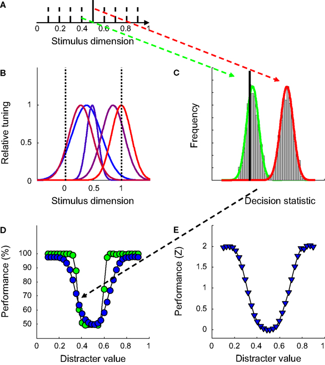
FigureÃÂ 2. The introductory experiment. (A) The network was trained to discriminate a 1-D signal (full black line) from a 1-D distracter, randomly selected from a set of eight distracters (dotted black lines) on each trial. (B)ÃÂ The Gaussian-shaped tuning functions for one particular network. (C)ÃÂ Estimates of the distribution of the decision statistic computed by the SVM for the signal (in red) and one particular distracter (in green) for one network, based on 1,000 trials. The full black line depicts the decision boundary used by the SVM to classify network responses. (D) Classification performance as a function of distracter value in the identification test. Green symbols indicate results for the network shown in Figure 1
B, blue symbols results averaged over 100 networks. (E) Normalized average classification performance as a function of distracter value. These data correspond to the blue symbols shown in panel (D). After normalization, performance is expressed in units of standard deviation above (or below) guess rate. Averaging over all 30 distracter values yields the sensitivity statistic used throughout the paper.
The networks trained to perform this task consisted of five units, the tuning of which is illustrated in Figure 2
B for one network. Peak sensitivity of these Gaussian-shaped tuning functions was randomly selected from a uniform distribution ranging between 0 and 1 (indicated by the dotted black lines in Figure 2
B). The width, expressed in σ, was randomly selected from a normal distribution with mean value 0.25 and standard deviation 0.1.
As in all experiments to follow, SVM-training consisted of 500 network-response patterns to both a signal and a range of distracter stimuli. In order to classify network responses, the SVM computes a decision statistic based on a linear combination of response patterns. Although responses of each unit are Poisson distributed (see Materials and Methods), the central limit theorem predicts that this decision statistic will be approximately normally distributed for any given stimulus. This can also be seen in Figure 2
C. Estimates of the distribution of the decision statistic for one specific network are illustrated for the signal and one particular distracter. The full black line depicts the decision boundary used by the SVM to classify network responses. Stimuli that generate a decision statistic smaller than the decision boundary are classified as distracter, while stimuli that generate a decision statistic larger than the decision boundary are classified as signal. It will be noted in Figure 2
C that for this particular instance, the signal is always classified correctly. The distracter, however, is misclassified on more than half of the occasions, yielding a total classification performance of 68% correct. Given that the SVM was trained to discriminate the signal from a set of distracters located around the signal, it is not surprising that those distracters that resemble the signal most are easily misclassified.
To measure identification ability, 30 combinations of a previously unseen distracter and the signal were presented 100 times to the network. Each signal-distracter combination yielded 100 times two classification judgements (one for the signal and one for the distracter). Classification performance is plotted as a function of distracter value in Figure 2
D. The green symbols indicate results for the network illustrated in Figure 2
B, the blue symbols results averaged over 100 networks. The U-shaped performance functions clearly indicate that these five-unit networks allow identification of a specific value on the stimulus dimension (to a certain degree). Further, the smooth shapes of the performance functions show that what is learned during training is successfully transferred to previously unseen distracters (otherwise, these functions would have peaks at the location of the training distracters). The classifier has thus learned to discriminate the signal from the distracter distribution. One implication is that performance would not change by adding or removing (a limited number of) distracter stimuli during the training stage, as long as the distribution of distracters does not change. Changing the distracter distribution is equivalent to manipulations of tuning width, which are discussed in detail in section ‘Experiment I: The Role of the Selectivity for a Relevant and Irrelevant Dimension’.
Closer inspection of the green symbols reveals that, for a particular network, this performance function may not be symmetrical around the signal value. This of course depends on the location and width of the tuning functions. The network shown in Figure 2
B, for instance, performs better for distracters larger than the signal compared to distracters smaller than the signal. On average, however, performance only depends on the relative distance of the distracter to the signal, as indicated by the approximately symmetrical average performance function, shown in blue.
While illustrative, networks as small as five units are usually not considered in the literature. Population-coding models of visual processing rather assume pool sizes of approximately 50–100 neurons (Shadlen et al., 1996
; Zohary et al., 1994
). One may thus wonder whether an increase in pool size affects these results. To tackle this question, we ran exactly the same experiment as discussed above, but with pool sizes varying between 2 and 200 units. To ease comparison across different pool sizes, we summarize network performance in a single number (a sensitivity parameter). To calculate this number, performance was first normalized by the inverse of the normal cumulative distribution function (i.e. a Z-transformation, see Figure 2
E) and then averaged over distracter values. This sensitivity statistic thus expresses the average performance level in the identification test on a standard normal scale (i.e. in units of standard deviation above – or belowÃÂ – guess rate).
Classification performance is plotted as a function of distracter value for three different pool sizes in Figure 3
A. For each pool size, results are averaged over 100 networks. Clearly, classification performance improves with pool size. This can also be seen in Figure 3
B, which shows how sensitivity changes as a function of pool size on semi-logarithmic coordinates. The symbols indicate average sensitivity, the error bars ±1 SD, calculated over 100 networks. As pool size increases, sensitivity – and thus identification performance – improves. These findings are not surprising, given that larger pools carry more information about the possible stimulus value. Increasing the pool size will thus improve performance, until no more additional information is helpful. From approximately 20 units on, addition of more units has very little effect on performance. In experiments I and II, we will make use of networks that consist of 49 units and are thus ‘saturated’ for this simple 1-D identification experiment. Experiment III will further investigate the effect of pool size, as well as the effect of correlated noise.
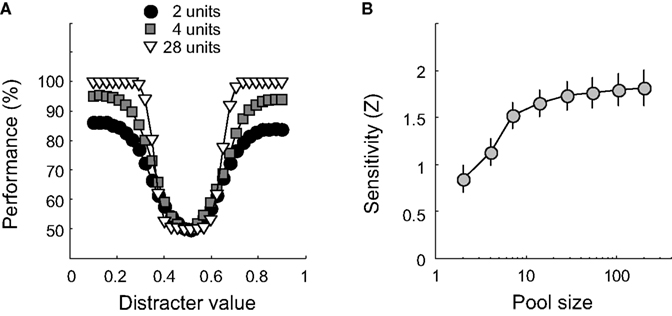
Figureà3. The effect of pool size on classification performance. (A)àClassification performance is plotted as a function of distracter value for three different pool sizes. Pool size is indicated by the figure legend. (B) Sensitivity as a function of pool size on semi-logarithmic coordinates. Error bars indicateà±Ã 1 SD.
Experiment I: The Role of the Selectivity for a Relevant and Irrelevant Dimension
In this experiment, we expand the task and network tuning to two dimensions and study the effects of average tuning width (i.e. selectivity) for both dimensions. The network was trained to discriminate a 2-D signal stimulus from a 2-D distracter stimulus. As was the case in the introductory experiment, the signal stimulus remained constant throughout the whole training, while the distracter stimulus was randomly selected from a set of eight stimuli on each training run. The design is illustrated in Figure 4
A. The blue symbols refer to the set of distracters, the green symbol to the signal. It can be seen that only one of both stimulus-dimensions is informative for this task. In the reminder of this paper, we will refer to this dimension as the ‘relevant’ dimension and to the other dimension as the ‘irrelevant’ dimension. The RD may be thought off as signalling object identity, while the ID could for instance code for object location or size.
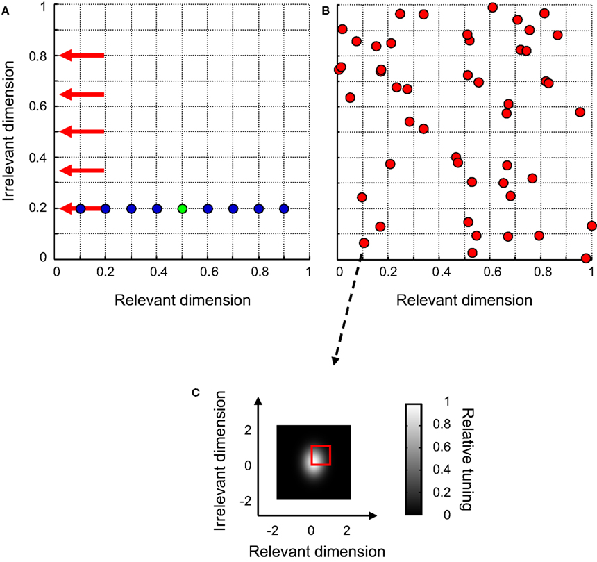
FigureÃÂ 4. The design of experiment I. (A) The network was trained to discriminate a 2-D signal (green symbol) from a 2-D distracter, randomly selected from a set of eight distracters (blue symbols) on each trial. Red arrows indicate the stimulus value on the ID in the five identification tests. (B)ÃÂ The distribution of peak-sensitivities of all units for one particular network. (C) The 2-D Gaussian-shaped tuning function of one network unit. The red square indicates the bivariate uniform distribution from which peak-sensitivities were randomly selected.
The networks trained to perform this task consisted of 49 units, tuned to both the RD and ID. Peak sensitivity of these units was randomly selected from a bivariate uniform distribution ranging between 0 and 1 on both dimensions. One example network is shown in Figure 4
B; red symbols indicate the peak-sensitivities of all network units. In this simulation, we investigate the role of the average 2-D Gaussian-shaped tuning width of the network units. Therefore, the average tuning width of the network units, expressed in σ, was varied between 0.125 and 1 for each dimension. The standard deviation of the tuning width was held constant atÃÂ 0.1. An example 2-D tuning function can be seen in Figure 4
C. Note that the peak sensitivity of this unit approximates (0, 0) – as can also be seen in Figure 4
B – and that the unit is more narrowly tuned for the RD than for the ID.
To measure identification ability, we made use of the task explained in the previous section, i.e. we tested how well the network managed to discriminate the signal from 30 previously unseen distracters that only differed on the relevant dimension. To test the invariance of the network’s signal representation, this identification test was run at five different stimulus-locations on the ID, indicated by the red arrows in Figure 4
A. One of these five identification tests was identical to the training circumstances (ID-testÃÂ =ÃÂ ID-trainÃÂ =ÃÂ 0.2). In the four other identification tests, the stimulus value on the ID differed from the training value (ID-testÃÂ =ÃÂ 0.35, 0.50, 0.65 and 0.80, respectively).
We first consider identification performance for the case where the ID value of the test stimuli equals the ID value of the training stimuli. Results, averaged over 30 networks, are shown in detail in the ‘identification’ column of Figure 5
for four different tuning width conditions (tuning width for the RD and ID being narrow-narrow, narrow-broad, broad-narrow and broad-broad, respectively). Classification performance is plotted as a function of distracter value. The average tuning width of the network units is illustrated by the 2-D tuning functions shown in the left panels of Figure 5
. The performance functions show that identification ability in circumstances that match the training situation (same ID value) benefits from narrow tuning on the RD. Further, identification may be slightly better if tuning on the ID is broad. This effect is clearer in Figure 6
A, which summarizes results of all tuning width conditions. Identification is expressed in sensitivity (i.e. the Z-statistic introduced in the previous section) and plotted as a function of average tuning width on the RD and ID. Inspecting the rows of the colour matrix reveals a rapid change in colour, indicating the importance of tuning width on the RD for identification sensitivity. However, the columns show a mild but consistent change in colour as well, indicating that average tuning width on the ID partly determines sensitivity. This second result may be understood as being a consequence of the pool size effect shown in Figure 2
E. Networks with units that are (on average) narrowly tuned to the ID will have some units that are not sensitive to the training stimuli, due to their location on the ID. Consequently, these units will not contribute to the decision statistic used by the SVM. Broad tuning to the ID, on the other hand, yields more units sensitive to the training stimuli and thus effectively larger pool sizes used by the SVM. In sum, when only one dimension is relevant for the identification task and the test situation matches the training situation, best performance is reached on this identification task when units are narrowly tuned to the RD and ‘ignore’ the ID.
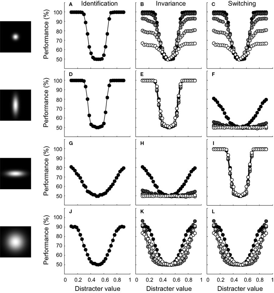
FigureÃÂ 5. Results of experiment I for four network-types. The leftward panels illustrate the average bivariate tuning functions of the network units. Conventions are identical to those of Figure 4
C. Identification. Classification performance is plotted as a function of distracter value on the RD. The ID value of all test stimuli was identical to the training situation. Invariance. Classification performance is plotted as a function of distracter value for five different ID values of the test stimuli. Symbol colour indicates the ID value (as symbols become lighter, the distance between ID-test and ID-train increases). Switching. Classification performance when the relevance of both dimensions is swapped.
We now wish to consider how performance of these networks generalizes to cases where the ID value of the test stimuli differs from the ID value of the training stimuli. Results, averaged over 30 networks, are shown in detail in the ‘invariance’ column of Figure 5
for the four tuning width conditions. Classification performance is plotted as a function of distracter value for five different identification tests, indicated by colour (black symbols refer to the case where ID-testÃÂ =ÃÂ ID-train; as symbol colour becomes lighter, the distance between ID-test and ID-train increases). Perfect generalization implies that network performance is not affected by the ID value of the test stimuli and would yield indistinguishable performance curves at all ID-test levels. This is the case for the network whose performance is shown in Figure 5
E. The units of this network are narrowly tuned to the RD, but broadly to the ID. For all other networks shown, however, identification performance suffers from the change in ID-test value relative to ID-train.
A more general summary of these results is shown in Figure 6
B. To express invariance in a single number, the ratio of the sensitivity at the most remote ID-test value and the sensitivity at ID-train was computed. This statistic thus expresses the proportion of identification sensitivity in the training situation preserved in the most extreme test situation. We shall refer to this statistic as the ‘invariance ratio’ – note that this relative performance measure is only meaningful when identification sensitivity in the training situation is reasonably high. In Figure 6
B, the invariance ratio is plotted as a function of average tuning width on the RD and ID. As was the case for the identification sensitivity shown in Figure 6
A, best invariance is found for networks whose units are narrowly tuned to the RD and ignore the ID. Similarly, invariance is worst for networks whose units are sensitive to the ID, but insensitive to theÃÂ RD. An important difference between identification and invariance performance, however, can be seen in the upward diagonal of the matrix, showing results for networks having a similar average selectivity for the RD and ID. In Figure 6
A, sensitivity decreases along this diagonal. In Figure 6
B, the invariance ratio increases along this diagonal. This suggests the existence of a trade-off between identification and invariance, a point that will be further clarified in the discussion.
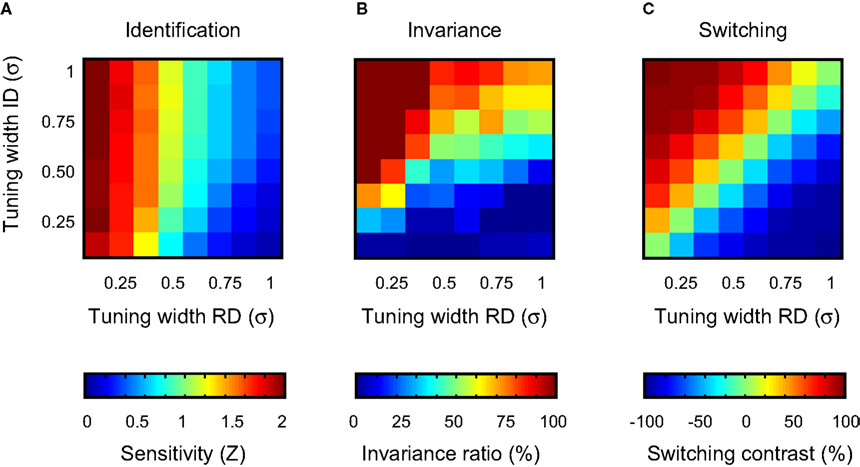
FigureÃÂ 6. Summary of the results of experiment I. (A) Identification sensitivity as a function of average unit tuning width on the RD and ID. Each cell summarizes results of one network-type. (B) The invariance ratio as a function of average unit tuning width on the RD and ID. (C) Switching contrast as a function of average unit tuning width on the RDÃÂ and ID.
A final issue we wish to address here is how network performance changes when RD and IDs are switched and the SVM is trained anew. We did not run a new simulation, but estimated this performance by swapping the network-tuning labels ‘RD’ and ‘ID’. For networks that have identical average tuning width for the RD and ID, performance estimates will thus also be identical. Results, averaged over 30 networks, are shown in detail in the ‘switching’ column of Figure 5
for the four tuning width conditions. Classification performance is again plotted as a function of distracter value for five different identification tests, indicated by colour (black symbols refer to the case where ID-testÃÂ =ÃÂ ID-train; as symbol colour becomes lighter, the distance between ID-test and ID-train increases). Perfect switching implies that network performance is not affected by the RD- or ID-label and thus that the ‘switching’ performance curves are indistinguishable from the ‘invariance’ performance curves. By definition, this is the case for the networks whose units have, on average, identical tuning width to the RD and ID (compare Figures 5
B,C, for instance). For networks whose units are differently selective to both dimensions, however, switching the relevance of both dimensions hurts or improves performance depending on which dimension was associated with most selectivity.
The switching results are summarized in Figure 6
C. To express switching performance in a single number, we first computed the general sensitivity averaged over all RD- and ID-test values for both the original and switched task (yielding Zor and Zsw, respectively). Then, the ratio of the difference of both sensitivities to the sum of both sensitivities was computed [i.e. (ZorÃÂ −ÃÂ Zsw)/(ZorÃÂ +ÃÂ Zsw)]. This statistic thus expresses the proportion of improvement in general sensitivity when the relevance of both dimensions is switched and varies between −1 and 1. We shall refer to this statistic as the ‘switching contrast’. Negative values indicate that general sensitivity benefits from the switch, positive that general sensitivity is hurt by the switch. The most intriguing aspect of Figure 6
C is that switching contrast is nearly constant when moving right/upwards. This is trivial for the upward diagonal (same data used for computing Zor and Zsw), but not for the other right/upward lines. This observation indicates that the proportion of change in general sensitivity upon relevance-switching is not determined by the absolute tuning width to either dimension, but solely by the difference in average tuning width for both dimensions.
Experiment II: The Role of Orthogonal or Independent Tuning
In this experiment, we introduce dependency of tuning and study the effects of mean dependence and variation in dependence. To clarify the effect of dependent tuning, some example 2-D tuning functions are shown in Figure 7
. Figure 7
A shows the average 2-D unit tuning function for the network under consideration. Note that selectivity for both dimensions is on average identical, broad, and independent. In the experiments discussed so far, tuning to both dimensions was always independent for all networks and each unit. In this example, the average dependence of the network units still equals 0, but some variation or scatter in the dependency of tuning was introduced (the correlation-distribution is depicted by the full black line in Figure 7
B). The effect of this scatter on the unit tuning functions is shown in Figure 7
C: most receptive fields are no longer horizontally or vertically orientated. This implies that the tuning for one dimension depends on the stimulus value on the other dimension. Consequently, the individual units have no invariant stimulus representations.
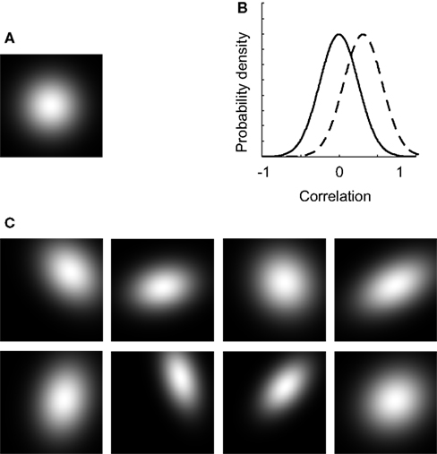
FigureÃÂ 7. The effect of dependent tuning. (A) The average 2-D unit tuning function for a particular network. (B) The correlation-distributions used in experiment II. (C) Some example unit tuning functions corresponding to the average tuning width shown in panel (A) and the correlation-distribution depicted by the full line in panel (B).
We first address the question whether a scatter in dependence hurts invariance at the level of the network representation when the average dependence equals 0. To this end, we replicated experimentÃÂ I for four different tuning width conditions (narrow-narrow, narrow-broad, broad-narrow and broad-broad, respectively). Results for networks with and without scatter in dependence are shown in Figure 8
(for the scatter condition, we used the correlation-distribution depicted by the full black line in Figure 7
B). At first sight, these performance functions reveal no strong effect of the introduced scatter in dependence. This conclusion is supported by the fact that the invariance ratios are hardly different from the ‘no scatter’ condition (i.e. in the order of Figure 8
: 13, 100, 3 and 47% for the ‘no scatter’ condition and 7, 100, 4 and 44% for the scatter condition, respectively). The only type of network with a convincing effect is the one of Figure 8
B, which is a network with narrow-narrow units, resulting in good identification performance and poor invariance. Nevertheless, also here the effect of a scatter in dependence is small. The main finding is thus that for networks that show no systematic dependence, invariance is mostly determined by the average tuning width for both dimensions. These networks thus manage to average out the scatter of dependence at the level of single units.
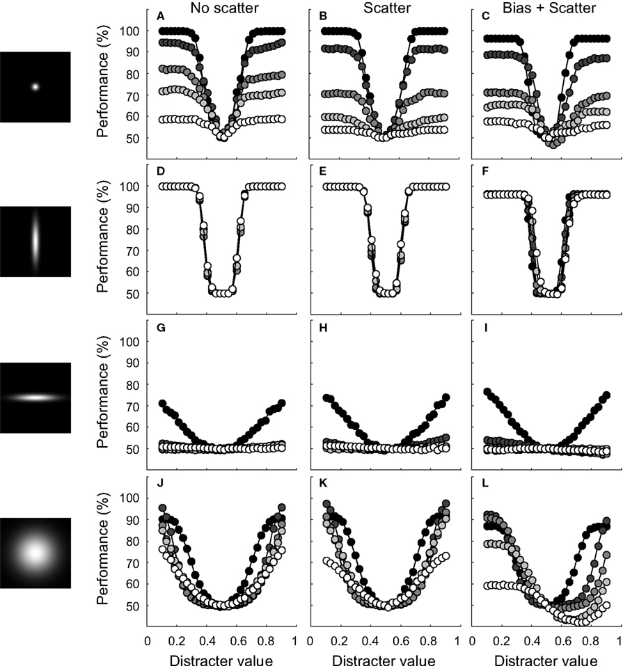
FigureÃÂ 8. Results of experiment II. The leftward panels illustrate the RD and ID selectivity of the average bivariate tuning functions of the network units. Conventions are identical to those of Figure 4
C. No scatter. Classification performance is plotted as a function of distracter value for five different ID values of the test stimuli. Conventions are identical to Figure 5
. For these networks, unit tuning functions were not correlated. Scatter. For these networks, average dependence was equal to 0. There was some variation in the dependence of the unit tuning functions, however, BiasÃÂ +ÃÂ scatter. For these networks, average dependence was equal to 0.3. There was also some variation in the correlation of the unit tuning functions.
How about networks that have an average dependence different from 0? Results for the same four tuning width conditions are shown in Figure 8
, under the heading ‘biasÃÂ +ÃÂ scatter’. This time, we used the correlation-distribution depicted by the dotted black line in Figure 7
B (the average correlation equals 0.3, the standard deviation of the correlation 0.25). The effects of an average dependence different from 0 – while present in all panels – are clearest in Figure 8
L. First, identification performance may now drop below guess rate. Second, results differ for distracters that have a lower value than the signal and distracters that have a higher value. For the former, performance in the vicinity of the signal has improved and is only slightly impaired at further distances. For distracters that have a higher value than the signal, on the other hand, performance is severely impaired. In general, the invariance ratio has lowered relative to the ‘no scatter’ conditions (i.e. in the order of Figure 8
: 13, 100, 3 and 47% for the ‘no scatter’ condition and 13, 99, −5 and 8% for the ‘biasÃÂ +ÃÂ scatter’ condition, respectively). Networks that have a systematic dependence in tuning thus show less invariance and asymmetric effects when tested for invariance in an identification test. The loss in invariance depends on the strength of the dependence, as is shown in Figure 9
. Here the invariance ratio for the ‘broad-broad’ network of Figure 8
is plotted as a function of average dependence (the standard deviation in correlation was always equal to 0.25). It is clear that the invariance ratio goes down when the average dependence goes up beyond 0.1.
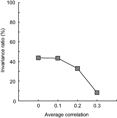
FigureÃÂ 9. Correlated neural noise in experiment III. The invariance ratio for the ‘broad-broad’ network of Figure 8
is plotted as a function of average dependence of the unit tuning functions (the standard deviation in correlation was always equal to 0.25).
Experiment III: Pool Size, Correlated Noise and Invariance
In this final simulation, we studied the effect of pool size and correlated noise on invariance. Single-unit recordings throughout the visual cortex, including ITC, have demonstrated that the responses of different cortical neurons in discrimination tasks are typically weakly correlated (Gawne and Richmond, 1993
; Golledge et al., 2003
; Shadlen et al., 1996
; Zohary et al., 1994
). Because correlated noise limits the encoding capacity of a pool of neurons and the strength of this limitation depends on pool size (Zohary et al., 1994
), weakly correlated noise is an important factor to consider when studying effects of pool size.
We replicated experiment I with networks that were equally sensitive to both dimensions and relatively broadly tuned (i.e. on average, σà=à0.5 for the RD and ID, with a standard deviation ofà0.1). We compare results for networks with no inter-unit correlations and networks whose unit responses are weakly correlated (the average inter-unit correlation being equal to 0.15). To see the effect of this correlation on unit responses, consider Figure 10
. In Figures 10
A,B, responses of one unit to 100 stimulus presentations are plotted as a function of the responses of another unit to the same stimuli. The neurons of Figure 10
A share no noise, while the responses of those shown in Figure 10
B are weakly correlated. The effects of such correlation at the level of a whole network can be seen in Figure 11
. Classification performance is plotted as a function of disctrater value for three different pool sizes, as indicated by the figure legend. To estimate these numbers, more repetitions were used for smaller networks than for larger networks. First, consider Figures 11
A,B, which show results at ID-train without (Figure 11
A) and with (Figure 11
B) correlated noise. Both figures cleary reveal a pool size effect, consistent with our findings for the simple identification experiment shown in Figure 3
, i.e. identification performance increases with pool size (up to a certain critical number of units, see Figure 3
B). Further, for the three pool sizes shown, weakly correlated noise slightly impairs identification sensitivity at ID-train. This, of course, is the equivalent of the well-known encoding-limitation effect of correlated noise for our identification experiment.
FigureÃÂ 10. The effect of pool size and correlated noise on classification performance in experiment III. (A) Responses of one unit to 100 stimulus presentations are plotted as a function of the responses of another unit to the same stimuli. These neurons share no noise. (B) Same as in panel (A) for units that share weakly correlated noise.
Figures 11
C,D show classification performance at the most remote ID-test value for the same pool sizes. In line with our earlier results, identification performance suffers from the change in ID-test value relative to ID-train (Figure 6
B reveals that the invariance ratio was estimated to be approximately 25% for similarly tuned networks consisting of 49 units). Intriguingly, however, comparison of the white and grey symbols in Figures 11
C,D shows a rather surprising pool size effect: The white symbols lay below the grey symbols, indicating that the smaller network outperforms the larger network. Thus, both without (Figure 11
C) and with (Figure 11
D) correlated noise included, a 25-units network is more tolerant for changes in the ID-test value than a 100-units network. A summary and extension of these results is shown in Figure 12
. Identification sensitivity is plotted as a function of pool size for both correlation conditions in the two different ID-test conditions on double logarithmic coordinates (circles refer to the sensitivity at ID-train, squares to the sensitivity at the most remote ID-test value; white symbols refer to networks with no inter-unit correlation; grey symbols to networks with correlated noise).
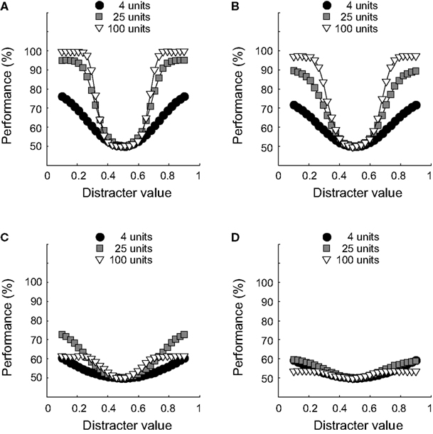
FigureÃÂ 11. The effect of pool size and correlated noise on classification performance. (A) Classification performance at ID-train is plotted as a function of distracter value for three different pool sizes (as indicated by the figure legend). Results in (A) are from networks without correlated noise. (B) Same as in (A) for networks with correlated noise. (C) Classification performance at the most remote ID-test location, results are from networks without correlated noise. (D) Same as in (C) for networks with correlated noise.
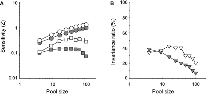
FigureÃÂ 12. Results of experiment III. (A) Identification sensitivity is plotted as a function of pool size for both correlated noise conditions in the two different ID-test conditions on double logarithmic coordinates (circles refer to the sensitivity at ID-train, squares to the sensitivity at the most remote ID-test value; white symbols refer to networks with no inter-unit correlation; grey symbols to networks with correlated noise). (B) The invariance ratio is plotted as a function of pool size for both correlated noise conditions (white symbols refer to networks with no inter-unit correlation; grey symbols to networks with correlated noise).
In Figure 12
A, the grey circles lie below the white circles. This indicates that weakly correlated noise lowers identification sensitivity at ID-train for all pool sizes. Intriguingly, comparison of the white and grey squares reveals that correlated noise hurts identification sensitivity even more at the most remote ID-test value. Correlated noise thus impairs invariance. This can also be seen in Figure 12
B. The invariance ratio is plotted as a function of pool size for both correlation conditions (white symbols refer to networks with no inter-unit correlation; grey symbols to networks with correlated noise). Even without correlated noise invariance tends to go down with increased pool size, but this phenomenon becomes stronger with correlated noise. Thus, for this network, increased pool size and correlated noise impair invariant identification behaviour.
The invariance ratio compares sensitivity at two different ID values. It can go down because performance at the trained ID value increases more rapidly than performance at the most extreme untrained ID value, while there is still an improved performance at this untrained ID value with larger pool sizes. However, we clearly see that performance at the most extreme untrained ID value can go down with larger pool sizes, which is really surprising. Identification sensitivity at the most remote ID-test value initially improves with pool size but from a certain number of units on decreases as a function of pool size for both correlated noise conditions (see Figure 12
A). Invariance does thus not benefit from larger pool sizes (see Figure 12
B). To the contrary: invariance is approximately 0 for fairly large pool sizes.
This counter-intuitive finding can be understood from what is learned by SVMs. In small networks, relatively little information about the stimulus is present. Each unit represents some unique information and is thus used by the SVM in determining the decision statistic. This is also the case for units that are not ideally tuned to the training stimuli due to their ID selectivity. When identification performance is tested at a different ID location, the most informative units of the training stage might suddenly mainly contribute noise to the decision statistic. In contrast, the units that were not optimal during training due to their ID selectivity may now be valuable. This leads to an approximation of invariant behaviour. In large networks, the SVM is offered the luxury to compute its decision statistic almost entirely based on response patterns (vectors) that put a strong emphasis on units which are optimally tuned to the training stimuli. Due to the large amount of information present in the network, the SVM can ignore the units that are not ideally tuned to the training stimuli. Consequently, identification performance under training circumstances will be better when compared to smaller networks, as is also borne out by our data. The price to pay, however, is that the robustness of the network to unexpected changes in the test situation has decreased significantly. In this regard, these results are yet another manifestion of the fundamental trade-off between selectivity and tolerance existing at population level.
We investigated the relationship between single-unit tuning properties and population-level read-out performance in terms of identification performance, invariance, and switching. The results indicate how difficult it is to find a neural code that allows good performance according to all three of these measures. Most importantly, the read-out of a population of non-invariant single units is non-invariant itself.
Effects of Bivariate Tuning Properties on Identification and Invariance
We started with a simple network with units tuned along one dimension. This experiment illustrated how even a network with a fairly small number of units can decode the value of a target stimulus. This performance was obtained even though the identification problem is essentially non-linear: the target is surrounded by distracters at both sides of the stimulus dimension.
Here we are mostly interested in performance when there is at least one irrelevant stimulus dimension. Good identification ánd good invariance was obtained when individual units in a population were very selective for the RD and very broadly tuned for the ID. In this case the independence of tuning for the two dimensions did not matter. This finding follows the intuition that has lead to the proposal of very abstract object recognition models: invariant behaviour calls for invariance in tuning. However, it already became clear from the Introduction that the brain has not implemented this solution. There are at least two possible reasons for this. First, a strong difference in tuning for the two dimensions leads to inferior switching when the relevance of the dimensions would change or reverse. It can be argued that the distinction between RD and IDs, and the stability of this distinction, is not so clear-cut in natural vision. For example, stimulus position, which seems to be irrelevant for object recognition, might be helpful to represent the relative position of parts in multi-part objects (Edelman and Intrator, 2000
). Thus it might not be optimal to reduce the selectivity for such dimensions to 0.
Second, the primate visual system might not be able to create single neurons with the desired properties of high selectivity for the RD and low selectivity for the ID. Indeed, Zoccolan et al. (2007)
observed a trade-off between object selectivity and tolerance at the single-neuron level. ITC neurons with higher object selectivity tended to be more influenced by image transformations such as changes in position or size. Thus, even if the distinction between RD and IDs might be clear-cut from a conceptual point of view, the practical implementation of this distinction into neurons that are only sensitive to changes in these RDs might be impossible. Whatever the reason why ITC neurons do not achieve the tuning characteristics that optimize both identification and invariance, the conclusion is that they do not.
So it is most relevant to look at our simulations with a range of other less extreme tuning widths for RD and ID. In general, the findings followed naturally from the aforementioned extreme case. High selectivity on the RD is beneficial for identification, while selectivity on the ID had little effect on identification (with a small beneficial effect of less ID selectivity). Low selectivity on the ID is beneficial for invariance. However, in addition we noted an interesting trade-off between identification and invariance when RD and ID selectivity was similar: High selectivity on both RD and ID is associated with good identification and poor invariance, while low selectivity on both RD and ID is associated with poor identification and good invariance. Note that this trade-off determines the performance of reading out a neural population, while the trade-off observed by Zoccolan and colleagues was characterized at the single-neuron level. The single-neuron trade-off prevents the system from having very different selectivity for RD and ID, and this causes the system to be in a situation where the read-out of the responses is subjected to a trade-off between identification and invariance. From these trade-offs, we would predict that ITC neurons would not be extremely selective for objects, as this would hurt invariance both at the single-neuron level (as shown by Zoccolan and colleagues) and at the population level (as shown here).
Correlations in the bivariate tuning of neurons had two sorts of effects. A first effect was obtained in cases where the average correlation deviated from 0. In that case, the invariance performance was affected very strongly and in an asymmetric way. However, high deviations in the average correlation are somewhat artificial. If it would be encountered in actual data, then it would be a strong indication that the way dimensions were defined by the experimenter does not fit with the dimensions that define single-unit tuning or behaviour (see Ashby and Townsend, 1986
). In most situations, we expect to see a scatter of the correlation around a mean correlation that is closer to 0. The effect of this scatter in the correlation was very small overall. However, it interacted with tuning width along RD and ID in such a way that the strongest effect of scatter in correlation was noted in a case with low invariance. The same was true for cases in which the average correlation differed from 0. In those situations, more scatter in correlation decreases invariance. Thus, an increase in the independence of tuning for RD and ID at the single-neuron level is one way to increase invariance.
These findings suggest that a linear classifier looking at the output of a neural population averages out the possible scatter in tuning properties to a certain degree. Including more neurons also improves identification performance under training circumstances. Nevertheless, contrary to what one might expect intuitively, population-level classification was not more invariant to changes in the ID. We have even observed the opposite: stronger effects of the value on the ID with a larger population size. Thus, if neurons on average show clear sensitivity for a particular image transformation, then population-level classification will also be sensitive to this image transformation, and sometimes even more so. From that perspective average single-neuron selectivity might provide an upper-bound of the degree of invariance possible in a neural network.
Implications and Limitations
The merit of this study is that we provide an explicit test for the hypothesis that a linear read-out mechanism of a pool of units resembling ITC neurons may achieve invariant performance in an identification task. Further, this work draws an explicit connection between the recent work on multivariate analyses of patterns of selectivity across neurons and fMRI voxels and older work on multidimensional tuning properties of single neurons. Without this explicit connection, we are left wondering how the two sets of studies connect, and whether a particular outcome of a multivariate analysis is consistent with previously published single-unit data. Papers in the literature have not studied identification and invariance at both the single-neuron and population level, but nevertheless it is possible to derive that empirical findings are generally in line with our conclusions. Importantly, Hung et al. (2005)
suggested that SVMs trained on data from objects presented at one position or scale are able to perform very well with data obtained at another position or scale, with only a small drop in performance (from 76 to 70%). We noted in the Introduction that this finding might suggest a discrepancy between network-level and single-unit invariance as empirical studies have revealed small receptive fields in ITC (DiCarlo and Maunsell, 2003
; Op de Beeck and Vogels, 2000
). However, while the latter studies revealed the existence of small receptive fields in ITC and a large scatter of receptive field size, the average receptive field was large enough to encompass the fairly small 4 visual degrees variation that was included to train and test the classifiers by Hung et al. (2005)
. Thus, the invariance of population-level classifier performance did not exceed expectations based on single-neuron tuning curves. Furthermore, the approximation of invariance by Hung etÃÂ al. might be an over-estimation as they studied neurons whose responses were not measures simultaneously. So their neural populations included no correlated noise. Our results reveal that invariance might be lower with correlated noise.
Our simulations do not exhaust all possible options of network characteristics. First, we used Gaussian tuning curves. This is the most common distribution to fit the tuning of neurons (e.g. McAdams and Maunsell, 1999
; Op de Beeck and Vogels, 2000
; Schoups et al., 2001
) and in modelling work (e.g. Poggio and Edelman, 1990
; Pouget et al., 2000
). Furthermore, it is also the best distribution to take as the general ‘default’ as it is a maximum entropy distribution. Nevertheless, other distributions can be considered, some ‘bell-curved’ like the Gaussian distribution, other more monotonic. Which tuning function is the optimal depends on many factors, including the characteristics of the neural noise, read-out constraints, and the mechanisms by which these tuning functions are generated (see e.g. Beck et al., 2007
; Ben-Yishai et al., 1995
; Salinas, 2006
; Series et al., 2004
). Thus, while we targeted the most general case by using Gaussian functions, it is important to consider that some of the observed effects might differ with other tuning functions.
Second, we have only shortly looked at effects of correlated noise and population size, and much more can be done. Note that correlated noise is a totally different aspect of a neural code than the correlation/independence in the tuning along multiple dimensions. While the latter characterizes the multidimensional tuning of a single neuron, the former refers to the dependencies in the noise distribution between neurons. Such correlated noise is known to affect how performance rises with increases in population size (Shadlen and Newsome, 1998
; Zohary et al., 1994
), and a similar effect was observed in our simulations. We were surprised to note that the presence of correlated noise does not only limit identification performance but also invariance, and we have checked that this phenomenon occurs for a wider range of parameter combinations than the ones reported here. Nevertheless, there are many aspects of correlated noise that we did not study, such as what happens when the degree of correlated noise is different for units with high and low selectivity, and effects of the exact circuit mechanisms that are used to achieve the high selectivity (Pouget et al., 1999
).
Third, we have selected one type of classifier, linear SVMs, to assess read-out performance. This selection was chosen based on its prevalence in recent neurophysiological and neuroimaging studies. Many other multivariate measures can be taken. However, an important restriction is that all these measures should combine the output of the units in a linear way. Non-linear mechanisms would be more powerful and flexible, but they do no longer tell us how well a next layer of neurons would be able to read-out the information in a neural representation (DiCarlo and Cox, 2007
; Kamitani and Tong, 2005
). Nevertheless, read-out processes in the real brain might be more powerful than implemented here. For example, we assumed read-out mechanisms that look at the full pattern of selectivity. Instead, separate classifiers could be built that include special sub-classes of neurons, selected based on prior experience. It has been previously observed that real neurons are very diverse in their tuning properties (e.g. Op de Beeck et al., 2008b
), and this element was also included in the present investigation. However, the simulations did not include any a priori labelling of neurons as being ‘good’ or ‘bad’ for the task at hand. The real brain is not a tabula rasa in which a new task is learned without reference to any previous task, and shortcuts based on previously established learning and wiring might increase the efficiency and speed of reading out object representations in an invariant manner.
In sum, our study was motivated by the observation in the literature that object-selective neurons are also selective to a certain degree of image transformations such as position and size. The average neuron does not attain the ideal of high object selectivity combined with high invariance for such transformations, and there is even a trade-off that makes it very unlikely to find any ideal neurons. We show that also measures that look at the pattern of response across populations of such non-ideal neurons show non-ideal performance: good identification performance and invariance are not found together, and a trade-off between the two is also found at the population level. The situation was even worse when these non-ideal neurons displayed correlated tuning for RD and ID. We conclude that a network composed of neurons that do not individually show good object selectivity and good invariance will as a network also be unable to attain good object selectivity combined with good invariance.
Finally, we should note that the limited invariance is related to a situation in which the classifier or decoder only encounters one value of the ID during training. The same classifier would easily attain invariant performance if it would be trained on a wider range of values on the ID. Here we can refer to the literature on the recognition of objects across viewpoints. It was shown previously that it is possible to attain view-invariant performance with a network composed of orientation-selective units if the neural network is trained on three very different views (Logothetis et al., 1994
; Poggio and Edelman, 1990
). The exact number of training values on an ID that are needed to achieve invariant performance will again depend on the neural selectivity for that dimension.
Based on these data, behavioral evidence of invariant recognition suggests that either the visual system has encountered enough variability on IDs, or that the visual system has implemented read-out processes that are more powerful to serve the goal of invariance than the linear classifier considered here. Nevertheless, in the case of ‘overlearned’ visual stimuli like human faces or letters, there are behavioral analogues to our simulated results. While we are very sensitive for small differences between faces and experts in recognizing letters, behavioral performance decreases severely when faces or a text are inverted or presented at an unusual size (McKone, 2009
; Pelli, 1999
; Robbins and McKone, 2003
). While this is no evidence that a similar mechanism as the one we simulated underlies these effects, it is interesting to note that for certain special classes of stimuli, our visual system is highly selective, but only mildly tolerant at behavioral level. Thus, a population read-out of only moderately invariant single neurons does not automatically result in invariant performance.
The authors declare that the research was conducted in the absence of any commercial or financial relationships that could be construed as a potential conflict of interest.
Thanks to C. Baker and G. Kayaert for their valuable comments on a previous version of the manuscript, and to J. Wagemans for his continuous support. This research was supported by a predoctoral (R.L.T.G.) and postdoctoral (H.P.O.) fellowship from the Fund for Scientific Research (FWO) of Flanders, the K.U.Leuven research council (project CREA/07/004), and the Human Frontier Science Program (CDA 0040/2008).