 Eric O'Shaughnessy
 Galen Barbose
 Alexandra Grayson
 Isa Ferrall-Wolf
 Deborah Sunter4
94% of researchers rate our articles as excellent or good
Learn more about the work of our research integrity team to safeguard the quality of each article we publish.
Find out more
ORIGINAL RESEARCH article
Front. Sustain. Energy Policy, 16 November 2023
Sec. Energy and Society
Volume 2 - 2023 | https://doi.org/10.3389/fsuep.2023.1203517
Household decisions to adopt rooftop solar photovoltaics are partly driven by social influence. Previous research on solar adoption influence has focused on influence among residential peers. Here, we expand the framework of solar adoption influence by exploring the influence of non-residential installations on residential adoption decisions. We use staggered differences-in-differences to estimate non-residential influence effects using a large data sample of residential adoptions. We also critically evaluate prevailing frameworks for solar adoption influence. We find that non-residential installations are associated with accelerated residential adoption rates, on the order of 0.4 additional residential adoptions per quarter per non-residential installation. We show that non-residential systems exert a continuous, long-term influence on residential adoption decisions. We explore separate results and influence mechanisms for solar installed on commercial buildings, government buildings, and houses of worship. The results suggest that non-residential solar adopters could serve as partners in policies to “seed” residential adoption in underserved communities.
More than 3 million households had adopted rooftop solar photovoltaics (PV) in the United States by the end of 2022 (Davis et al., 2022). Every rooftop PV system reflects the outcome of an idiosyncratic individual or household adoption decision. A growing literature has emerged to explore what explains rooftop PV adoption decisions, such as financial incentives, environmental motivations, and customer interest in novel technologies (Sintov and Schultz, 2015; Alipour et al., 2020; Schulte et al., 2022). Within that literature are several studies showing that individual rooftop PV adoption decisions are partly driven by the adoption decisions of other individuals (Bollinger and Gillingham, 2012; Graziano and Gillingham, 2015; Moezzi et al., 2017; Palm, 2017; Mundaca and Samahita, 2020; Balta-Ozkan et al., 2021; Bollinger et al., 2022). The impacts of previous adoptions on subsequent adoption decisions are evident in the physical clustering of PV systems and statistical associations between the timing of PV installations and adoption decisions (Bollinger and Gillingham, 2012).
The relationship between past and subsequent PV adoptions has been characterized as a form of social influence (Axsen and Kurani, 2012; Xiong et al., 2016; Baranzini et al., 2017; Wolske et al., 2020). The term “influence” has been used in PV adoption research in a broad sense. Rooftop PV adoption decisions may be directly affected by active social interactions, such as with neighbors who have already adopted (Sigrin et al., 2017). The literature also suggests a role for more passive influence mechanisms, such as an individual being primed to adopt PV after seeing panels installed on another home (Graziano and Gillingham, 2015; Baranzini et al., 2017; Bollinger et al., 2022). Some have characterized PV influence as a form of social contagion (Axsen and Kurani, 2012; Xiong et al., 2016; Baranzini et al., 2017; Wolske et al., 2020), implying a process through which individuals are unconsciously influenced by the diffusion of PV systems. Here, we use the term “PV influence” to broadly describe any impacts of previous PV adoption decisions on subsequent adoption decisions.
PV influence research has mostly focused on influence in residential adoptions, but influence is not necessarily confined within residential peer groups (Baranzini et al., 2017). Rooftop or ground-mounted PV systems installed at non-residential establishments could likewise influence residential adoption decisions.1 Non-residential PV influence is of interest for several reasons. First, non-residential PV influence may quantitatively vary from the effects of residential installations. For instance, non-residential systems may generate more influence due the larger size of non-residential relative to residential systems. Alternatively, large ground-mounted non-residential systems could generate some degree of public resistance like that associated with larger utility-scale systems (Carlisle et al., 2016), which could decelerate residential PV adoption. Second, non-residential actors may be able to use unique channels of influence to promote PV adoption. For instance, houses of worship directly engage with and can influence the behavior of their congregations (Van Cappellen et al., 2016) and can serve as conduits for public policy implementation (Evans and Hudson, 2014; Flórez et al., 2017). Third, installers or policymakers could leverage non-residential influence by installing “seed” systems, following the rationale that installing a seed system promotes subsequent adoptions (Zhang et al., 2016; Sigrin et al., 2022). Installers could use seeding to promote business in new markets, and policymakers could use seeding to promote deployment in underserved communities, an increasingly common policy objective (Carley et al., 2021). Seeding policies could be more effectively designed if seeding interventions are targeted at building types that maximize influence.
In this study, we explore the impacts of non-residential installations on residential adoption decisions in the United States. We explore the hypothesis that non-residential PV installations influence residential PV adoption rates. We also explore how non-residential PV influence compares in magnitude to residential PV influence. We begin with a background discussion of how our theoretical and empirical models vary from PV influence research to date.
Previous rooftop PV influence studies have framed their models as quantifying peer effects, meaning the impacts of previous adoptions on subsequent adoptions stemming from interpersonal influence among peers—primarily meaning residential neighbors. Researchers have generally estimated peer effects by modeling PV adoption rates as functions of PV installation rates (Bollinger and Gillingham, 2012; Richter, 2013; Graziano and Gillingham, 2015; Baranzini et al., 2017; Bollinger et al., 2022). The logic is that influence begins after systems are installed and become visible. These models mostly share four characteristics. First, the models exploit the temporal lags between adoption decisions and system installations, two events that are typically separated by weeks or months. The lags between these two events allows researchers to identify the impacts of previous adoptions on subsequent adoptions. Second, PV peer effects are typically modeled within defined geographic areas, such as zip codes, such that influence is measured among near neighbors. Third, the models do not specify the mechanisms of influence. That is, estimated peer effects can reflect various influence mechanisms, such as active interactions between peers and passive influence from system visibility. Fourth, the measured effects are contemporaneous, meaning that the models estimate the impacts of installations on adoptions in the same time period.
Our approach largely builds on residential peer effect methodologies and shares the first three of the four characteristics outlined above. Still, our theoretical model and empirical specification deviate in important ways from previous work. In terms of the theoretical model, we discard any assumptions about the nature of PV influence and use the term influence effects to capture any impacts of previous adoptions on subsequent adoption decisions. Our definition does not imply a peer-to-peer basis nor do we make any assumptions about the social nature or mechanism (e.g., panel visibility) of the influence. We believe this terminology more accurately reflects what is being measured, not only in our results but in all PV peer effect models. To illustrate, suppose a PV contractor installs a PV system in a neighborhood and markets to that customer's neighbors. Peer effect models do not distinguish subsequent adoptions in this example that resulted from direct interactions among neighbors (i.e., peer influence) from those that resulted from broader social contagion such as the change in the installer's marketing patterns or simply the visibility of the original PV system. As a result, peer-effect models likely overstate the degree of true peer influence by measuring impacts unrelated to social interaction. Rather than attempt to isolate peer influence we simply accept that the estimates reflect a broader range of influence mechanisms.
A novel contribution of our empirical model is that we estimate the impacts of continuous, long-term influence, in contrast to prior peer effects models that estimate only contemporaneous impacts. That is, our model estimates influence effects under the assumption that a system installed in one quarter continues to influence residential adoptions in subsequent quarters. The notion of continuous influence is supported by the fact that certain PV influence mechanisms, namely system visibility, persist over time. Further, if an install influences an adoption in one quarter, that influenced residential install itself becomes a source of influence in subsequent quarters, such that influence may accumulate over time. Likewise, an install in one quarter can change market conditions in ways that affect residential adoptions in subsequent quarters, such as by inducing an installer to begin marketing in that area. Our approach estimates influence effects resulting from associations between a non-residential install and contemporaneous residential adoptions as well as long-term associations resulting from direct or indirect influence. For these reasons our results are not directly comparable with previous residential PV peer effect estimates.
As described above, we largely build on previous peer effect models by estimating the impacts of non-residential installations on residential adoptions. Like Bollinger and Gillingham (2012), we model influence at the zip code level. Section 3.1 describes our data sources, Section 3.2 describes our empirical model, and Section 3.3 notes several methodological limitations.
Our approach requires data on non-residential PV installation dates (physical installation) and residential PV adoption dates (adoption decision). We compiled non-residential installation dates from the Lawrence Berkeley Laboratory's Tracking the Sun (TTS) data set of PV system installations (Barbose et al., 2021). TTS includes records on over 80% of rooftop PV systems installed in the United States. About 3% of all TTS records are non-residential systems. Of those non-residential systems, about 77% are installed on building rooftops, while about 23% are ground-mounted on the premises of non-residential buildings. The TTS data include dates for when PV systems were interconnected to the grid. Data compiled by NREL (2023) suggest that PV installations typically occur around 25 days before interconnections, based on median installation timelines (average durations are 33 days with a standard deviation of 25 days). We therefore adjust the non-residential interconnection dates 25 days backward to create installation date proxies (Figure 1).
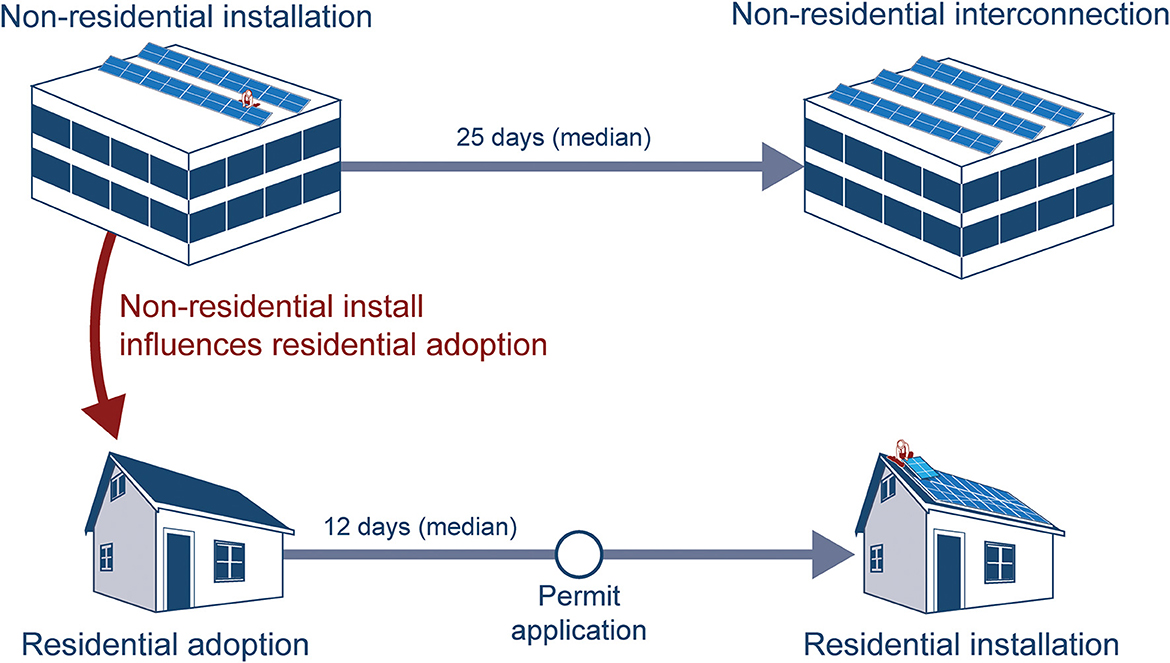
Figure 1. Schematic of PV influence identification strategy.
We estimate influence effects from 35,526 non-residential systems, comprising all non-residential building types that had adopted PV in any of the service territories covered by the TTS data set. To explore the robustness of the results across non-residential building types, we also implement separate models for systems installed on commercial buildings, government buildings, and schools using the TTS data. We were also interested in the potential influence of houses of worship, given previous research showing the effects of house-of-worship influence on the behavior of their congregations (Van Cappellen et al., 2016; Yale, 2022). We used data provided by Interfaith Power and Light2 and data from the Department of Homeland Security's (DHS) Homeland Infrastructure Foundational-Level Data matched to TTS addresses to identify houses of worship that had adopted rooftop PV. To confirm the DHS records accurately identify non-residential houses of worship, we used an address verification service procured from melissa.3 That service suggested that some DHS records were residential addresses. A spot check using Google Earth satellite images suggested that roughly half of DHS records coded as residential in fact referred to residential buildings. These records may refer to homes of individuals affiliated with houses of worship. Therefore, we restricted the combined data set to records identified as businesses by the Melissa Data identifier. A further spot check suggests that all records in that subsample are correctly identified as houses of worship. Using these sources, we built four separate samples of non-residential systems installed from 2010 to 2021 for commercial (N = 23,975), government (N = 3,989), schools (2,089), and house of worship (N = 1,329) installations. Note that the “all” non-residential category (N = 35,526) includes buildings in the subsamples that were not specifically identified (e.g., some schools may be simply coded as “non-residential”) and other building types not included in the four subsamples (e.g., secular non-profits, non-government public buildings). The four separate samples are roughly equally distributed across the 29 states tracked in the TTS data. Schools tend to have the largest systems, with a median capacity of around 83 kilowatts (kW), compared to 47 kW for government systems, 40 kW for commercial systems, and 33 kW for houses of worship.
Our source for residential PV adoption dates is a large set of residential PV adopter data compiled by BuildZoom, an online platform connecting customers with contractors. These data represent on-site residential systems—mostly rooftop—and do not reflect off-site residential solar options such as community solar. The final, cleaned set includes 1,449,189 records for residential PV adoptions from 2010 to 2021. The advantage of the BuildZoom data is that the set includes dates for when adopters applied for local permits. These permit application dates provide much closer proxies for adoption dates than the interconnection dates in TTS. Again, using NREL data on median timelines, we adjust the residential permit application dates 12 days backward from the permit application dates to create proxy adoption dates. However, the advantage of more precise dates in the BuildZoom data come with the tradeoff of smaller sample size. We analyze the larger TTS residential adoption sample as a robustness check in Section 4.2.
To motivate our approach, consider an ideal experiment to test the impacts of non-residential installations on residential adoption. A researcher in this ideal experiment would randomly install non-residential systems in a “treatment” group then compare how the number of adoptions—henceforward referred to as adoption levels—changes in the treatment group relative to a “control” group. Our approach follows this conceptual ideal. We use the standard terminology of treatment to refer to non-residential installations, the treatment group to refer to zip codes with non-residential installs, the control group to refer to zip codes without non-residential installs, and the treatment effect as the estimated impact of non-residential installs on residential adoptions in the same zip code.
Differences-in-differences (DiD) is a common method for replicating the ideal experiment described above in an empirical context. DiD models identify treatment effects based on the differences in temporal trends in the treatment and control group. The treatment group in our case comprises zip codes with at least one non-residential PV system installed after 2010 (we return to the rationale for ignoring 2010 non-residential installs further below). All zip codes with at least one residential PV adoption and no non-residential installs from 2010 to 2021 are candidates for the control groups. We use propensity score matching to determine which candidate zip codes are used as controls. Propensity score matching is a common approach for mitigating the impacts of confounding differences between treatment and control groups. The propensity score is an estimate of the probability that a unit is treated, in this case the probability that a zip code has a non-residential PV install. The approach estimates propensity scores based on factors that affect the outcome (in this case PV adoption levels, i.e., adoptions per quarter per zip code) and correlate with the treatment (in this case non-residential PV systems). We calculated propensity scores based on the factors described in Table 1 using the matchit package in R (Ho et al., 2011). We then used the propensity scores to construct control groups comprising equal numbers of zip codes as the treatment groups.
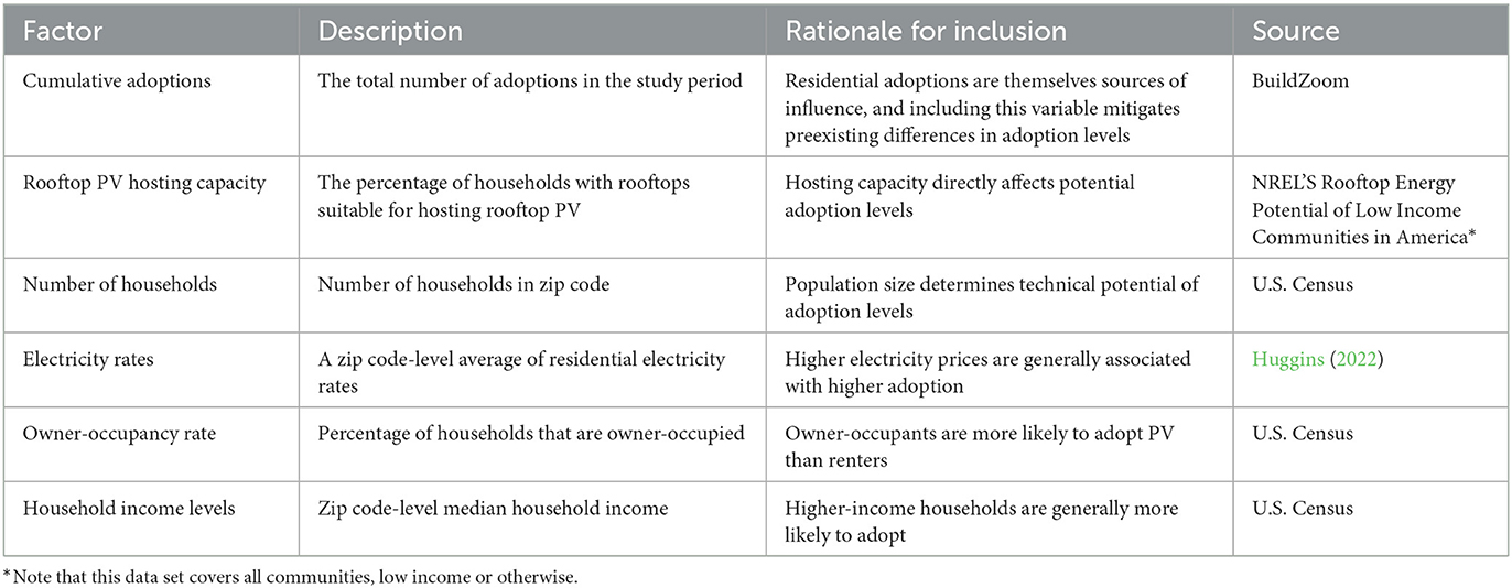
Table 1. Propensity score matching factors.
Using the propensity-matched treatment and control groups, we constructed a balanced panel data set at the quarter level (i.e., 4 blocks of 3-month increments in each year). The “treatment” occurs in the quarter in which a non-residential system is first installed. In standard DiD models the treatment occurs across the whole treatment sample at the same point in time. In this case the treatment occurs at different points in different zip codes throughout the study period, also known as a “staggered” treatment. We estimated staggered DiD using the group-time model developed by Callaway and Sant'Anna (2021). The group-time approach assigns each zip code into a group g based on the first quarter in which a non-residential system was installed (all control zip codes are in the same group). The approach estimates influence effects through the following model:
Where az∈g, q is the adoption level (i.e., number of adoptions) for zip code z in group g in quarter q,4 Gg is a group indicator variable, Qq is a quarter indicator variable, and Xzq is the vector of covariates used for the propensity score match (see Table 1) plus an additional control for the average value of state-level incentives in each quarter by state. The coefficient θgq estimates group- and time-variant differences in adoption rates, known as group-time effects. Group-time effects are the equivalent of the DiD estimator in a standard, non-staggered DiD model. For this reason, we excluded zip codes with non-residential installs in 2010 to ensure that DiD could be estimated with at least 4 pre-treatment periods. Conditioning on the control variables in Xzq ensures that other confounding factors do not explain deviations in parallel trends. Importantly, by including cumulative residential adoptions (the variable typically used to measure residential peer effects), we control for the confounding effects of residential PV influence. We add the state-level incentive value variable to control for changes in incentive levels over time and how those changes may affect residential demand, such as the introduction of new incentives in certain quarters and the decline in rebate values over time in some programs.5 The state-level incentive was estimated using incentive values reported to utilities and compiled in the TTS data set. The incentives reflect state or utility rebates, tax credits, or production-based ($/kWh) incentives provided throughout the study period. The incentive values do not reflect other clean energy policies such as local decarbonization targets or community solar programs.
The central question is whether group-time effects vary in post-treatment periods, i.e., for periods q > g. Our key metric to answer that question is the average treatment effect, which is provided by the group-level averages of the post-treatment group-time effects, i.e., . The hypothesis is that adoption levels are higher in the post-treatment quarters, such that . Following Callaway and Sant'Anna (2021) we present results for average treatment effects weighted by group sample size. As noted in Section 2, the estimated effects reflect the average of contemporaneous impacts and long-term influence in every quarter after non-residential systems have been installed.
Point identification of the average treatment effect requires the assumption of parallel trends in the treatment and control groups in a counterfactual scenario with no non-residential installations. The parallel trends assumption is untestable and often unrealistic in practice (Rambachan and Roth, 2022). Following Manski and Pepper (2018), we relax the point identification assumptions and partially identify non-residential influence effects. Partial identification is an approach that calculates a potential set of estimates containing the true value in lieu of calculating a single point estimate (Tamer, 2010). Formally, instead of attempting to identify the treatment effect using a single point estimate , we instead assume that the treatment effect belongs to a bounded set. The advantage of partial identification is that we can identify this set of estimates under weaker assumptions than those required for point identification. We bound the group-time effects based on estimated pre-trends for each group: . For each group we estimate a bounded group-time effect equal to . We then present an average bounded treatment effect weighted by group sample size. To summarize, we present results for two average treatment effects:
Where ATT is the unbounded average treatment effect, |ATT| is the bounded treatment effect, and wg is the weight for group g, the group sample size.
One key remaining concern is exogenous changes that drive spurious correlations between non-residential installations and residential adoptions at the zip code level. The most likely source of such correlations is exogenous changes in installer marketing patterns. That is, installers may install a non-residential system in a zip code at the same time they begin marketing to residential customers in that zip code. To control for this issue, we identify data subsamples where non-residential installs are theoretically less correlated with exogenous residential marketing patterns. We define “specialist” installers as those who install at least as many non-residential systems as residential systems. About 17% of installers in the TTS data sample are specialists by that definition. Specialist installers tend to operate at relatively small scales, such that specialists only account for about 0.7% of residential systems installed in the TTS sample. We construct alternative treatment and control groups following the same procedures described above limited to subsamples of non-residential systems installed by specialists. That is, we define treatment groups based on non-residential installs by specialist installers and estimate treatment effects based only on changes in residential adoption levels in the treated zip codes. The logic is that the movements of specialist, non-residential installers are less likely to correlate with exogenous changes in residential marketing patterns, thus mitigating that potential source of confounding correlation. This process largely eliminates positive pre-trends but substantially curbs sample size (see Table 2), significantly reducing the statistical power of the models. Still, by reducing the impacts of potentially confounding trends, we believe these subsamples yield more accurate estimates of non-residential influence effects. In the case of houses of worship, the specialist sample comprised just 70 house-of-worship installations. To avoid inferring from a small sample, we relaxed the specialist definition for house-of-worship installs to installers for whom non-residential systems account for at least 20% of sales.6
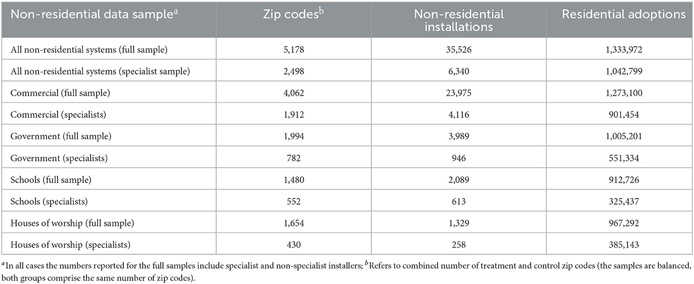
Table 2. Data samples.
We note two limitations of our analysis before proceeding to the results. First, the results across building types are not perfectly comparable given the substantial differences in sample sizes between the commercial, government, school, and house-of-worship samples. Further, around two-thirds of zip codes in the commercial treatment sample have more than one commercial system, compared to around one-third in the house-of-worship sample and about 10% in the case of the government sample. We present separate results for each building type primarily as a robustness check for the overall influence of non-residential systems. We discuss potential metrics to compare influence across building types in Section 3.1. Second, our use of DiD requires us to construct panel data based on discrete geographic units (zip codes). Influence effects are not necessarily confined to these arbitrary boundaries. Heterogeneous influence effects likely exist below the zip code level, as demonstrated by evidence that influence varies down to the street level based on panel visibility (Bollinger et al., 2022). Similarly, influence effects likely spill over beyond zip code boundaries. For instance, houses of worship may influence congregation members who live in zip codes surrounding the location of the PV system. The results should therefore be interpreted as proxies for influence effects based on the arbitrary boundaries provided by zip codes.
We present results in two parts, exploring our two research questions: whether non-residential installations influence residential adoption decisions, and how that influence compares to the effects of residential installs on residential adoption decisions. We begin by exploring the estimated non-residential influence effects in Section 4.1. In that section, we show how the models generally support the hypothesis that non-residential installations drive an increase in residential adoption rates. The magnitude and significance of that influence correlates with underlying sample size, such that smaller samples (e.g., houses of worship, schools) generally yield weaker results. We implement additional analyses that show that influence may be more comparable across building types than the DiD results may suggest. We then compare the estimated non-residential influence effects to residential effects in Section 4.2. Although this comparison is imperfect for reasons we discuss, the analysis suggests that the impacts of non-residential influence on residential adoption is comparable in magnitude to the impacts of residential influence on residential adoption.
Table 3 presents the results of our various model specifications. The first two columns provide results based on the full data sample, while the third and fourth columns provide results limited to the specialist installer sample. The first and third columns provide results for the average treatment effect, while the second and fourth columns provide results for the bounded treatment effect (see Equation 2). The estimates are consistently positive except for the bounded result with the specialist installer sample for house-of-worship systems. The results from the specialist sample, our preferred specification, suggest that non-residential systems influence around 3.5–4.5 residential adoptions per quarter across the models. Most estimates across the building types are in the range of 1 to 4 adoptions per quarter (Figure 2). All results for the total, commercial, and government samples are statistically significant, while all results for the school and house-of-worship samples are insignificant, at least partly reflecting the smaller sample sizes of those two samples.
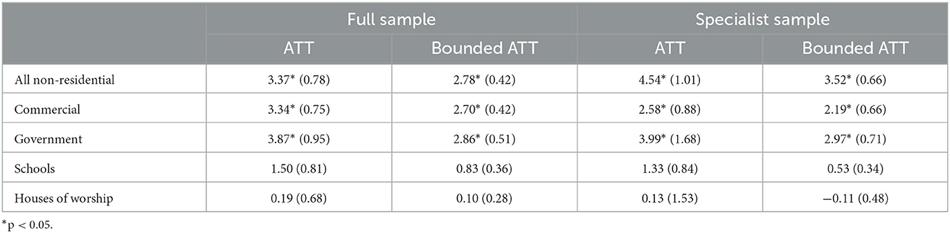
Table 3. Average treatment effects from staggered difference-in-differences (group-time standard errors in parentheses).
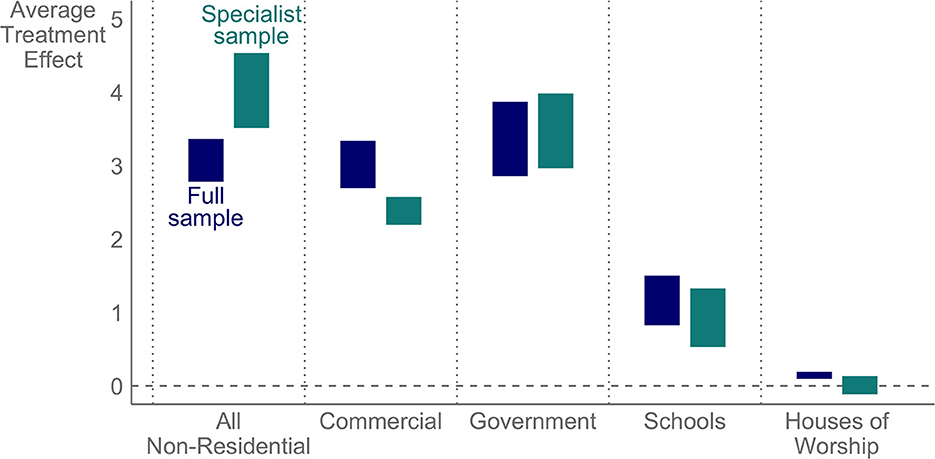
Figure 2. Average treatment effects (ATT) across model specifications and data samples. Boxes are based on the range between the ATT and the bounded ATT described in Equation 2.
As already noted, the results are not perfectly comparable across the four building types. One issue is the substantial differences in sample sizes, and in particular the smaller sample associated with the school and houses of worship samples. Further, the “treatment” can entail different numbers of installations across the building types. In the treated groups there is an average of 11.8 commercial installs per zip code, compared to 1.6 house-of-worship installs, for instance. One way to level the results across the types is to estimate the total number of influenced residential adoptions per non-residential installation in each group. That is, we divide the group-level treatment effects by the number of non-residential installations in each group and take the average for all positive treatment effects. Based on the specialist sample, we estimate that each commercial install influences around 0.06 installs per quarter, each government and school install influences around 0.3 installs per quarter, and each house-of-worship install influences around 1.2 installs per quarter. This comparison is still imperfect, since the smaller numbers of school and house-of-worship installs inflate the per-install estimates even if the overall treatment effect is the same. Still, this analysis suggests that the school and house-of-worship influence per install is more comparable to the other types than the aggregate results in Table 3 would suggest.
The individual group-time effects are also of interest to show how influence effects may vary over time. To visualize these results, we calculated average group-time effects based on the elapsed number of quarters from treatment. For instance, for the group of zip codes where a non-residential system was first installed in quarter 5, the elapsed quarters in quarter 5 is 0, the elapsed quarters in quarter 6 is 1, the elapsed quarters in quarter 10 is 5, and so on. Conversely, elapsed quarters are negative in quarters preceding the first non-residential installation.
Figure 3 depicts the average group-time effects by elapsed quarters for 5 years before and after non-residential system installations (20 elapsed quarters). The group-time effects mostly vary around zero prior to the non-residential installations (negative elapsed quarters). The consistently positive group-time effects after the zero mark provide a visual depiction of the influence effects. The average treatment effects are effectively aggregate values of the points to the right of zero depicted in Figure 3.
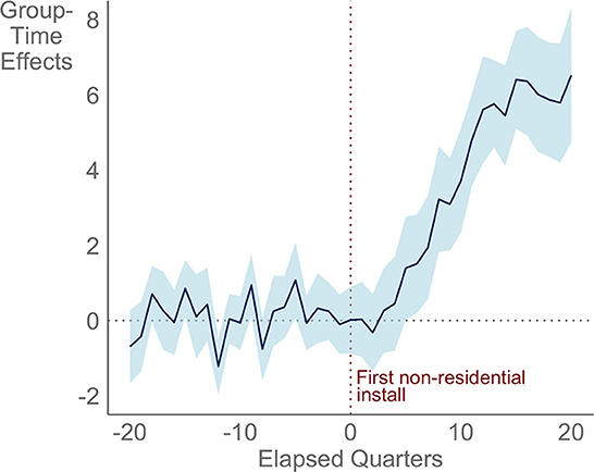
Figure 3. Group-time effects by number of quarters elapsed from non-residential installation. Based on specialist installer data samples.
The fact that the group-time effects are consistently positive after non-residential installs supports the premise that PV influence is a continuous, long-term process. All three of the non-residential types exhibit similar temporal trends as the full non-residential sample, with group-time effects gradually increasing over time. We posit several explanations for why the group-time effects tend to grow over time. First, influence effects likely correlate with underlying propensities to adopt. For instance, a household with a low preexisting adoption propensity is less likely to be influenced to adopt by seeing an installed system than a household that was already considering adoption, all else equal. Aggregate propensities to adopt have likely increased over time as PV prices declined and households became more aware of rooftop PV. These increasing propensities to adopt could mean growing impacts from PV influence. Households may therefore become more likely to adopt in response to an external influence. Second, when a non-residential install influences a household to adopt, that household's installed system becomes another source of influence. As a result, increasing group-time effects could reflect the accumulating influence effects of previously influenced adoptions. Third, growing influence over time may reflect the accumulating effects of multiple non-residential systems in the same zip code.
The fact that group-time effects increase over time means that the average treatment effects are potentially sensitive to spurious long-term trends in adoption. To test the dependence of the results on potentially spurious long-term trends, we use a decay rate to weight the group-time effects by time. The decay rate effectively measures the rate at which we assume true influence wanes over time. The results for all non-residential systems in the model are statistically significant up to a decay rate of 68%, suggesting that the results are robust assuming that true influence wanes by <68% per quarter.
Table 4 presents the results of several alternative models as robustness checks to our preferred results in Table 3. All the robustness checks follow the same structure described in Section 3 and are based on the non-residential specialist installer subsample. We implement the following robustness checks:
a) This model uses TTS rather than BuildZoom data for residential adoptions (N = 6,313 non-residential installations, 1,241,160 residential adoptions). As discussed in Section 3.1, we prefer the BuildZoom data since those data include better proxies for adoption dates. However, we can increase the residential adopter sample by about 20% by using the interconnection dates in the TTS data. To bring those dates closer to adoption dates, we adjust each interconnection date 68 days backwards, the median duration between contract signature and interconnection as estimated by NREL (2023).
b) This model restricts the geographic sample to zip codes with at least 100 non-residential establishments (N = 4,799 non-residential installations, 953,220 residential adoptions). The rationale is that zip codes with few non-residential establishments are more likely to be allocated to the control group and could vary in confounding ways from other zip codes. Restricting the sample to zip codes with at least 100 non-residential establishments should mitigate that confounding variation. We identify the subsample using U.S. Census zip code business pattern data.
c) This model converts the dependent variable to a residential adoption rate (number of adoptions per 1,000 households) rather than the adoption level (number of adoptions). We exclude the number of households from the control group in these models.
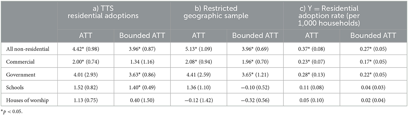
Table 4. Average treatment effect robustness checks (group-time standard errors in parentheses).
The results are largely robust across the alternative models. Consistent with our preferred results in Table 3, the results are consistently positive and statistically significant in the larger samples (all non-residential, commercial, government). Results are either weakly significant or insignificant for the smaller samples (schools, houses of worship).
Our second research question is whether non-residential influence effects vary substantially from residential influence. The literature does not provide strong a priori theories about such deviations. On the one hand, non-residential influence effects may be stronger than residential influence if factors such as visibility, installed capacity, and community leadership are central mechanisms in influenced adoption. On the other hand, non-residential influence may be relatively weaker if peer influence is the key mechanism, i.e., if households respond more strongly to the behavior of other households rather than non-residential actors.
We explored the possibility of comparing residential and non-residential influence effects using established methods for PV peer effects estimation, to directly compare our results with previous peer effect estimates. We encountered two challenges. First, the non-residential market is about an order of magnitude smaller than the residential market. As a result, differences in estimated effects could be affected by differences in the consistency of the estimates. Coefficient consistency is further reduced by fixed effects, a critical component in residential peer effect models (Bollinger and Gillingham, 2012). Second, non-residential installation variables are highly collinear with the residential installation variables. Severe multicollinearity inflates the variance of non-residential coefficients in models that include residential installations. For both reasons, typical PV peer effect models yield highly inconsistent estimates for non-residential influence effects.
Instead, we use the same DiD approach described in Section 3.2 to compare the magnitudes of residential and non-residential influence effects. We lack clear market discontinuities in the residential context like those we used in the non-residential context. Still, residential influence effects could be estimated from exogenous shocks to residential deployment rates. To establish some intuition behind this approach, suppose a researcher persuaded a set of random households in different zip codes to install rooftop PV. The researcher could then explore changes in residential adoption trends in this hypothetical treatment group. We use the marketing activities of large, national-scale installers to replicate this hypothetical experiment. Specifically, we use installations by the two largest residential PV installers, Sunrun and Tesla. When these installers “enter” a zip code they compete with established local installers. Available evidence suggests that market entry is not zero sum, such that market entry increases local adoption rates (O'Shaughnessy et al., 2023). As a result, the market entrance of a national-scale installer represents a shock to the local market. We use these shocks to estimate residential influence effects. Building on the approach described in Section 3.2, we restrict our data sample to zip codes where Sunrun/Tesla had installed no systems prior to 2010. We then identified a treatment group comprising zip codes where Sunrun or Tesla entered at some point during the study period (N = 1,498 zip codes). We built control groups using the same propensity score matching process already discussed. Again, we use staggered DiD to measure differences in adoption rates after Sunrun/Tesla had entered local markets.
The estimated average treatment effect for the residential model is 6.3 (SE = 1.2). That estimate includes adoptions for systems installed by Sunrun/Tesla, some of which may reflect influence while others may reflect exogenous market decisions. To estimate a lower-bound on residential influence, we removed adoptions associated with Sunrun/Tesla to prevent conflating trends in installer marketing patterns with influence. That is, we effectively measure the impacts of Sunrun/Tesla installations on adoption rates associated with other installers. The estimated influence effect in the restricted model is 2.9 (SE = 0.3) (Figure 4), with evidence of a weak pre-trend (0.06). The result is similar in magnitude to the non-residential effects in Table 3, though the effects are not perfectly comparable. The Sunrun/Tesla systems tend to be installed in much larger clusters than the non-residential installs. One way to yield a better comparison is to restrict the Sunrun/Tesla samples such that the number of installs per treated zip code is closer to the same metric in the non-residential samples. Restricting the residential sample such that the number of Sunrun/Tesla installs per zip code is slightly less than the number of non-residential installs per zip code in the specialist sample, the estimated residential influence effect falls just slightly to 2.1 (SE = 0.4). The residential influence effects similarly increase over time, consistent with the trends depicted in Figure 3. Hence, the analysis suggests that non-residential influence effects are of the same order of magnitude as residential influence. These results accord with Baranzini et al. (2017), who similarly find that residential and non-residential installs are associated with comparable increases in residential adoption rates.
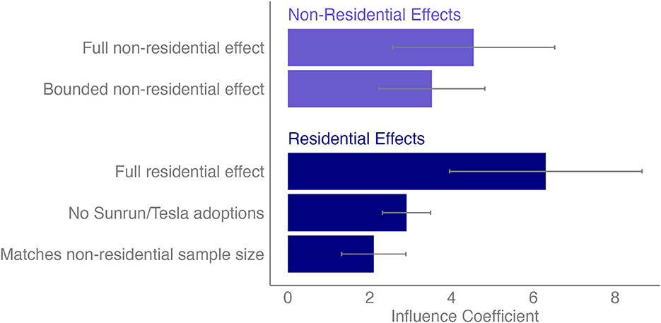
Figure 4. Comparison of estimated non-residential and residential influence coefficients. Non-residential estimates based on specialist sample.
Our results suggest that non-residential PV installations are associated with local increases in residential adoption rates. Our results broadly support two conclusions: (1) that non-residential installations accelerate residential adoption; (2) that the magnitude of influence from non-residential PV installs is roughly comparable to effects from residential installs. We discuss and explore the implications of each of these conclusions in turn.
First, our results suggest that non-residential installations influence residential PV adoption decisions. From a policy perspective, the results suggest that policy-enabled non-residential installations could “seed” rooftop PV adoptions. This concept has been proposed as an approach for accelerating low-income PV adoption. The idea is that low-income neighborhoods with limited or no PV installations also have limited or no sources of PV influence, serving as an additional barrier to low-income adoption. Policymakers interested in driving low-income rooftop PV adoption, for example, could potentially facilitate low-income adoption by enabling non-residential installations in low-income neighborhoods. Houses of worship may be a particularly effective non-residential building type to influence low-income adoption given evidence on house-of-worship influence in low-income communities (Joshi et al., 2009) and the role of houses of worship in the implementation of public programs (Evans and Hudson, 2014; Flórez et al., 2017). However, it is unclear how effective such interventions would be without directly addressing low-income barriers to solar adoption (e.g., budget constraints, lower home ownership rates). Further, the results suggest that governments could lead by doing: the government influence effect estimates suggest that rooftop PV installed on government buildings drives residential PV adoption. The efficacy of seeding policies could be increased with more precise knowledge of the mechanisms of non-residential PV influence. For instance, if active influence is more important, policymakers could collaborate with institutions that can maximize active influence in the community, such as houses of worship. Alternatively, if passive influence mechanisms such as visibility are more important, policymakers could seed rooftop PV adoption by subsidizing non-residential PV on visibly prominent rooftops or in city centers. Policymakers could potentially foment passive influence through other measures to enhance visibility, such as public certifications like plaques for building LEED certification. Understanding the precise mechanisms of PV influence is a proposed area for further research.
Second, we find that non-residential influence effects are comparable to residential influence effects. This conclusion is based on an imperfect comparison, given that we cannot isolate the impacts of individual residential systems as effectively as for non-residential systems. Still, broadly speaking, our results indicate that residential and non-residential influence effects are on the same order of magnitude, the same conclusion reached by Baranzini et al. (2017). The comparability of the results suggests shared mechanisms of PV influence. The most straightforward shared mechanism is visibility. Previous work shows that visibility plays a key role in PV influence (Bollinger et al., 2022), and could likewise drive non-residential influence effects given the relatively large sizes and prominent locations of non-residential PV systems.
Our results also suggest that non-residential influence effects may vary across non-residential building types, though further research is required. Specifically, the estimated influence effects of government systems are generally larger than those of commercial systems. These differences suggest that building type or use may mediate the extent of influence. For instance, it is possible that buildings that provide spaces of public interaction—including many government buildings and houses of worship—generate more influence than other spaces. Stronger influence from government buildings would be consistent with previous work showing that local governmental decisions influence private action, such as how government investments in green buildings can drive similar investments in the private sector (Koski and Lee, 2014). Further, there are theoretical reasons to expect stronger influence from certain institutions, especially schools and houses of worship. Schools often have direct interactions with communities in ways that could enhance influence (Keyes and Soleil, 2001). Houses of worship are community institutions that directly interact with their congregations, establish social cohesion, and can influence behavior. Houses of worship have been shown to actively influence their congregations, such as by driving pro-animal welfare behavior (Brown, 2019), healthy lifestyles (Krause et al., 2010), and prosocial behavior (Van Cappellen et al., 2016). Houses of worship that adopt PV could similarly actively influence PV adoption in their congregations, especially among houses of worship that profess environmental and sustainability values (Yale, 2022). This hypothesis is borne out in groups such as Green the Church and Interfaith Power and Light who promote rooftop PV adoption among houses of worship and environmental education for congregations. Whether certain institutions achieve greater influence through existing social linkages is another proposed area for future research. Differences across building types may also reflect architectural differences. For instance, installations on shorter non-residential buildings with street-facing roofs may be more influential than installations on taller buildings or on buildings with architectural features that block panels. The effects of architecture on solar influence are an area for further research.
Finally, our results suggest a broader understanding of PV influence than has generally been considered in the literature to date. We find clear evidence of associations between adoptions across customer types, suggesting that influence need not have a peer-to-peer basis as typically assumed in discussion of residential peer effects models. Further, we model influence as a continuous, long-term process. We find evidence that influence effects increase over time. We posit that increasing influence could reflect temporal trends in propensities to adopt. We also posit that influence can accumulate over time, partly because an influenced adoption in one time period is a source of potential influence in subsequent time periods. Future research could decompose the component parts of influence effects to better understand the long-term role of influence on PV adoption.
The original contributions presented in the study are included in the article/supplementary material, further inquiries can be directed to the corresponding author.
EO'S, GB, and AG contributed to conception and design of the study. EO'S and AG collected and organized the data. EO'S performed the statistical analysis and wrote the first draft of the manuscript. All authors contributed to manuscript revision, read, and approved the submitted version.
This material is based upon work supported by the U.S. Department of Energy's Office of Energy Efficiency and Renewable Energy (EERE) under the Solar Energy Technologies Office Award Number 38444 and Contract No. DE-AC02-05CH11231.
The authors would like to thank Interfaith Power and Light for providing data to support this study. The authors would also like to thank Sydney Forrester and Joyce McLaren for inputs to this study.
The authors declare that the research was conducted in the absence of any commercial or financial relationships that could be construed as a potential conflict of interest.
The authors IF-W and EO'S declared that they were an editorial board member of Frontiers, at the time of submission. This had no impact on the peer review process and the final decision.
All claims expressed in this article are solely those of the authors and do not necessarily represent those of their affiliated organizations, or those of the publisher, the editors and the reviewers. Any product that may be evaluated in this article, or claim that may be made by its manufacturer, is not guaranteed or endorsed by the publisher.
The views expressed in the article do not necessarily represent the views of the DOE or the U.S. Government. The U.S. Government retains and the publisher, by accepting the article for publication, acknowledges that the U.S. Government retains a non-exclusive, paid-up, irrevocable, worldwide license to publish or reproduce the published form of this work, or allow others to do so, for U.S. Government purposes.
1. ^Throughout this paper, the term “non-residential” refers exclusively to PV adopted by a single non-residential electricity customer, as distinguished from utility-scale PV which is operated by electric utilities to serve ratepayers, or community PV which serves multiple customers.
2. ^See https://www.interfaithpowerandlight.org/congregational-solar/.
3. ^See melissa.com for more information on the address verification service. Note that a similar confirmation was not required for the other non-residential systems which are confirmed as non-residential during the data collection process.
4. ^Peer effect models are commonly specified using adoption rates (number of adoptions per household). We chose to implement the models in terms of adoption levels to simplify the interpretation of the results. We present results for models in terms of adoption rates as a robustness check in Section 4.2.
5. ^We exclude this value from the propensity score matching because the value and type of incentives are not comparable across states. For instance, the value of an up-front rebate in one state is not directly comparable to the long-term value of a production-based incentive ($/kWh of output) in another state.
6. ^This adjustment yields more conservative results. Unlike the other cases, where the specialist sample generates smaller coefficients, the house-of-worship specialist sample (N = 70) yielded influence effect coefficients that were larger than other results presented in Table 3. While it is possible that these larger results reflect substantial influence in that subsample, the larger effects do not hold across the larger sample of houses of worship.
Alipour, M., Salim, H., Steward, R. A., and Sahin, O. (2020). Predictors, taxonomy of predictors, and correlations of predictors with the decision behaviour of residential solar photovoltaics adoption: a review. Renew. Sust. Energ. Rev. 123, 109749. doi: 10.1016/j.rser.2020.109749
Axsen, J., and Kurani, K. S. (2012). Social influence, consumer behavior and low-carbon energy transitions. Ann. Rev. Environ. Res. 37, 311–340. doi: 10.1146/annurev-environ-062111-145049
Balta-Ozkan, N., Yildirim, J., Connor, P. M., Truckell, I., and Hart, P. (2021). Energy transition at local level: analyzing the role of peer effects and socio-economic factors on UK solar photovoltaic deployment. Energy Policy 148, 112004. doi: 10.1016/j.enpol.2020.112004
Baranzini, A., Carattini, S., and Péclat, M. (2017). What Drives Social Contagion in the Adoption of Solar Photovoltaic Technology? London: Grantham Research Institute on Climate Change and the Environment.
Barbose, G., Darghouth, N., O'Shaughnessy, E., and Forrester, S. (2021). Tracking the Sun: Pricing and Design Trends for Distributed Photovoltaic Systems in the United States. Berkeley, CA: Lawrence Berkeley National Laboratory.
Bollinger, B., and Gillingham, K. (2012). Peer effects in the diffusion of solar photovoltaic panels. Marketing Sci. 31, 900–912. doi: 10.1287/mksc.1120.0727
Bollinger, B., Gillingham, K., Kirkpatrick, A. J., and Sexton, S. (2022). Visibility and peer influence in durable good adoption. Market. Sci. 4, 453–476. doi: 10.1287/mksc.2021.1306
Brown, J. E. (2019). Can christian worship influence attitudes and behavior toward animals. J. Anim. Ethics 9, 47–65. doi: 10.5406/janimalethics.9.1.0047
Callaway, B., and Sant'Anna, P. H. C. (2021). Difference-in-differences with multiple time periods. J. Econ. 225, 2. doi: 10.1016/j.jeconom.2020.12.001
Carley, S., Engle, C., and Konisky, D. M. (2021). An analysis of energy justice programs across the United States. Energy Policy 152, 112219. doi: 10.1016/j.enpol.2021.112219
Carlisle, J. E., Solan, D., Kane, S. L., and Joe, J. (2016). Utility-scale solar and public attitudes toward siting: a critical examination of proximity. Land Use Policy 58, 491–501. doi: 10.1016/j.landusepol.2016.08.006
Davis, M., White, B., Goldstein, R., Leyva Martinez, S., Chopra, S., Goss, K., et al. (2022). US Solar Market Insight: 2021 Year in Review. New York, NY: Wood Mackenzie.
Evans, K. R., and Hudson, S. V. (2014). Engaging the community to improve nutrition and physical activity among houses of worship. Prev. Chronic Dis. 11, 130270. doi: 10.5888/pcd11.130270
Flórez, K. R., Payán, D. D., Derose, K. P., Aunon, F. M., and Bogart, L. M. (2017). Process Evaluation of a peer-driven, HIV stigma reduction and HIV testing intervention in latino and African American churches. Health Equity 1, 109–117. doi: 10.1089/heq.2017.0009
Graziano, M., and Gillingham, K. (2015). Spatial patterns of solar photovoltaic system adoption: the influence of neighbors and the built environment. J. Econ. Geograph. 15, 815–839. doi: 10.1093/jeg/lbu036
Ho, D., Imai, K., King, G., and Stuart, E. (2011). MatchIt: nonparametric preprocessing for parametric causal inference. J. Stat. Software 42, 1–28. doi: 10.18637/jss.v042.i08
Huggins, J. (2022). U.S. Electric Utility Companies and Rates: Look-up by Zipcode. Golden, CO: N. R. E. Laboratory.
Joshi, P., Hardy, E., and Hawkins, S. (2009). Role of Religiosity in the Lives of the Low-Income Population: A Comprehensive Review of the Evidence. Washington, DC: Department of Health & Human Services.
Keyes, M. C., and Soleil, G. (2001). School-Community Connections: A Literature Review. Institute of Education Sciences: Washington, DC.
Koski, C., and Lee, T. (2014). Policy by doing: formulation and adoption of policy through government leadership. Policy Stu. J. 42, 30–54. doi: 10.1111/psj.12041
Krause, N., Shaw, B., and Liang, J. (2010). Social relationships in religious institutions and healthy lifestyles. Health Educ. Behav. 38, 25–38. doi: 10.1177/1090198110370281
Manski, C. F., and Pepper, J. V. (2018). How do right-to-carry laws affect crime rates? Coping with ambiguity using bounded-variation assumptions. The Rev. Econ. Stat. 100, 232–244. doi: 10.1162/REST_a_00689
Moezzi, M., Ingle, A., Lutzenhiser, L., and Sigrin, B. (2017). A Non-Modeling Exploration of Residential Solar Photovoltaic Adoption and Non-Adoption. Golden, CO: National Renewable Energy Laboratory.
Mundaca, L., and Samahita, M. (2020). What drives home solar PV uptake? Subsidies, peer effects and visibility in Sweden. Energ. Res. Soc. Sci. 60, 101319. doi: 10.1016/j.erss.2019.101319
O'Shaughnessy, E., Forrester, S., and Barbose, G. (2023). Supply sunspots and shadows: business siting patterns and inequitable rooftop solar adoption in the United States. Energ. Res. Soc. Sci. 96, 102920. doi: 10.1016/j.erss.2022.102920
Palm, A. (2017). Peer effects in residential solar photovoltaics adoption - A mixed methods study of Swedish users. Energ. Res. Soc. Sci. 26, 1–10. doi: 10.1016/j.erss.2017.01.008
Rambachan, A., and Roth, J. (2022). An Honest Approach to Parallel Trends. Advances in Differences-in-Differences. New York, NY: American Economic Assocation.
Richter, L. L. (2013). Social Effects in the Diffusion of Solar Photovoltaic Technology in the UK. Cambridge, MA: Energy Policy Research Group Working Paper, University of Cambridge.
Schulte, E., Scheller, F., Sloot, D., and Bruckner, T. (2022). A meta-analysis of residential PV adoption: the important role of perceived benefits, intentions and antecedents in solar energy acceptance. Energ. Res. Soc. Sci. 84, 102339. doi: 10.1016/j.erss.2021.102339
Sigrin, B., Dietz, T., Henry, A., Ingle, A., Lutzenhiser, L., Moezzi, M., et al. (2017). Understanding the Evolution of Customer Motivations and Adoption Barriers in Residential Solar Markets: Survey Data. Golden, CO: N. R. E. Laboratory.
Sigrin, B., Sekar, A., and Tome, E. (2022). The solar influencer next door: predicting low income solar referrals and leads. Energ. Res. Soc. Sci. 86, 102417. doi: 10.1016/j.erss.2021.102417
Sintov, N. D., and Schultz, P. W. (2015). Unlocking the potential of smart grid technologies with behavioral science. Front. Psychol. 6, 410. doi: 10.3389/fpsyg.2015.00410
Tamer, E. (2010). Partial identification in econometrics. Ann. Rev. Econ. 2, 167–195. doi: 10.1146/annurev.economics.050708.143401
Van Cappellen, P., Saroglou, V., and Toth-Gauthier, M. (2016). Religiosity and prosocial behavior among churchgoers: exploring underlying mechanisms. The Int. J. Psychol. Relig. 26, 19–30. doi: 10.1080/10508619.2014.958004
Wolske, K., Gillingham, K., and Schultz, W. (2020). Peer influence on household energy behaviours. Nat. Energ. 5, 202–212. doi: 10.1038/s41560-019-0541-9
Xiong, H., Payne, D., and Kinsella, S. (2016). Peer effects in the diffusion of innovations: theory and simulation. J. Behav. Exp. Econ. 63, 1–13. doi: 10.1016/j.socec.2016.04.017
Yale (2022). Religious Ecojustice Bibliography. Yale Forum on Religion and Ecology. Available online at: https://fore.yale.edu/sites/default/files/files/Religious%20Ecojustice%20Bibliography(2).pdf
Keywords: solar, adoption, influence, behavior, peer effects
Citation: O'Shaughnessy E, Barbose G, Grayson A, Ferrall-Wolf I and Sunter D (2023) Impacts of non-residential solar on residential adoption decisions. Front. Sustain. Energy Policy 2:1203517. doi: 10.3389/fsuep.2023.1203517
Received: 10 April 2023; Accepted: 23 October 2023;
Published: 16 November 2023.
Edited by:
Anna Ebers Broughel, Johns Hopkins University, United StatesReviewed by:
Parth Vaishnav, University of Michigan, United StatesCopyright © 2023 O'Shaughnessy, Barbose, Grayson, Ferrall-Wolf and Sunter. This is an open-access article distributed under the terms of the Creative Commons Attribution License (CC BY). The use, distribution or reproduction in other forums is permitted, provided the original author(s) and the copyright owner(s) are credited and that the original publication in this journal is cited, in accordance with accepted academic practice. No use, distribution or reproduction is permitted which does not comply with these terms.
*Correspondence: Eric O'Shaughnessy, ZW9zaGF1Z2huZXNzeUBsYmwuZ292
Disclaimer: All claims expressed in this article are solely those of the authors and do not necessarily represent those of their affiliated organizations, or those of the publisher, the editors and the reviewers. Any product that may be evaluated in this article or claim that may be made by its manufacturer is not guaranteed or endorsed by the publisher.
Research integrity at Frontiers
Learn more about the work of our research integrity team to safeguard the quality of each article we publish.