Water quality mitigation strategy analysis of the Salton Sea, California, using the Delft-3D modeling suite

The Salton Sea is the largest lake in California and is a shallow, hypersaline lake. The endorheic lake has been significantly maintained by agricultural return flows from Imperial Valley farming and two rivers- the New River and Alamo River- which originate in Mexicali, Mexico. The current salinity is at 74 ppt and is expected to increase due to the Quantification Settlement Agreement signed in 2003, stipulating the transfer of nearly 0.616 km³ per year of Colorado River water to urban areas for up to 75 years. This has resulted in inflows reduction, and the dust storms created by the dried-up playa have become a prominent risk to public health in the region. Massive fish and bird kills began in the 1980s and continued to occur periodically. In this study, the Delft3D numerical modeling suite- FLOW, WAVE, and WAQ- was utilized to investigate the transport and cycling of nutrients under the influence of wind-induced sediment resuspension activity. The three-dimensional hydrodynamic and water quality combined model was applied to simulate mitigation scenarios to assess long-term effects on salinity and water quality of (1) emerged islands as a nature-based solution, (2) seawater import/export, and (3) seawater import/export in addition to treating tributary rivers to remove nutrients. Overall, this study supported the findings from previous studies and showed that sediment resuspension is the driving force for nutrients cycling in the water column and that emerged islands have long-term potential to enhance burial activity for pollutants removal in the Salton Sea. Furthermore, the seawater import/export scenario showed promising results of reducing salinity level from 46 ppt to 38–39 ppt in 2 years. The 3D numerical hydrodynamic/water quality model developed in this work is the first and latest integrated modeling approach tailored to the Salton Sea's system and has the capacity to improve understanding of the complicated water quality dynamics changes in various restoration concepts. This study demonstrated that being able to explore the full potentials of restoration designs using a comprehensive 3D water quality modeling framework is critical in achieving wholesome planning that will create environmental, social, and economic benefits in the long term for the Salton Sea.

1. Introduction

The Salton Sea is a terminal hypersaline lake located in the southeast of the famous desert resort city of Palm Springs. It is 56 km north of the U.S.-Mexico border in southern California, USA (Figure 1). The terminal lake's succession has been determined by the change of course of the Colorado River over the past several thousand years. However, in 1905, an irrigation canal failure in the Imperial Valley caused the river to overflow the Salon Sink for 2 years intermittently, thus creating the waterbody of the modern Salton Sea (Setmire et al., 1990; Cohen et al., 1999).

FIGURE 1

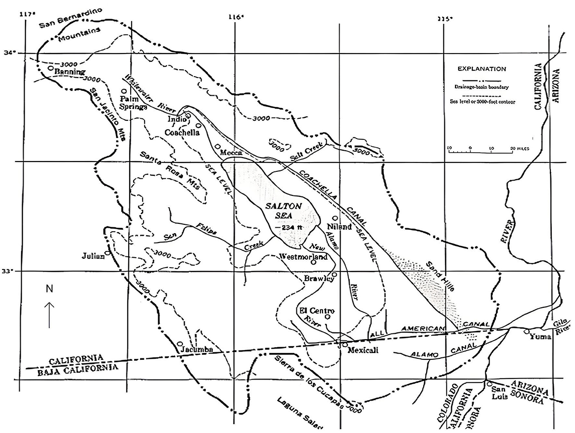
Figure 1. The Salton Sea transboundary watershed and the tributary rivers. Figures obtained from Hely et al. (1966).

Massive fish and bird kills began in the 80s due to toxic algae contamination and low dissolved oxygen. Moreover, the ecological crisis has been exacerbated since the Quantification Settlement Agreement (QSA) was signed in October 2003. The Imperial Irrigation District, the agency that controls the bulk of the agricultural allocation within the Lower Colorado River Basin's annual water allocation, agreed to transfer 0.246 km³a⁻¹ of water to San Diego County Water Authority by 2021 until at least 2077, 0.0616 and 0.123 km³a⁻¹ to Coachella Valley Water District and Metropolitan Water District by 2018, respectively, until at least 2077 (Hughes, 2020). As of 2018, roughly 38.4% annual reduction of inflow water has led to the rapid decline of the Salton Sea's water level, exposing land previously underwater. This dried-up playa has created airborne dust storms and becomes a public health hazard that affects the population around the Sea (Farzan et al., 2019).

As of the current time (August 2023), the water level has decreased approximately 3.5 meters (−73.3 m) since the execution of the QSA in 2003 (−69.7 m) and 1.38 meters since the end of the mitigation flows in 2018 (−71.9 m), exposing 127 km² of the lakebed. The Sea started as the largest freshwater lake in California, then from the 1940s, the salinity level reached the same as the Pacific Ocean (35 ppt) and exceeded it from the 1960s (Barnum et al., 2017). Today, the salinity has increased from approximately 46 ppt in 2005 to approximately 74 ppt in early 2020 and is expected to continue to rise. The increase in salinity has nearly eliminated the Tilapia and its two prey species-Pupfish and Sailfin Mollies- the primary food source for most of the birds that visit the Sea. Based on the study done by the Little Hoover Commission, it was projected that by 2023, the elevation would drop to approximately −73.7 meters below sea level, the salinity would reach 70 ppt, and Tilapia and its two prey species would die out. The observed changes in the current Salton Sea approximately match the projections as of early 2023 (Little Hoover Commission, 2015).

The Salton Sea has previously functioned as a significant stopover for migratory birds on the Pacific Flyway for more than 400 species and was designated an Audubon Important Bird Area of global significance (Barnum et al., 2017). After numerous severe fish and bird die-offs since the 80s, the Sea is now named “IBA in Danger” (Important Bird & Biodiversity Area) by BirdLife International. Additionally, it is believed that the dust periodically transported off the exposed Salton Sea lakebed is the main reason for Coachella and Imperial County's high asthma and cardiovascular disease rate. The visit record of the asthma emergency department in 2014 showed that the visiting rate of children in Imperial County was among the highest in California and about 1.8 times the state average (Farzan et al., 2019; California Department of Public Health, n.d.).

The Salton Sea is a wind-driven system; the frequency, strength, duration, the timing of wind events, along with its unique bathymetry, play significant roles in determining the biogeochemical cycles in the waterbody. Previous studies have suggested that the eutrophication occurring in the Salton Sea is heavily influenced by the diffusive fluxes of nutrients from sediments (internal loading) within the water column, and sediment resuspension caused by wind-induced wave activity is the dominant mechanism for the Salton Sea's nutrient cycling (Chung et al., 2008, 2009a). In addition, Marti-Cardona et al. (2008) showed that wind-driven upwellings of hypolimnetic water in the Salton Sea during thermal stratification were directly linked to fish kills.

To demonstrate the effects of formerly proposed restoration configurations that aim to tackle the rising salinity concern of the Salton Sea, previous research groups had conducted hydrodynamic simulations of the Salton Sea in the early 2000s to simulate its circulation/thermal conditions, including RMA10 (Cook et al., 2002), Dynamic lake model-water quality, DLM-WQ (Chung et al., 2008, 2009a) and a three-dimensional numerical model (Si3D) (Rueda et al., 2009). Among these, Chung et al. (2009a) made the first attempt combining sediment resuspension models with a process-based, Lagrangian layer schemed, one-dimensional hydrodynamic/water quality model (DLM-WQ) to investigate the effect of sediment resuspension on nutrient cycling in the Salton Sea. The water quality simulation results showed that nutrient concentration would increase due to higher sediment resuspension events, and the Sea would have stronger stratification for longer periods in reduced sizes. All previous Salton Sea models were developed and calibrated based on 1 year of complete temperature and water quality data collected in 1997. The water quality simulation was based on a one-dimensional assumption that was not built to simulate salinity higher than 44 ppt (Chung et al., 2008).

In recent decades, the government has shifted focus and proposed to implement a sequence of dust suppression and habitat restoration projects around the perimeter of the Salton Sea to address air quality and ecological threats due to the projected decline of the Sea. However, previous evaluation has suggested that the Salton Sea would shrink and become more saline, and the current problematic nutrients loading schemes will remain the same regardless of whether the perimeter habitats are implemented or not (Reclamation, 2007). As a result, the objective of this study is to propose water quality mitigation strategies for the Salton Sea based on the principle that its nutrient cycle is primarily driven by wind-driven sediment resuspension events.

In this study, the Delft3D (Deltares, Delft, The Netherlands) modeling suite was chosen as the numerical model to conduct hydrodynamic and water quality/sediment resuspension simulations in the Salton Sea. The three models most relevant to our study within the Delta Shell framework include Delft3D-FlOW, Delft3D-Waves, and Delft3D-WAQ. Each module has its conceptual design and numerical implementations; Delta Shell is a mutual interface where multiple modules can be integrated and carry out 3D simulations for non-steady flow and transport phenomena/water quality processes resulting from meteorological forcing.

This study is the first attempt to utilize a three-dimensional, numerical hydrodynamics/water quality model to characterize the Salton Sea's hydrodynamics and nutrient cycling in the water column and sediment-water interaction. In addition, the model was calibrated and validated using the datasets measured from August 8 to September 17, 2005, by Chung et al. (2009b). The validation period of 9/1/2005 to 8/8/2007 is the longest simulation on the hydrodynamics and water quality of the Salton Sea performed so far. The validated models were used to simulate three water quality mitigation scenarios, including building emerged islands, seawater import/export canal implementation, and seawater canal construction in addition to treated tributary rivers (90% nutrient reduction).

This study confirmed that sediment resuspension is the main factor influencing orthophosphate concentration in the water column. Based on this principle, emerged islands that serve to reduce wind-induced bottom shear stress, thereby reducing sediment resuspension effects, were designed as a nature-based solution. The simulation indicated that the area covered by the emerged islands shields the bottom from shear stress exceeding the critical level, which could enhance burial effects that lead to significant orthophosphate removal in the water column. In the long term, the built environment provides low-impact resilience to wind-driven bottom shear stress that can improve water quality without having the potentially detrimental consequences from disturbed natural lake stratification. Furthermore, the seawater import/export mitigation scenario showed promising results of lowering contaminants such as unionized ammonia and chlorophyll a and reducing salinity levels from 46 ppt to 38–39 ppt in 2 years. Overall, this work demonstrated the capacity of a comprehensive, three-dimensional water quality/hydrodynamic model in simulating water quality dynamics of the Salton Sea in various configurations/management actions and advocated the vital role of a high-level water quality model in future planning for the restoration of the Salton Sea.

2. Materials and methods

2.1. Study area

The Salton Sea is the largest lake in California, located in the US-Mexico transboundary region, with a surface area of approximately 823 km² (as of early 2023). It is a shallow lake with a mean depth of 8 m and a maximum depth of 15 m (Watts et al., 2001; Holdren and Montaño, 2002). Situated below sea level in the valley, the arid climate and unique geographical conditions have shaped the used-to-be freshwater lake into an endorheic and hypersaline lake. The Salton Sea belongs to the Colorado River Basin-Region 7 as the Colorado River flows across the border through Mexicali for 25 km, then the two tributary rivers- the New and Alamo rivers- flow northward into the basin through the vest Farming region before draining into the terminal in the Imperial County (Figure 1) (Hely et al., 1966; U.S. EPA, 2005).

The Salton Sea was designated as an agricultural wastewater sump since the mid-1920s. Before the QSA took official effect in 2018, the Sea's water level had been maintained by the inflows of the New and Alamo rivers from Imperial County/Mexicali and the Whitewater River from Riverside County. Among these, the two rivers discharging into the south end of the Sea have been identified as impaired waters under section 303 (d) of the Federal Clean Water Act and contributed about 75% of the inflow to the Sea. The Whitewater River's contribution (~4% of total inflows) was relatively insignificant. The New River contains industrial/agricultural runoff (51.2% on the Mexico side, 18.4% on the U.S. side) and sewage discharge from Mexicali (29%) with a flow rate of approximately 16 to 20 m³s⁻¹. On the other hand, the Alamo River is dominated by agricultural return flows from the Imperial Valley, with a higher flow rate of 19 to 26 m³s⁻¹ (RWQCB, 1998).

2.2. Salton Sea's physical and chemical characteristics

The Salton Sea region has significant seasonal air temperature, solar radiation, and wind speed differences. From 2018 to 2022, the minimum mean air temperature recorded at the southwestern end of the Sea was 4°C in January, and the maximum mean was 40°C during the summer months (June–August). The wind speeds recorded off the coast in the southwestern corner of the Salton Sea showed that the predominant and strongest winds were from the west (240°-280°) and reached 15–20 m/s on average from 2015 to 2019, while the weakest wind was recorded in the land-based station located at the north end of the Sea with the 5-year average wind speed below five m/s from the south (~180°). The spring season (March–May) consistently had the highest mean wind speeds above 15 m/s, and the winter season (October–January) experienced strong winds occasionally based on the records from 2015 to 2019 (Lee, 2021).

The Sea is a wind-driven system; wind events' frequency, strength, duration, and timing cause significant variations in lake dynamics in different years. Wind-generated turbulence can diminish heat loss via back radiation and increase heat gain via conduction. In the spring season, strong winds would accelerate water heating by downward mixing of heat into the surface and breakdown incipient thermal stratification, delaying the development of deoxygenation effects in the lake bottom by injecting hypoxic and sulfide-bearing bottom water into surface waters, causing fish to migrate to nearshore waters. In addition, the deoxygenation events in spring and summer also lead to the occurrence of “green tides” that are the optical effect of gypsum crystals in the water column, followed by a period of stratification, the odor of sulfide in the air and fish kills. Massive mortality of fish and plankton have most often occurred during August and September. Effective recolonization of deep sediments by benthic macroinvertebrates usually begins in September when strong and deep convectional circulation begins during the cooling season (Watts et al., 2001).

Wind conditions and bathymetry of the northern and southern basins were deduced to cause differential mixing that were accountable for difference in the temperature and dissolved oxygen regimes among monitoring stations throughout the Sea. The phenomenon was apparent in wind-driven mixing during the spring and summer. The maximum width of the southern basin is wider (~25 km) than the northern basin (16.5 km), and the Southern basin's maximum depth (12 m) is shallower than the northern basin's (14 m). Thus, the southern basin has a greater surface area, allowing complete mixing by lower wind speeds, leading to differences between the basins in their thermal, dissolved oxygen, and sulfide dynamics. The discrepancy between the two basins disappears during periods of high wind speeds due to horizontal advection (Watts et al., 2001).

Freshwater from New River and Alamo River flowing counterclockwise along the southeast shoreline to the northeast and the northwest along the eastern shoreline create vertical salinity gradients along a 2–8 km wide strip along the shorelines. It is shown that strong winds and currents would accelerate mixing but minimize the spatial extent of the salinity gradients. Nonetheless, low winds and low current strength allow vertical salinity gradients to extend well out from the delta areas of the two tributaries in the South basin (Watts et al., 2001).

In the past century, the Salton Sea has received wastewater containing various nutrients, pesticides, heavy metals, and 5.2 million tons of salt yearly from the south margin (Cohn, 2000). The polluted water is differentially distributed throughout the entire waterbody along with the counterclockwise gyres and mixing regimes created by seasonal wind patterns and thermal stratification at the Salton Sea. Salinity gradients arising from the freshwater inflows would inhibit the mixing of surface and bottom waters, thereby affecting the movement of heat and oxygen within the water column (Watts et al., 2001). As the salinity gradient becomes greater in the foreseeable future, the impact of freshwater inflows on the mixing regimes of the Sea will become more significant.

2.3. Delft3D model development

In this study, the 3D numerical model of the Salton Sea was created using Delft3D-FLOW to resolve lake hydrodynamics, such as circulation patterns, transport, and mixing effects. The hydrodynamics is solved based on shallow water assumption where the vertical accelerations are negligible compared to the gravitational acceleration; Boussinesq approximation, which entails the effect of variable density, is only taken into account in the horizontal pressure gradient term. The Reynolds-Averaged Navier-Stokes equations are used to compute momentum, transport of constituents, and continuity of the free-surface hydrostatic flow of incompressible fluid driven by meteorological forcing. A detailed description of the equations and theories relevant to this study is discussed in the author's dissertation (Lee, 2021), and the complete description of Delft3D-FLOW can be found in the user manual (Deltares, 2020).

The first field monitoring program to measure continuous vertical profiles of water velocities and water temperature was conducted by the UC Davis modeling team in 1997. However, since measured water velocities for the 1997 field campaign were not available, the FLOW module was calibrated against the simulation outputs from another numerical model, RMA10, based on the data measured from 10/9/1997 to 10/24/1997 (Huston et al., 2000). The meteorological forcing used in the FLOW module was constructed using the spatially interpolated wind fields defined by five California Irrigation Management Information Systems (CIMIS) stations (#41, #50, #127, #128, #136) around the periphery of the Salton Sea. The simulation results for the horizontal velocity agreed well with the simulation outcome by RMA10. The parameters, including horizontal eddy viscosity, vertical eddy viscosity, and manning's n as roughness coefficients, were determined based on this calibration task.

The WAVE module was calibrated and validated based on the dataset (currents and waves, water temperature, turbidity) collected by Chung et al. (2009b) from 8/8/2005 to 9/17/2005. The wind field created by the meteorological data was obtained solely from the station (CIMIS #128) located near the southeastern shore of the Sea, which was consistent with Chung's study. The WAVE module successfully resolved wave heights, current velocity, and bottom shear stress that were in good agreement with the measured data.

Delft3D-Water Quality is a multi-dimensional water quality model framework that can solve the advection-diffusion-reaction equation and ecological processes while interacting with the hydrodynamic modules. The components of the mass balance of a substance in a segment consist of changes due to physical/chemical/biological processes, sources/discharges, and transport processes, in which the information on flow fields and predefined computational grid and boundary conditions were derived from Delft3D-FLOW and Delft3D-WAVE.

The previous study by Chung et al. (2009b) provided the latest complete dataset that allowed simultaneous hydrodynamics and water quality variables calibration/validation tasks. As a result, the simulation period in this study was based on the field measurement campaign conducted by Chung et al. (2009b) in 2005 in the Salton Sea.

2.3.1. Model configuration and boundary conditions

The computational domain for the hydrodynamic/water quality model was discretized using a total of 1,503 grids (29 cells in M-direction and 59 cells in N-direction) in Cartesian coordinates based on the bathymetric acoustic sounding survey collected in 2005 by the U.S. Bureau of Reclamation (BOR) and processed at a 2-meter resolution (NAD83, UTM 11N). The curvilinear grids of the Salton Sea were generated using the RGFGRID module within the Delft3D. The resolution of each cell was 0.951 km in the x and y direction, and the time step was set to 1 min. This study utilized the σ -grid (constant number of layers, with varying layer thickness) for vertical schematization. In the FLOW and WAVE modules, a 16 σ layer was used to resolve a more robust stratification phenomenon in the water column, and the vertical layers were then aggregated into six layers in the WAQ module. The surface water elevation at the Salton Sea was −69.6 m above sea level.

The mixing effects are incorporated in the model through internal turbulent stress (or Reynolds stress) and are determined by specifying the eddy viscosity. In Delft3D-FLOW, the horizontal eddy viscosity coefficient (ν_H) is determined using a superposition approach: ${\nu }_H={\nu }_{SGS}+{\nu }_{3D}+{\nu }_H^{back}$. Here, ν_SGS represents the sub-grid scale horizontal eddy viscosity, accounting for the unresolved turbulent motions and forcing that are not captured by the coarse horizontal grid. The three-dimensional turbulence is denoted by ν_3D and is computed using a 3D turbulence closure model. The user-defined background horizontal viscosity (${\nu }_H^{back}$) accounts for horizontal turbulent motions and forcings that are not resolved by the Reynolds-averaged shallow-water equations.

The vertical eddy viscosity coefficient (ν_V) is determined by the following equation: ${\nu }_V={\nu }_{mol}+\max ({\nu }_{3D}+{\nu }_V^{back})$, where ν_mol represents the kinematic viscosity of water, while the user-defined ${\nu }_V^{back}$ incorporates other forms of unresolved mixing, such as vertical mixing induced by shearing and breaking of internal gravity waves. The k-ε turbulence closure model, employed as a second-order turbulence closure model, determines the turbulent energy (k) and dissipation (ε) through transport equations. This model assumes that the equation is dominated by production, buoyancy, and dissipation terms, while also assuming that horizontal length scales are greater than vertical length scales (Deltares, 2020).

A sensitivity test was conducted to assess the impact of different horizontal eddy viscosities on horizontal velocity simulations. Three values, namely 10, 1,000, and 5,000 Pa-sec, were tested, consistent with a study conducted by Huston et al. (2000). The results of this test revealed no discernible differences in the U components of the horizontal velocities. Consequently, a horizontal viscosity value of 1,000 Pa-sec was selected as the standard for all subsequent simulations.

Regarding the user-defined background vertical viscosity values, the overall findings indicated that they had no significant effect on the horizontal velocity results. In accordance with the recommended range by Delft3D, which ranged from 0.001 to 0.0001 m²/s (equivalent to 0.103 Pa-sec), a value of 0.103 Pa-sec was chosen for the remaining simulations.

The surface boundary condition was determined by wind shear stress computed using a bulk aerodynamic formulation, where the wind drag coefficient was calculated using the equation developed by Amorocho and DeVries (1980) in the prevalent wind speed range from 0 to ~15 m/s. The shear stress at the bottom of the lake was modeled using the Manning formulation. To assess the effects of bottom roughness on horizontal velocity, Manning's roughness coefficient (n) was selected as a calibration parameter. In the sensitivity tests two wave-current interaction models, Fredsoe and Bijker, were tested for Manning's n values of 0.01 and 0.008. Overall, the utilization of the Bijker model with a value of 0.01 was adopted for the Manning coefficient.

The exchange of heat through the free surface was computed using the Murakami heat flux model, in which the net short-wave solar radiation, air temperature, and relative humidity were prescribed. The heat losses due to evaporation and convection were computed internally by Delft3D-FLOW (Deltares, 2020).

The type of flow boundary condition chosen was “total discharge,” and was enforced by prescribing time-series data of inflows discharge: daily total discharge rates of the tributary rivers- Alamo, New, and Whitewater Rivers across the cross-section of the rivers at the entry points. The time-series data were obtained by the USGS Surface-Water Daily Data for California. The transport condition at the flow boundary was specified by prescribing timeseries data of the constituents in the tributary rivers, including dissolved substances, salinity, temperature, and sediment. The effect of combined wave-current shear-stress at the bottom of the waterbody was accounted for in the bed boundary condition and was modeled with the Chezy coefficient which is associated with bed roughness height.

The wind velocity/direction measured hourly at the CIMIS #128 meteorological site were used to generate the time-varying wind field, and was defined uniformly on the computational grid. This linearly interpolated wind field was set to carry out the calibration/validation for WAVE and WAQ modules, and all the simulations conducted in this study. The surface boundary condition was determined by incorporating the magnitude of wind shear stress into the vertical momentum at the free surface and was modeled with U₁₀–dependent wind drag coefficient (Cd) (U₁₀ is the wind speed at 10 m above the free surface). In order to accurately simulate the wind field generated over the water surface and at 10 m as presumed in the aerodynamics and wind drag coefficient equations, roughness and height corrections for wind speed were carried out using the data measured at 2 m above ground level at the CIMIS stations. The roughness adjustment procedures were derived from the theory of roughness-dependent atmospheric internal boundary layer proposed by Taylor and Lee (1984); the wind speed records were multiplied by correction factors, f _OFF/f_ON, estimated depending on offshore/onshore winds and the distance of the CIMIS #128 station to the shoreline (Rueda et al., 2009). The height correction procedures were specific modifications of the wind speeds measured at 2 m height over water in three ranges that are based on the study of Amorocho and DeVries (1980) and were consistent with that reported by Huston et al. (2000) and Rueda et al. (2009).

2.3.2. Delft3D-WAQ

A wide range of substances (constituents) that describe the essential chemical composition and primary producers and consumers in an aqueous system are available in Delft3D-WAQ. Delft3D-WAQ categorizes substances into various functional groups, and users can select and combine each sub-substance to tailor a specific aqueous system of interest. Important ecological processes modeled by Delft3D-WAQ include phytoplankton processes, nutrient cycle, oxygen dynamics, energy availability, and sediment activities. The fate and transport of each constituent that occurs between the air/water and water/sediment interfaces were also accounted for in Delft3D-WAQ.

In this work, the main focus is on sediment resuspension activities on nutrient internal loading from sediment to a phosphorus-limiting hypersaline lake. Therefore, the functional group of bacteria, micro-phytobentos, heavy metals, and organic micro-pollutants were not included in the water quality simulation of the Salton Sea. The main substances and the processes that are selected to simulate the water quality of the Salton Sea are summarized in Table 1.

TABLE 1

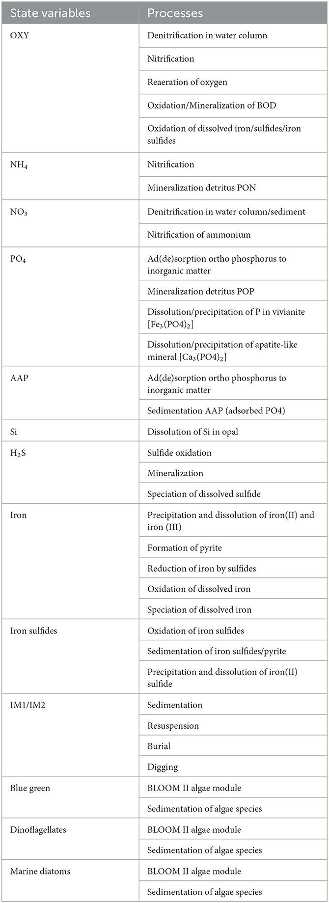
Table 1. Summary of substances and processes activated in the Delft3D-WAQ module.

Detailed descriptions of the formulations relevant to the critical processes for each state variable shown in Table 1 were discussed in the author's dissertation (Lee, 2021) and were derived from the technical reference manual of the Delft3D-WAQ module (Deltares, 2014). In this paper, equations utilized to characterize sediment settling/resuspension and the total bed shear stress are further discussed.

2.3.2.1. Expressions for sediment settling and resuspension

All particulates ranging from several microns to larger than 2 mm are subject to settling and resuspension to and from the bed. Among these, fine-grained particulates sediments, e.g., sand, silt, clay, and organic particles (several to ~70 microns), have high adsorbing capacities and are easily brought into suspension. Thus, the fate and transport of the so-called cohesive sediments heavily influence water quality.

In the DELWAQ module, sediment layers were modeled using the “two layers: S1 and S2 approach.” The sediment layers are subject to resuspension, burial, and digging processes; sediment components are released into the water column by resuspension (erosion) activity (S1 and/or S2), transported to deeper layer (S1 to S2), or removal to even deeper sediment (S2 to the boundary) by burial activity, and lastly, digging transports sediment components from boundary to S2, and from layer S2 to S1. The Partheniades-Krone concept is the principle theory used to express the sedimentation and erosion processes in which the bottom shear stress significantly determines the concentration of suspended sediments in the water column (Krone, 1962; Partheniades, 1962). In this study, the critical shear stress reported by Chung et al. (2009b) was assumed to be the universal critical shear stress for each type of particulate matter and for both modeled layers.

2.3.2.1.1. Sediment settling

Inorganic matter, organic detritus, and algae biomass are subject to settling, and the settled substances become the inorganic sediment pool and part of sediment oxygen demand. The sedimentation process was characterized based on the formulation by Krone (1962) as given in Equation 1:

$\begin{array}{ll}D=w_s·c·\left(1-\frac{{\tau }_b}{{\tau }_c}\right)& (1)\end{array}$

with:

D settling flux of suspended matter (g m⁻² d⁻¹);

w_s settling velocity of suspended matter (m d⁻¹);

c concentration of suspended matter near the bed (g m⁻³);

τ_b bottom shear stress (Pa);

τ_c critical shear stress (Pa).

The sedimentation would occur when the shear stress does not exceed the user-defined critical shear stress and is determined by the products of the near-bed settling velocity of each substance, the concentration, and the probability of settling determined by the ratio of total bottom shear stress and the critical shear stress.

2.3.2.1.2. Resuspension

The resuspension is directly proportional to the excess of the total bed shear stress over the critical bottom shear stress and is described with the formulation by Partheniades (1962) in Equation 2:

$\begin{array}{ll}E=M·\left(\frac{{\tau }_b}{{\tau }_c}-1\right)& (2)\end{array}$

with:

E resuspension flux (g m⁻² d⁻¹);

M first order resuspension rate (g m⁻² d⁻¹);

τ_b bottom shear stress (Pa);

τ_c critical shear stress (Pa).

Resuspension occurs when the actual total bottom shear stress is higher than the critical shear stress for resuspension. The resuspension rate of the individual particulate fractions in the dry sediment matter is proportional to its weight fraction. It is assumed that the upper layer (S1) mass would be completely resuspended before the lower layer (S2) comes in contact with bottom shear stress. Thus, resuspension from the second layer (S2) only occurs if no mass is available in the upper layer (S1). Refer to Lee (2021) and the technical reference manual of the Delft3D-WAQ module for a detailed description of the computations and constraints of the settling/erosion process implementation in Delft3D-WAQ (Deltares, 2014).

2.3.2.2. Expression for total bed shear stresses

The value of the total bed shear stress, along with the critical shear stress, determines the sedimentation and resuspension rates. The shear stresses created by flow (currents) and the wind- generated surface waves, and are additive as follows in Delft3D-WAQ:

$\begin{array}{ll}\tau ={\tau }_{flow}+{\tau }_{wave}& (3)\end{array}$

Nonetheless, the bed shear stress resulting from the combined effects of waves and current surpasses the value obtained through simple linear addition of the bed shear stress due to waves and that caused by the current. Therefore, Delft3D-FLOW provides various wave-current interaction models to express the non-linear interaction at the bed boundary layers enhanced by both waves and current, differentiating between 2D and 3D modeling. The computed total bed shear stress was derived from Delft3D-FLOW and utilized as input parameters in Delft3D-WAQ (Deltares, 2020).

In 3D implementation the bottom boundary layer is consisted of total or effective wave-current combined bed shear-stress, and is corrected for the Stokes drift (i.e. the wave-induced drift velocity) as shown in Equation 4:

$\begin{array}{ll}{\vec{\tau }}_b=\frac{\left|\overrightarrow{{\tau }_m}\right|}{\left|\overrightarrow{U_{2D}}\right|}(\vec{u}-{\vec{u}}^s)& (4)\end{array}$

where $\left|\overrightarrow{{\tau }_m}\right|$ denotes the magnitude of mean bed stress for combined waves and current, and the magnitude of the depth-averaged horizontal velocity, $\left|\overrightarrow{U_{2D}}\right|$, is given by:

$\begin{array}{ll}{\vec{U}}_{2D}=\frac{1}{d+\zeta }{\displaystyle {\int }_{-d}^{\zeta }}\vec{u}dz& (5)\end{array}$

where u is horizontal velocity, (d+ ζ) is total water depth, and z is vertical coordinate.

The mean bed stress for combined waves and current is defined as:

$\begin{array}{ll}{\vec{\tau }}_m={\rho }_0{\overrightarrow{ũ}}_{{}^{*}}\left|{\overrightarrow{ũ}}_{{}^{*}}\right|& (6)\end{array}$

where ρ₀ is density of water, $\stackrel{⃗}{\widetilde{u_{{}^{*}}}}$ is friction (shear-stress) velocity due to current and waves, and can be expressed in the magnitude of the horizontal velocity in the first layer just above the bed ($\overrightarrow{u_b}$) in the logarithmic boundary layer, user-defined bed roughness height (z₀) and constant of Von Kármán (κ= 0.4) as shown in Equation 7:

$\begin{array}{ll}{\vec{u}}_b=\frac{{\overrightarrow{ũ}}_{{}^{*}}}{\kappa }ln\left(1+\frac{\Delta z_b}{2z_0}\right)& (7)\end{array}$

in which z₀ is where the bottom is positioned at in the numerical implementation of the logarithmic law of the wall for a rough bottom and Δz_b is the distance to the computational grid point closest to the bed.

3. Results

3.1. Data inputs and sources

The substances that are subject to sedimentation, including inorganic matter, organic detritus, and algae biomass, constitute the total concentration of sediment. Delft3D-WAQ requires the input of nutrient concentrations to compute the organic nutrient composition of particulate detritus and biomass components of live algae in the sediment. The measured data of water quality constituent concentrations were obtained from the quarterly monitoring program by Bureau of Reclamation in collaboration with the California Department of Water Resources and Salton Sea Authority since 1999. In this study, the calibration period was set between 8/15/2005–9/1/2005, and the sampling dates closest to the calibration period were from June 21 and September 27. Therefore, relevant constituents were derived from the data average between June and September 2005 (Table 2). Since the measured inorganic matter concentrations in the surface and bottom of the Salton Sea in June and September were large in range (20 to 144 mg/L), the mode value (~54 mg/L) was selected to carry out the calibration/validation tests. IM1 denotes the fine inorganic matter fraction, and IM2 represents the fraction of the coarse fraction. Those marked “modeled” specified the substances whose values were derived from water quality processes in the model.

TABLE 2

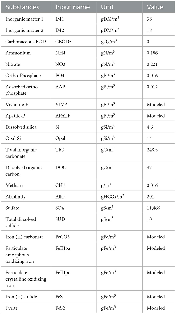
Table 2. Summary of input substance values for Delft3D-WAQ used for suspended sediment calibration/validation tests.

The latest measured suspended sediment concentration data were collected by Chung et al. (2009b) during a field measurement program from 8/2/2005 to 11/25/2005. The measured turbidity concentrations (a surrogate for suspended sediment concentration) were collected by optical backscatter sensors (OBSs) that were deployed 0.5 m off the bottom of the water depths of 4, 6, and 8 min the southeastern basin of the Salton Sea (Chung et al., 2009b).

Sensitivity tests were conducted to evaluate various parameters' effects on suspended sediment concentrations. The parameters for sensitivity tests in suspended sedimentation simulation include sedimentation velocity IM1/IM2, zeroth-order resuspension flux, and first-order resuspension flux. The evaluation results suggested that among zeroth-order resuspension flux (ZResDM), first-order resuspension flux (VResDM), zeroth-order digging flux (ZDigDM), first-order burial velocities (VBurDM), and sedimentation velocities, the parameters of VResDM, VBurDM, and Settling velocities play significant roles in determining the level of sediment resuspension events in the water column (data not shown).

Based on the sensitivity tests, process parameters most relevant to sediment solids sedimentation and resuspension are summarized in Table 3. The sedimentation velocities of settling matters ranged from 0.2 to 1 m/d, and the algae sedimentation velocities were the default values.

TABLE 3

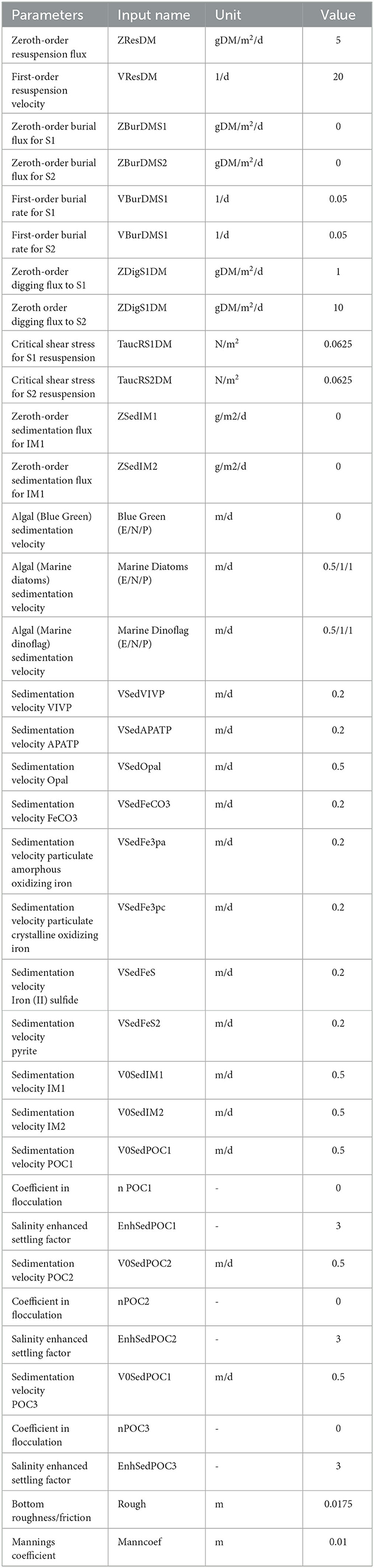
Table 3. Summary of process parameter values for Delft3D-WAQ used for suspended sediment calibration/validation tests.

3.2. Model validations

3.2.1. Sediment concentration and bottom shear stress validation

The warm-up period for the calibration task was from 8/8/2005 00:00:00 to 8/15/2005 00:00:00. The last timestep in the restart file of the warm-up run was used as the initial conditions for the calibration runs. The simulated suspended solid concentrations in the water column at the southeastern basin were calibrated against the measured turbidity data from 8/15/2005 to 9/1/2005 at roughly the same location where the OBS was placed based on the study by Chung et al. (2009b). The validation period was from 9/1/2005 00:00:00 to 9/17/2005 00:00:00, and the initial condition on 9/1/2005 was derived from the last timestep of the calibration period.

The overlay of simulated total bottom stress and bottom shear stress caused by waves is shown in Figure 2A. The simulated suspended sediments (mg/L) and the measured turbidity (NTU) data are shown in Figure 2B. Note that the relationship between turbidity and total suspended solids was converted by an equation tested previously on Mark Twain Lake (Knowlton and Jones, 1995): TSS(mg/L) = 0.932 × TURB(NTU)+0.0038 × TURB². The conversion results in a roughly 1:1 ratio between turbidity (NTU) and suspended solids concentration (mg/L).

FIGURE 2

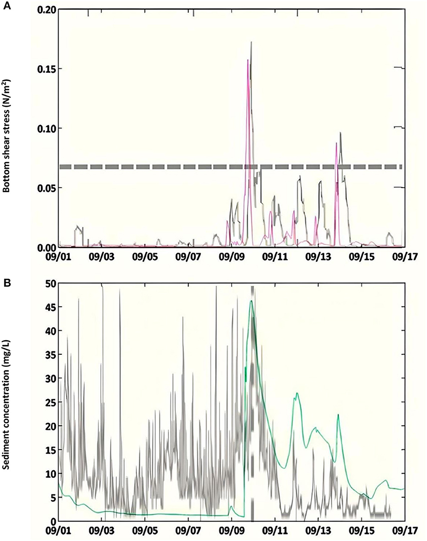
Figure 2. Comparison of bottom shear stresses (A) and suspended solid concentrations (B) from the validation period, 9/1/2005 to 9/17/2005, at 0.5 m off the bottom at a depth of 6 m. The measured data was shown in the black line, the simulated bottom shear stress was demonstrated in the pink line, and the simulated sediment concentration was shown in the green line. Figures adapted from Chung et al. (2009a). Copyright 2009 by the American Geophysical Union.

Correlation between TSS and turbidity is convenient because turbidity is easily measured. This type of correlation has been used before and has been shown to be affected by particle size distribution. Generally, the smaller particles contribute more to turbidity than larger particles. Ferreira and Stenstrom (2013) have evaluated particle size distributions and correlations to TSS. Particle size is always a more desirable parameter but is more difficult to measure and generally not available in the published literature (Ferreira and Stenstrom, 2013). Li et al. (2006) has discussed particle size distribution and turbidity and their work can be consulted for more information and limitations.

The simulation results of the sediment concentration in the water column showed a strong correlation with the bottom shear stress. In Figure 2A, the horizontal gray dash line indicated the critical shear stress of 0.0625 N/m² (calculated based on the sediment size of 25 μm) reported in Chung's study, and the result showed that the simulated bottom shear stress matched with the measured shear stress caused by waves reasonably well. The bottom shear stress increased significantly and reached 0.17 N/m² on 9/9/2005 at 18:00 when the storm occurred and remained at the average level of critical shear stress during the storm period.

The data showed that the bottom shear stress from 9/1/2005 to 9/9/2005 was mostly below 0.01 N/m². As a result, the solid sediment concentration remained low at 5 mg/L before the storm occurred. As the bottom shear stress increased due to strong waves when the storm started, the model resolved a significant increase of the simulated sediment solid concentrations from 5 to 45 mg/L that matched the level of the measured data well (Figure 2B).

Overall, the assessments suggested that the validated model could generate suspended sediment concentration in the water depth of about 5.5 m (0.5 m off from the bottom near south eastern shore) at a reasonable range compared to the values taken at the same water depth and location. In addition, the timing of sediment resuspension in the water column corresponded with the simulated bottom shear stress and matched well with the observed data.

3.2.2. Water quality variables validations

The water quality parameters selected for the water quality validation test were dissolved oxygen (DO), unionized ammonia (NH₃), orthophosphate (PO₄), and chlorophyll a. In the WAQ module, the period to generate initial conditions was from 8/8/2005 to 8/15/2005, followed by a calibration period from 8/15/2005 to 9/1/2005, and nearly 2 years of validation period from 9/1/2005 to 8/8/2007. The validated model output for DO was compared with the measured values in Figure 3.

FIGURE 3

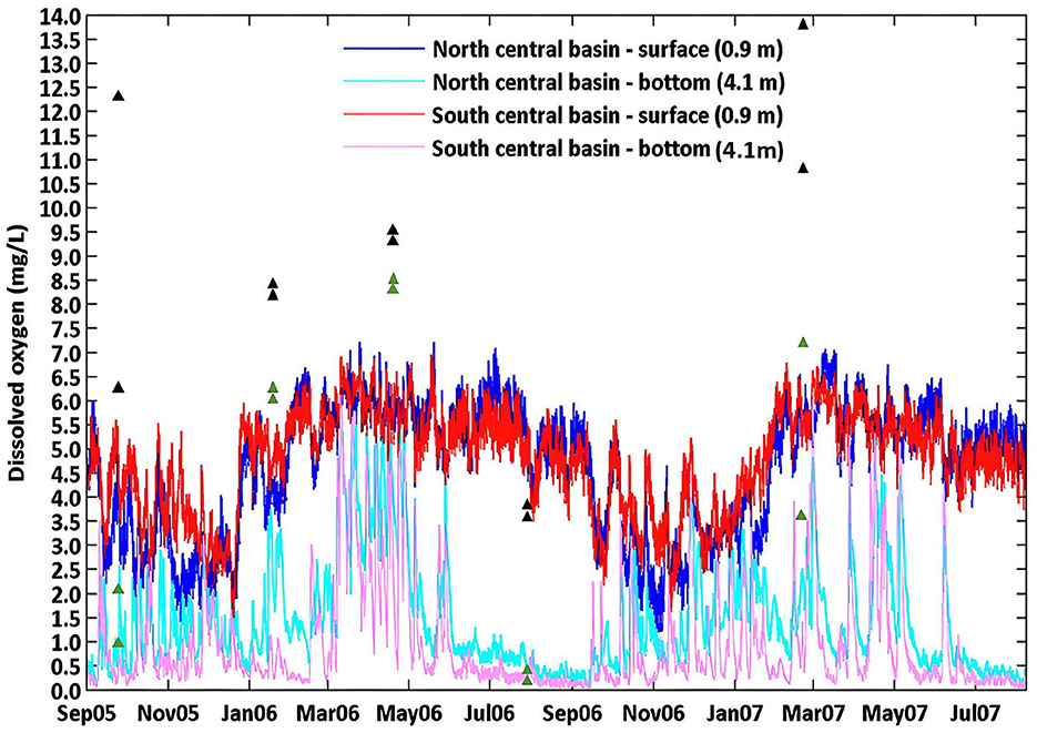
Figure 3. Comparison between the measured DO (triangles) and the simulated DO (lines) in north central/south central basins of the Salton Sea at 0.9 m from the surface and 4.1 m above the bottom from 9/1/2005 to 8/8/2007. The black triangles denote measured data at 0.95 m from the surface, and green triangles denote that from 4.1 m above the bottom.

A more detailed schematization is required in the FLOW module for hydrodynamics modeling than water quality simulation, but it not only would take more computational time than is necessary, it may cause computational bias in water quality constituents' calculations, especially those parameters that are sensitive to water depths such as oxygen. Therefore, vertical aggregation in the WAQ module played a significant role in determining the values of the water quality parameters. The vertical grid was aggregated from 16 layers in the FLOW module into six layers in the WAQ module. In this work, an σ-grid (constant number of layers, with varying layer thickness) was used for 3D computation. The aggregated layer thickness from top to bottom is 6.8, 6.8, 10.05, 18, 27, and 30.9%, which is equivalent to dynamic segment depths of 0.95 m, 0.95 m, 1.47 m, 2.52 m, 3.78 m, 4.1 m, respectively in roughly central north and south basin regions.

Figure 3 shows that DO concentrations in 0.95 m below the surface were generally underestimated except in July. The WAQ module could not compute DO concentration in a segment smaller than 0.95 m within the surface layer. As a result, the higher reaeration rate and gross primary algal production rate that occurred at the surface level were not accounted for in the WAQ module. On the other hand, the DO concentration in the bottom layer matched the measured values fairly well, with a small level of underestimation during the spring season.

The validated model output for NH₃ was compared with the measured values in Figure 4. At a constant pH value of 8.2, the results showed that simulated results from the central south basin are in better agreement with the measured values among the two basins.

FIGURE 4

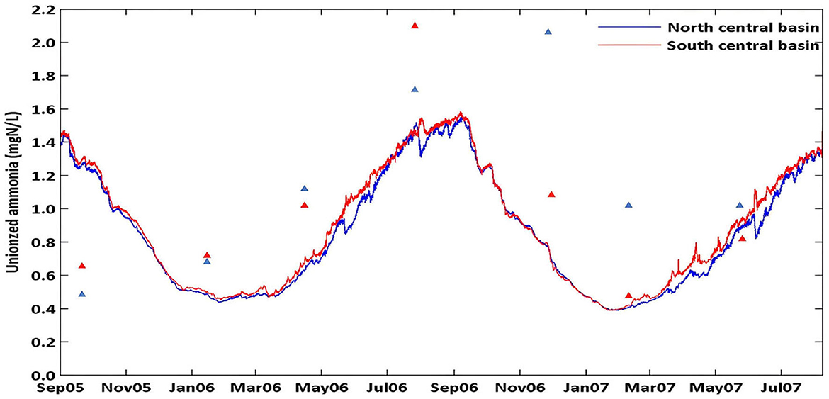
Figure 4. Comparison between the measured unionized ammonia (triangles) and the simulated depth-averaged unionized ammonia (lines) in the Salton Sea's north central/south central basins from the validation period, 9/1/2005 to 8/8/2007. The blue triangles denote measured depth-averaged values in the north central basin, and the red triangles denote that in the south central basin.

Note that the input nutrient concentrations (ammonium, nitrate, and orthophosphate) at the river discharge locations were set at constant values using the average of the quarterly data from September 2005 to May 2007 due to the lack of daily measurements. Therefore, the variability in nutrient inputs was not fully captured. Nonetheless, the WAQ module successfully resolved the seasonal fluctuations of unionized ammonia. Unionized ammonia concentrations were within a 24% difference in the south-central basin and a 66% difference in the north-central basin compared to the observed values.

The validated model output for orthophosphate was compared with the measured values in Figure 5. The simulated results showed an over-prediction before winter 2007 and an under-prediction in February 2007 but were overall in the close range of the measured values. The discrepancy could result from lacking several factors needed in the processes for the mass balance equations.

FIGURE 5

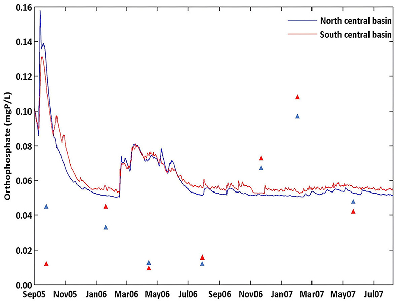
Figure 5. Comparison between the measured orthophosphate (triangle) and the simulated depth-averaged orthophosphate (lines) in north central/south central basins of the Salton Sea from the validation period, 9/1/2005 to 8/8/2007. The blue triangles denote measured depth-averaged values in the north central basin, and the red triangles denote that in the south central basin.

The WAQ module computes dissolved orthophosphate based on the mass balance as given in Equation 8:

$\begin{array}{l}\frac{\Delta P{O}_4}{\Delta t}=loads+transport\pm sorption+mineralization\\ \pm precipitation+primaryproduction+autolysis\\ +atmosphericdeposition\pm sedimentexchangeflux& (8)\end{array}$

Among these, the process of phosphorus adsorption onto suspended sediments and precipitation/dissolution of vivianite and apatite minerals were subjected to huge uncertainty due to lacking information on the iron-containing fraction of the sediments and iron (II) concentrations in the Sea, as well as the fractions of nutrients are released into the water column when primary producers die in the autolysis process. Default values were used to replace the unknown parameters in the WAQ simulation.

The two peaks of PO₄ concentrations in September 2005 and March 2006 resulted from sediment resuspension-induced orthophosphate desorption in the water column. The two peak events were the direct results of the two storm events that occurred during that time. Note that the WAQ module assumes that phosphate desorption and mineralization fluxes from the sediment layers are instantaneous inputs to the entire water column, leading to peaks of high orthophosphate concentrations in the water column, as shown in Figure 5. However, the observed values were usually measured in calm weather. Overall, the simulated results showed that the resuspension flux of adsorbed phosphate from the sediments is the main driving force in determining the orthophosphate concentrations in the water column.

3.3. Water quality mitigation strategies simulations

Previous studies have repeatedly confirmed that sediment resuspension plays a significant role in influencing the water quality of the Salton Sea, and winds heavily drive the resuspension events. Therefore, in this study, the scenario of using emerged islands to serve as a wind fetch obstruction device was simulated. It is a water quality mitigation strategy targeting the important wind-induced sediment resuspension mechanism in the Salton Sea.

The Salton Sea's other critical water quality issue is the rising salinity. The second mitigation scenario, seawater import/export implementation, was simulated to assess the impacts on salinity and consequential water quality dynamics in the Salton Sea. Lastly, the combination of seawater canals and treated tributary inflows was simulated as the most robust mitigation strategy. The nutrients (ammonium-N, nitrate/nitrite-N, and orthophosphate) in the treated tributary river water were reduced by 90% before entering the Sea. The timeframe of simulations for the status quo condition and the three mitigation scenarios was from 8/8/2005 to 8/8/2007. Within the time frame, the calibration period in the FLOW module is from 8/8/2005 to 9/1/2005, and the validation period is from 9/1/2005 to 8/8/2007. In the WAQ module, the period to generate initial conditions is from 8/8/2005 to 8/15/2005, followed by a calibration period from 8/15/2005 to 9/1/2005, and the nearly 2 years of validation period from 9/1/2005 to 8/8/2007.

3.3.1. Status quo

In the status quo condition, the Sea is at its original state and configuration without any additional infrastructures and modifications.

3.3.1.1. Water temperature

In the center of the north basin, where the deepest water depth reaches 83 m below sea level, the simulation results showed a distinct thermal stratification before the storm occurred in the evening of 9/9/2005, ranging from 29 to 34°C. The temperature range of 29 to 30°C and 33 to 34°C dominated the bottom and surface three to four meters in depth. Diurnal temperature fluctuations in the surface layer were resolved by the model, represented by the intermittent one degree, sometimes up to two degrees increase in the surface layer. During the storm period from 9/9/2005 to 9/15/2005 (marked by the red brackets), it was shown that the water temperature became homogeneous throughout the water column, averaging the surface and bottom temperature and keeping the water temperature at the range of 30 to 32°C. Later on, the water column remained homogenous in temperature as it entered fall season (Figure 6A).

FIGURE 6

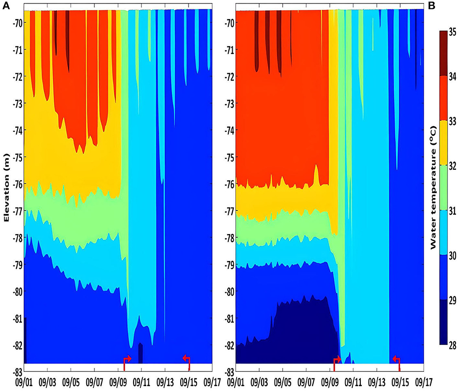
Figure 6. Simulated thermal stratifications in (A) central north and (B) central south basin from 9/1/2005 to 9/17/2005 in the status quo condition. The red bracket denotes the storm period.

During the same period, the thermal stratification in the center of the south basin showed a larger temperature stratification from 28 to 35°C from the bottom to the water surface before the storm events (Figure 6B). However, compared to that of the north basin, almost the entire six meters down from the surface were constant in the range of 33 to 34°C, with an occasional increase to 35°C. A less structured thermocline was shown in the central south basin where most of the water column was 33 to 34°C, followed by rather sharp transitional layers from −77 to −79.5 m in depth where the temperature dropped three degrees to reach the range of 28 to 30°C from three meters above the bottom. During the storm period, a homogeneous temperature range of 30 to 31°C also occurred dominantly in the south-central basin, followed by a homogeneous temperature range of 29 to 30°C in the fall season. The results were consistent with the findings presented by Rueda et al. (2009), in which a more prominent thermal stratification was shown in the north basin, and a less structured thermal stratification was in the south basin.

3.3.1.2. Horizontal velocity

Time-series (9/1/2005 00:00:00 to 9/17/2005 00:00:00) of horizontal velocity magnitudes in the north and south basin center are shown in Figure 7. The simulation showed that during the peak of the storm event on 9/9/2005 at 18:00, the horizontal velocity magnitude increased from about 0.03 m/s to 0.3 m/s in both basins from two meters above the bottom. However, during the storm period, the simulation showed slightly higher velocity (< 0.03 m/s higher) in the northern basin. This phenomenon could be due to the fact that the deepest depth of the north basin was about one meter deeper than that of the deepest depth of the south basin, and the south basin is generally shallower.

FIGURE 7

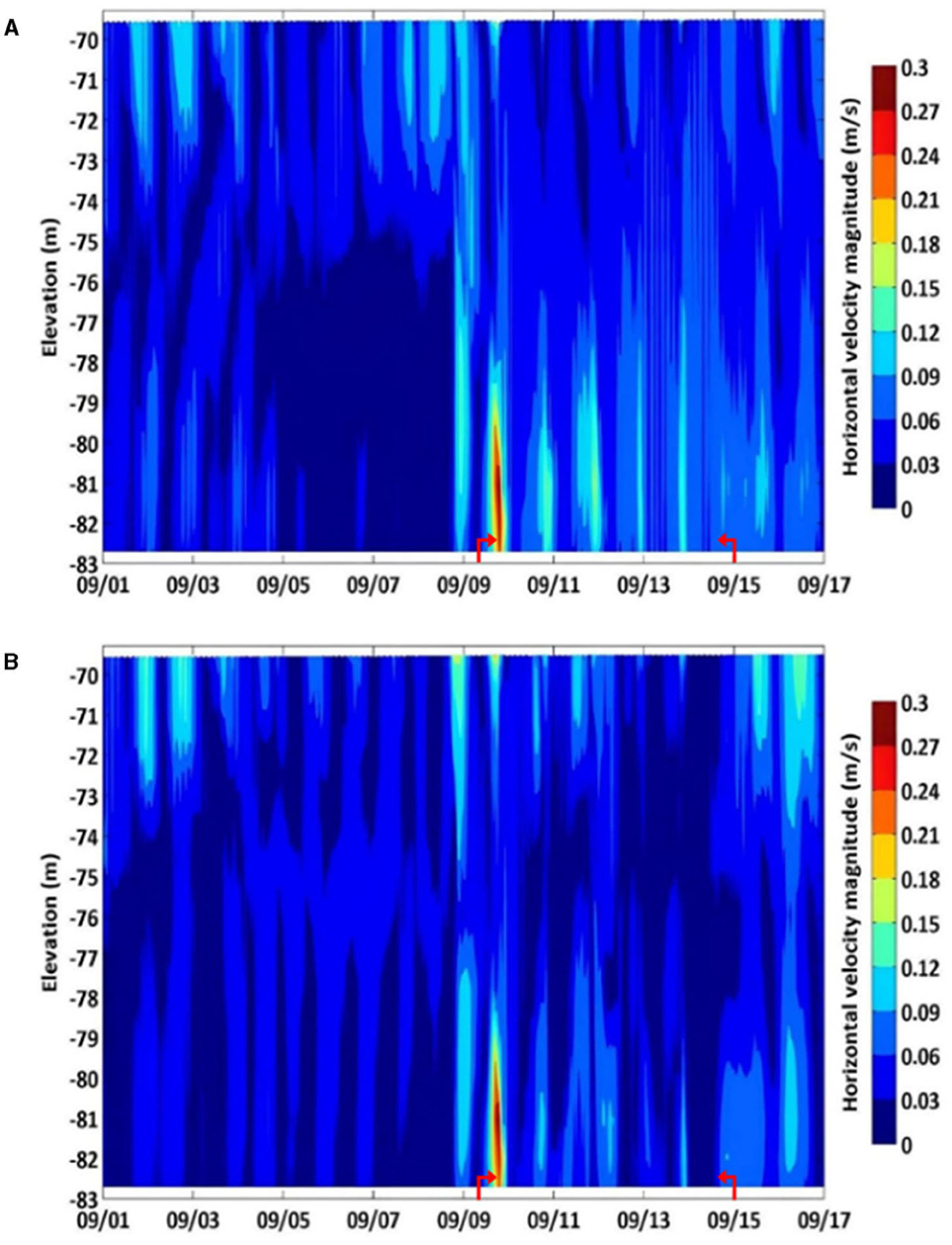
Figure 7. Simulated horizontal velocity magnitudes in depth contour in central north (A) and central south basin (B) from 9/1/2005 to 9/17/2005 in the status quo condition. The red bracket denotes the storm period.

3.3.2. Emerged islands as wind obstruction device scenario

The wind speed and direction from 8/1/2005 to 9/27/2005 measured at the southeastern meteorological site CIMIS #128 showed that the predominant wind direction was from northwest, southeast, and southwest directions, among which wind blowing from 240° to 270° was especially stronger than the rest of the direction. As a result, the emerged islands that obstruct wind fetch and interfere with the flow from the two main tributary rivers from the south end were designed to block the predominant wind patterns. The emerged islands consisted of five rigid sheets extended from the bottom to above the surface of the Sea with surface areas ranging from 2 to 2.5 mi² in the south basin of the Sea.

3.3.2.1. Water temperature

The thermal stratification simulation results in the presence of the emerged islands suggested that having installed islands in the south basin would minimally affect the thermal stratification structure in the north basin compared to the status quo condition. The thermal stratification in the north central basin during the same timeframe was almost identical to that in the status quo (Figure 8A). Similarly, the central south basin also showed similar thermal stratification compared to the status quo where a deeper layer of the temperature range (33 to 34°C, with occasional 35°C) was extended from the surface to six meters below the surface, followed by a steep temperature drop from 33 to 30°C from −76 to −79 m msl (Figure 8B).

FIGURE 8

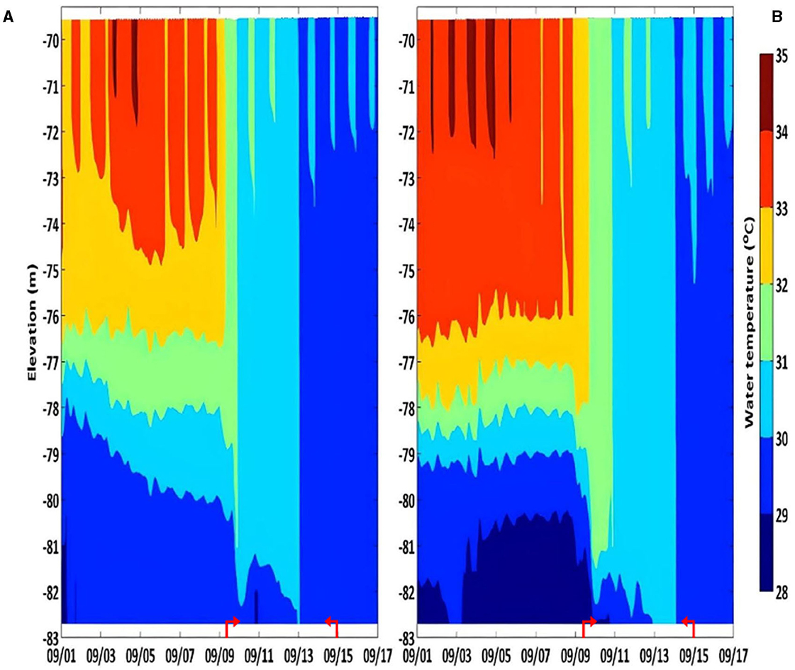
Figure 8. Simulated thermal stratifications in central north (A) and central south basin (B) from 9/1/2005 to 9/17/2005 in the presence of emerged islands. The red bracket denotes the storm period.

However, the change occurred in the central south basin during the storm period, where it appeared that the water column was not completely homogenous in temperature; the water column showed a larger temperature range of 29 to 32°C compared to 30 to 31^oC in the status quo condition. The low temperature only occurred from 1.5 meters above the bottom. This phenomenon suggested that the emerged islands prevented the water column from being completely mixed in the central south basin (Figure 8B).

3.3.2.2. Horizontal velocity

Compared to the horizontal velocity magnitudes in the status quo, the simulation results in the presence of emerged island showed that the central north basin also experienced the same degree of higher horizontal velocity during the storm period at 5 meters above the bottom; the velocity increased up to 0.27 m/s during the storm peak, and to 0.15 m/s on average during the storm period (Figure 9A).

FIGURE 9

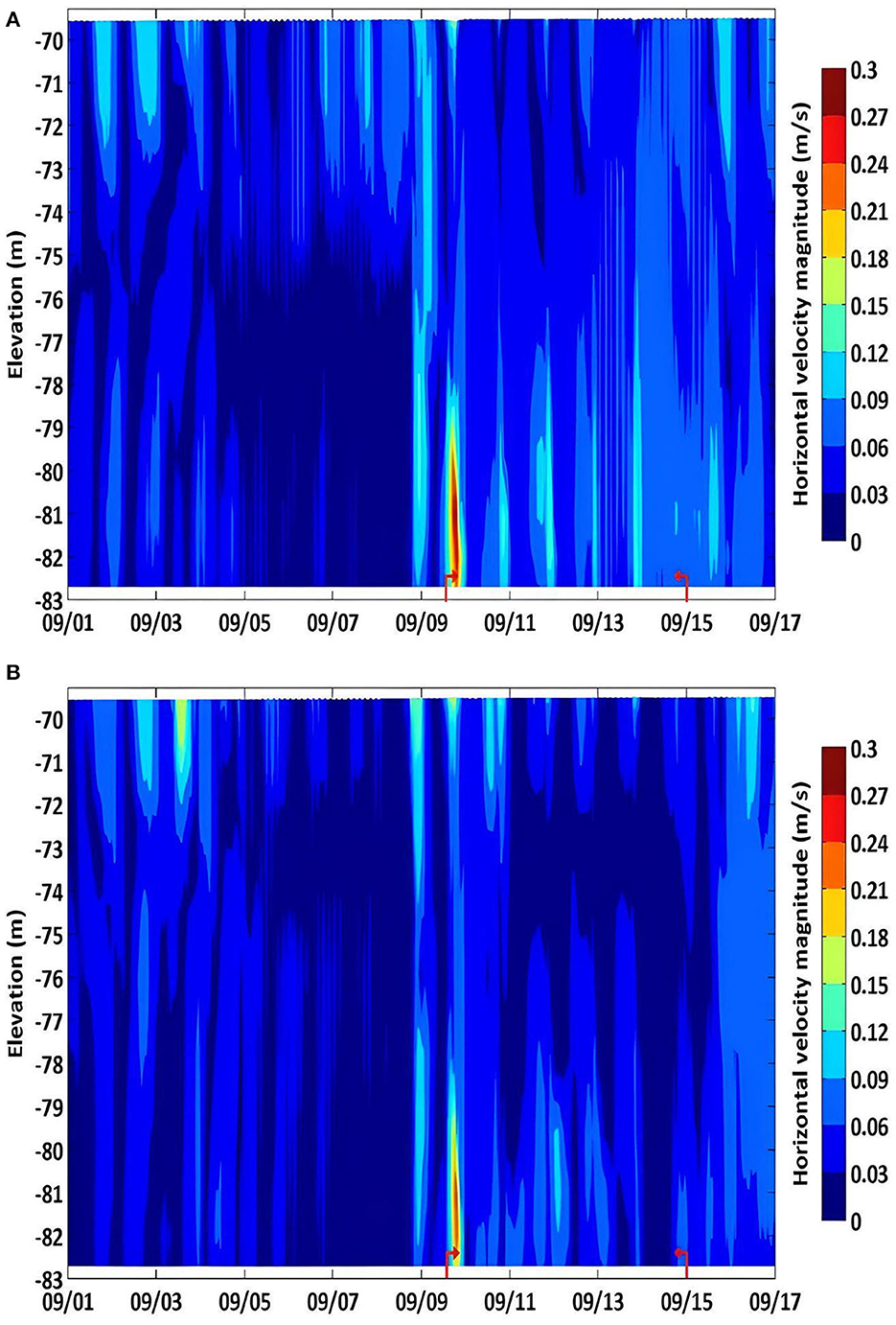
Figure 9. Simulated horizontal velocity magnitudes in depth contour in the central north basin (A) and central south basin (B) from 9/1/2005 to 9/17/2005 in the presence of emerged islands. The red bracket denotes the storm period.

On the contrary, during the storm peak, the horizontal velocity magnitude in the central south basin decreased to the range of 0.21 to 0.24 m/s, which was up to a 0.06 m/s decrease compared to that in the status quo. The results showed that reduced wind fetch effectively reduced horizontal velocity toward the bottom of the central south basin (Figure 9B).

3.3.3. Seawater import/export scenario

Canals have been suggested as a way of reducing the salinity of the Salton Sea. To evaluate this option, seawater import and export was simulated. The seawater import and export canals locations are in the south and north shorelines, respectively.

A first-order integration of a continuous stirred-tank reactor model was utilized to estimate the seawater inflow/outflow rates. The mass balance to estimate out-going salinity was calculated as given in Equation 9:

$\begin{array}{ll}V\frac{dC}{dt}=Q_{in}·C_{in}-Q_{out}·C_{out}& (9)\end{array}$

where V denotes the volume (m³) of the Sea using an average depth of 9 m, and C_in, C_out represent salinity concentration in the unit of g/m³, t is timestep in second, and Q_in, Q_out denote the canals flow rates (m³/s) at inflow and outflow, respectively.

The components of inflow/outflow flow rates and concentrations were described as given in Equations 10–12:

$\begin{array}{ll}{Q}_{in}=Q_{in,sea}+Q_{in,newriver}+Q_{in,alamoriver}& (10)\end{array}$

$\begin{array}{ll}{Q}_{out}=Q_{out,sea}+Q_{out,evaporation}& (11)\end{array}$

$\begin{array}{ll}{C}_{in}=C_{in,sea}+C_{in,newriver}+C_{in,alamoriver}& (12)\end{array}$

Average values for the tributary river flows and evaporation rates were used to estimate the out-going salinity concentration.

Based on the estimation, the salinity would gradually decrease from 46 ppt in 2005 and be stabilized at around 38 ppt in 2.47 years. The current salinity of the Salton Sea is approximately 74 ppt, and it would take about 4.5 years for the salinity to drop and stabilize at the level of 38 ppt.

3.4. Water quality simulations in the status quo and mitigation scenarios

The long-term effects on Salton Sea's water quality in the status quo and three water quality mitigation strategies: (1) the presence of emerged islands, (2) having seawater imported/exported into/out of the Sea, and (3) combining seawater canals implementation with treated tributary rivers scenarios (90% nutrients reduction) were simulated in this study. A water quality simulation of ~2 years from 9/1/2005 to 8/8/2007 is shown in this section, and the water quality variables being examined are dissolved oxygen (DO), orthophosphate (PO4), unionized ammonia (NH3), chlorophyll a (Chl a), and salinity.

3.4.1. Dissolved oxygen

Mean dissolved oxygen concentrations in the 0.95 meters below the surface and 4.1 meters above the bottom of the Sea in four scenarios during the summer season (4/1/2007–6/30/2007) are shown in Figure 10. The simulation showed that in the status quo condition, the mean DO concentration was approximately 5 mg/L (90% of saturation) in the first meter below the surface (Figure 10A1) and dropped below 2 mg/L from the bottom to roughly four meters above the bottom (Figure 10A2).

FIGURE 10

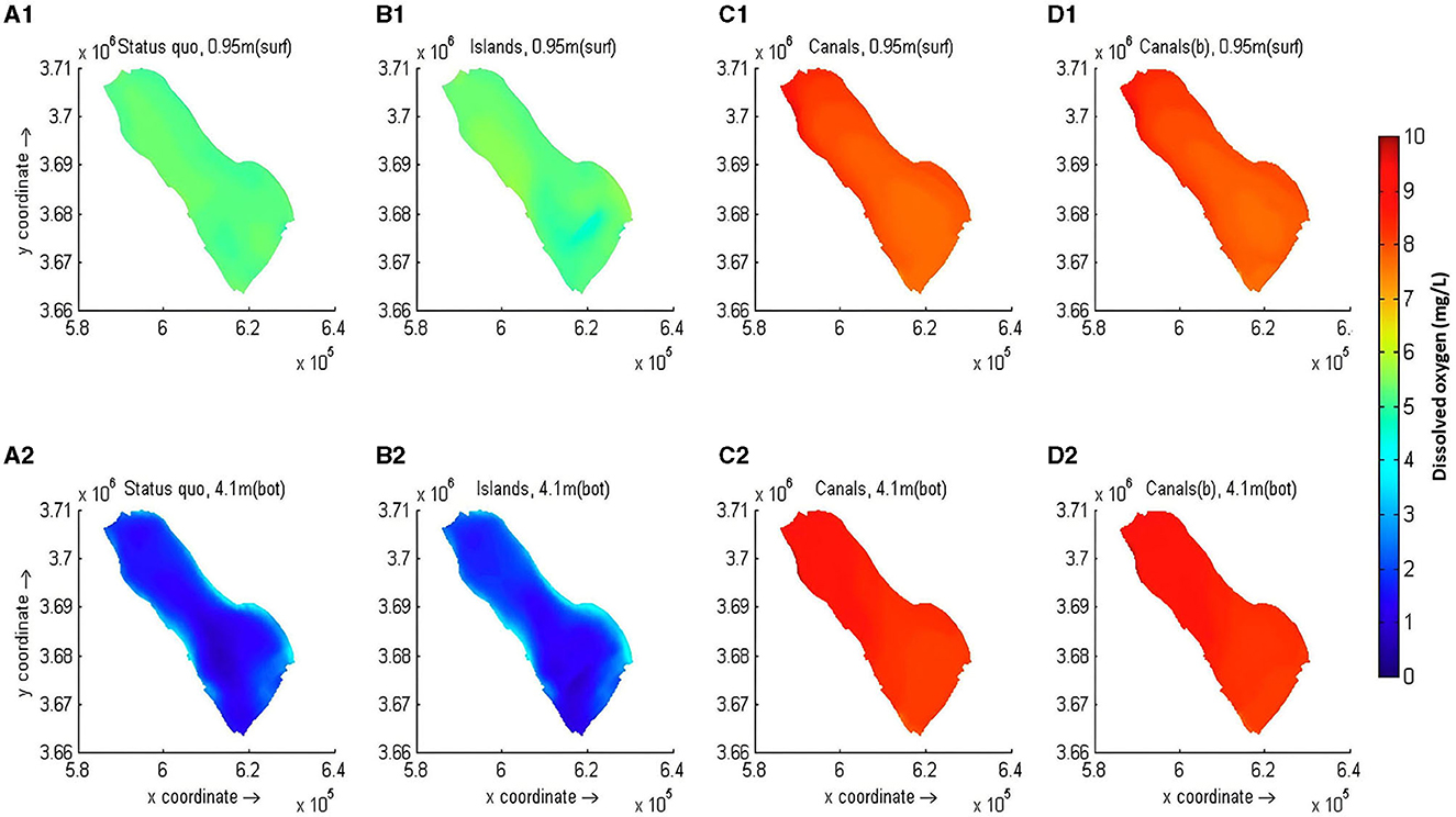
Figure 10. Comparison of the simulated mean dissolved oxygen (DO) concentrations in the status quo condition (A1, A2) and under the three mitigation scenarios, including emerged islands (B1, B2), seawater canals (C1, C2), and seawater canals with treated tributary rivers (D1, D2) during simulated period, 4/1/2007 to 6/30/2007. The upper four figures represent DO concentrations at 0.95 m below the surface, and the lower four figures show that of 4.1 meters above the bottom.

In the presence of emerged islands, the DO concentration in the top 0.95 meters of the surface showed similar results to the status quo but about 0.5 mg/L higher in the bottom layer (Figures 10B1, B2). For the canal option, high DO saturated water (8 mg/L) was imported into the Salton Sea at the rate of 225 m³/s in the south basin, and the lake water in the north basin was exported at 215.5 m³/s from layer 5 in the seawater import/export scenario (Figures 10C1, C2). As a result, the DO concentration in the surface layer increased to 8 to 9 mg/L, and in the bottom four meters, the DO concentrations increased to approximately 8 to 10 mg/L on average during spring 2007. The reason why the DO level in the bottom layer showed approximately 1 mg/L higher than the surface layer is due to the general underestimation of the surface layer discussed in the previous section. Lastly, treated tributary inflows combined with seawater canals implementation showed rather similar results to the canals-only scenarios (Figures 10D1, D2).

3.4.2. Orthophosphate

The results of depth-averaged PO₄ concentration in the north and south-central basins are shown in Figure 11. In the status quo condition, orthophosphate concentrations peaked in the range of 0.08 to 0.16 mg/L in response to the two storms (>12 m/s) that occurred in the Salton Sea and maintained at approximately 0.058 mg/L in both north and south-central basins during regular days.

FIGURE 11

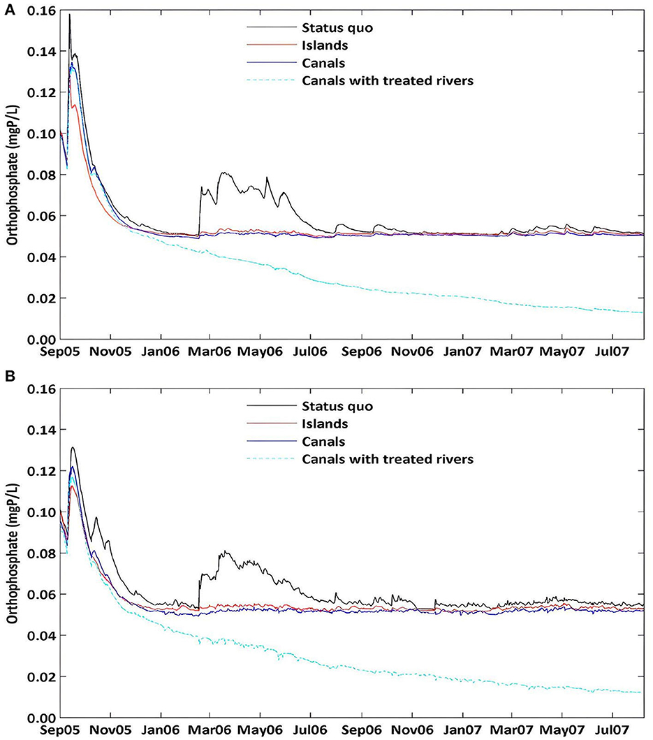
Figure 11. Comparison of the mean simulated orthophosphate concentrations in the status quo condition and under three mitigation scenarios from 9/1/2005 to 8/8/2007 in (A) the north central basin and (B) the south central basin in the Salton Sea.

Orthophosphate adsorbs onto the adsorbing components of suspended sediments including iron(III)oxyhydroxides, aluminum hydroxide, silicates, manganese oxides, and organic matter. The mechanism of PO₄ removal in the scenario of constructing emerged islands is mainly associated with sediment activities. The wind-induced sediment resuspension activities were reduced because of reduced bottom shear stress; hence, less resuspension occurred to release orthophosphate into the water column. The simulation showed that islands reduced PO₄ by 18% during the first storm and 31% in the second storm compared to the status quo.

The seawater import/export scenario brought in seawater that was set to have no PO₄ along with sediments from the south basin at 225 m³/s and exported lake water that contained average PO₄ and sediment concentrations in the north basin at 215.5 m³/s. The results showed that depth-averaged PO₄ concentration in the north-central basin decreased by approximately 14% during the first storm and 36% during the second storm compared to the status quo. In the south-central basin, the peak decreased by 8.3% during the first storm and 36% during the second. After a year of simulation, the decrease percentage remained at approximately 5% in the north-central basin and 8% in the south-central basin from August 2006 till August 2007. Finally, in the scenario where nutrients in the tributary rivers were reduced by 90% in addition to seawater canals implementation, the results showed a drastic decline in PO₄ concentrations starting from March 2006. The level of orthophosphate concentrations was as low as 0.01 mg/L by August 7, 2007, in the Salton Sea's north and south-central basins (Figure 11).

3.4.3. Unionized ammonia

Unionized ammonia is toxic to aquatic life and is contributed mainly by the tributary river inflows that contain municipal wastes and agricultural and manure application runoff. The unionized ammonia is the product of the ammonium (${\text{NH}}_4^{+}$) ion dissociation, which is subjected to aerobic nitrification to produce nitrate (NO₃). Therefore, unionized ammonia's fate depends on the water column's dissolved oxygen level. During the summer, dissolved oxygen decreases due to high water temperature and massive algal production, causing less nitrification and favoring ammonium ion dissociation, eventually accumulating unionized ammonia concentration in the water column. This phenomenon is resolved successfully by the WAQ module; unionized ammonia concentrations had seasonal fluctuation patterns in the status quo and all three other mitigation strategies, as shown in Figure 12.

FIGURE 12

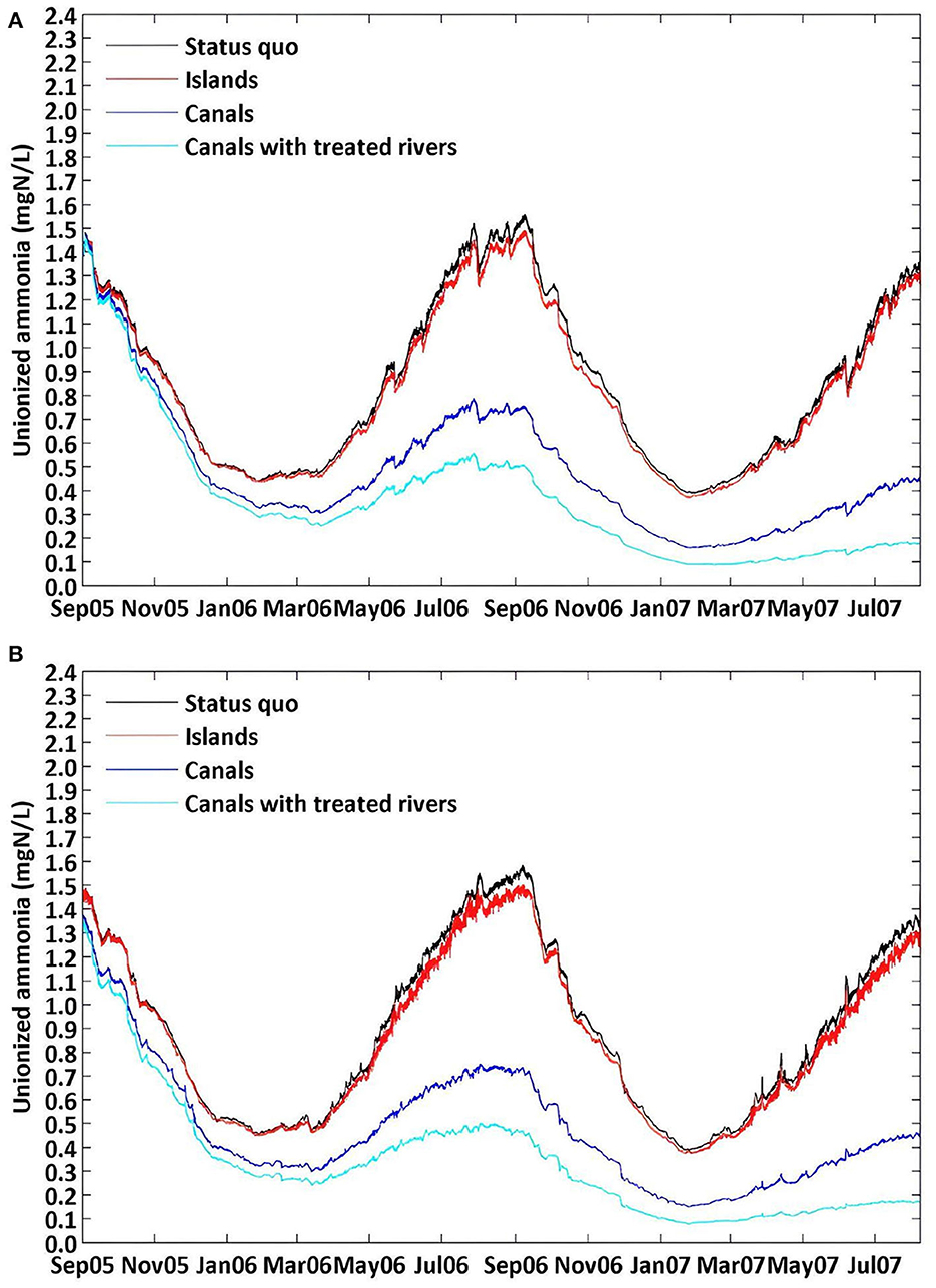
Figure 12. Comparison of the simulated mean unionized ammonia concentrations in the status quo condition and under three mitigation scenarios from 9/1/2005 to 8/8/2007 in (A) the north central basin and (B) the south central basin in the Salton Sea.

The emerged islands in the south basin served to restrict currents loaded with high ammonium concentrations from the New and Alamo Rivers and prevented the inflows from being further transported into the whole sea before being taken up by phytoplankton or undergoing nitrification. The effects of unionized ammonia decline were most prominent during the summer (from June to early September), in which NH₃ decreased to approximately 6.3% in the presence of emerged islands. In the seawater import/export scenario, the imported seawater was set to contain zero ammonium concentration, and an average level of ammonium was being exported out of the Sea. The simulation showed a tremendous decrease in unionized ammonia concentration in the Sea. During summer 2006 when NH₃ concentration peaked, NH₃ decreased by approximately 49.3% in the presence of seawater canals and by 68.3% in the scenario where 90% of nutrients were removed in the tributary rivers in addition to seawater import/export implementation (Figure 12). In the most robust scenario, the simulation showed that the decrease of NH₃ became even larger from June 2007. Nonetheless, after two years of simulation, it was shown that the unionized ammonia level in the Salton Sea was still above the critical level of 0.05 mg/L in all scenarios.

3.4.4. Chlorophyll a

The chlorophyll a concentration in the spring season is highest throughout the year; therefore, the maximum values in the spring season (4/1/2007–6/30/2007) were chosen to represent algal productivity in all four scenarios (Figure 13). In spring 2007, the chlorophyll a concentration in the status quo reached the range of 400–450 μg/L near the central basin, and the concentration in the south basin was up to 1.25 times higher than that in the north basin (Figure 13A). In the presence of islands, it was shown that high algal productivity was localized in the south basin at a lower range of 350–400 μg/L (Figure 13B). The results were expected since main nutrients sources were from the New and Alamo River from the south end, and that the presence of islands interfered nutrients transportation toward northward, therefore lowering algal production in general.

FIGURE 13

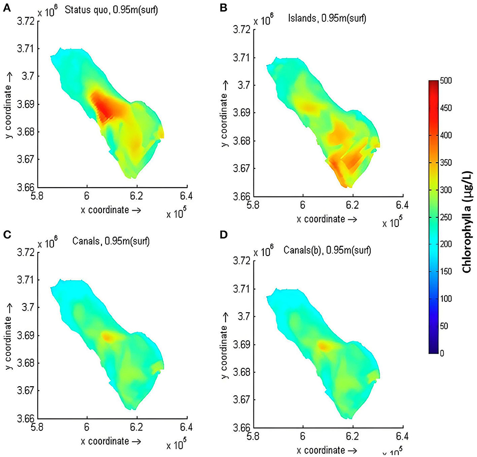
Figure 13. Comparison of the simulated maximum chlorophyll a concentrations in (A) the status quo condition and in mitigation scenarios including (B) islands, (C) seawater canals, and (D) treated tributary inflows with canals from 4/1/2007 to 6/30/2007.

At the end of the 2-year simulation, the level of ammonium in the seawater canals scenario was one-half of that in the status quo, and the nitrate level in the canals scenario was about 36% of that in the status quo (data not shown). As a result, the maximum chlorophyll a concentration during Spring in 2007 in the canal scenarios was lower at the range of 200–300 μg/L with only the central basin having higher Chl a concentration of up to approximately 350 ug/L (Figure 13C).

In the scenario where inflows nutrient concentrations were reduced by 90%, the ammonium, nitrate, and orthophosphate concentrations were 16, 4.5, and 17% of that in the status quo, respectively, by August 2007 (data not shown). Nonetheless, the simulation results showed that the maximum Chl a concentration in Spring 2007 was identical to that in the implementation of the canals without tributary treatment scenario (Figure 13D). The reason is due to the growth constraints within the BLOOM module are set to maximize the total net growth; if the actual biomass is lower than the threshold biomass concentration of an algal species at the beginning of a timestep, threshold (minimum) level would be used. By reducing the timestep from 6 h to 1 h in BLOOM, the algal biomasses between the two canals scenarios started to diverge in June 2007. The alternative simulated results showed that the chlorophyll a concentrations decreased by 9% in the canal scenario with treated inflows in the summer of 2007 (data not shown).

3.4.5. Total bottom shear stress

The total bottom shear stress in the status quo condition and the impact of building emerged islands on the bottom shear stress are compared in Figure 14. The figures present the maximum total bottom shear stress of the whole Sea in September 2005, during which the first storm occurred. Even though the emerged islands consisted of five separate rigid sheets extended from the bottom to above the surface with surface areas ranging from 2 to 2.5 mi², the simulation showed that the general region covered by the emerged islands experienced lower bottom shear stress at the range of 0.02 to 0.04 N/m² (Figure 14B). The effects of reduced wind fetch were also shown near the eastern shorelines.

FIGURE 14

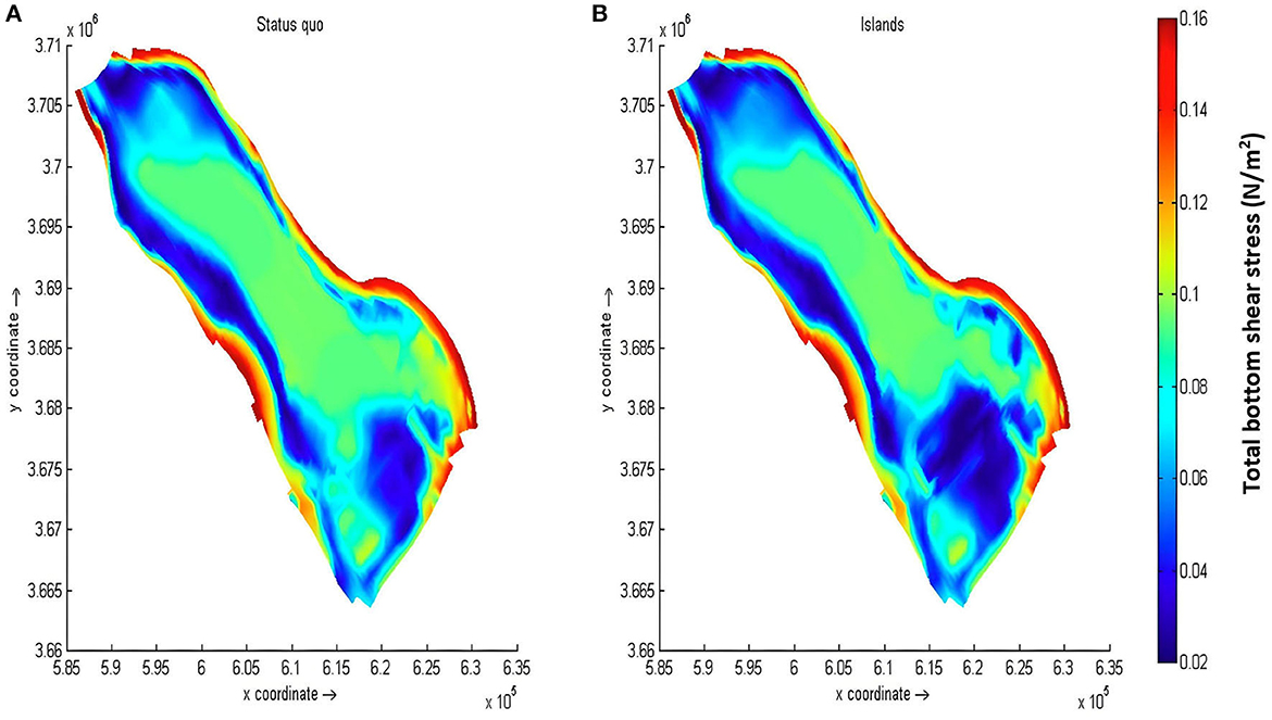
Figure 14. Comparison of the simulated maximum total bottom shear stresses in (A) the status quo condition and (B) in the presence of islands in September 2005.

The critical bottom shear stress is 0.0625 N/m² estimated using the representative sediment size of 25 μm in the Salton Sea (Chung et al., 2009a). Below this critical threshold, the constraint conditions used in the resuspension formulation in Delft3D-WAQ would carry out the shear stress limitation function as zero, resulting in no resuspension activity. The decrease of total bottom shear stress in the south basin confirmed the orthophosphate concentrations decline in the presence of islands. Moreover, the simulation indicated that the area covered by the islands was shielded from bottom shear stress exceeding the critical level (darker blue region), which in the long term, could enhance burial effects that lead to orthophosphate removal in the water column.

3.4.6. Salinity

The salinity in the status quo and the two mitigation strategies are compared in Figure 15. The nearly 2-year simulation showed a distinct discrepancy in salinities with and without the seawater import/export implementation. The starting salinity on September 1, 2005, was 46 ppt and decreased steadily to the range of 38 to 39 ppt by August 8, 2007. The change of the salinity was resolved well by the FLOW module and was consistent with the mass balance estimation, which indicated that the salinity would start to stabilize at 38 ppt in 2.47 years.

FIGURE 15

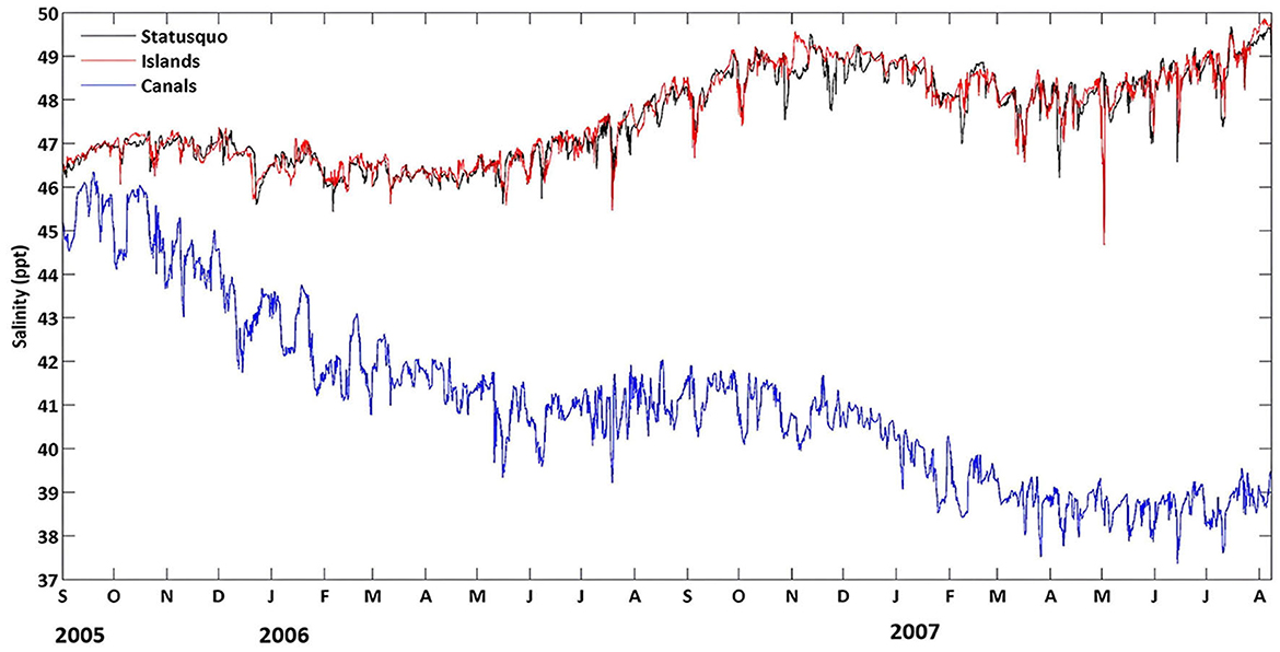
Figure 15. Comparison of the simulated salinity progressions in the status quo condition (black line), in the presence of emerged islands (red line), and the seawater importation scenario (blue line) from 9/1/2005 to 8/8/2007.

The fluctuation in the salinity progression corresponded to water level fluctuation, which was directly associated with seasonal variation of tributary river flow rates. Figure 15 also shows that salinity would not be affected by the presence of islands in the southern basin.

4. Discussion

4.1. Summary and conclusions

4.1.1. Delft3D-WAQ simulation results for the status quo Salton Sea

In this study, three Delf3D modules: Delft3D FLOW, Delft3D WAVE, and Delft3D-WAQ within the Delft3D modeling suite were utilized to investigate the water quality dynamics of the Salton Sea in the status quo and three mitigation scenarios from 9/1/2005 to 8/8/2007.

Using the hydrodynamic information derived from the FLOW and WAVE modules, the WAQ module generated suspended sediment concentration and total bottom shear stress that were in good agreement with the pattern and timing of the measured data. Later on, the WAQ module was calibrated and validated against the quarterly dataset collected by the Bureau of Reclamation for the water quality variables of interest, including dissolved oxygen, orthophosphate, unionized ammonia, and chlorophyll a.

The simulated DO concentration throughout the water column was in reasonable range as the measured data. However, the DO concentrations on the top surface layer were not accounted for due to vertical grid limitation, leading to a general underestimation on the surface level, except in July. Nonetheless, the DO concentration in the bottom layer was in good agreement with the measured values.

Seasonal fluctuations of unionized ammonia were resolved well and within a reasonable range by The WAQ module. Simulated results from the central south basin showed better agreement with the measured values than the central north basin. The input unionized ammonia concentrations in the inflows were set at constant values using the average of the quarterly data from September 2005 to May 2007; the uncertainties derived from the inflow nutrient concentrations contributed to the 24 to 66% difference to the observed values in the south-central and north-central basins, respectively.

The overestimation of orthophosphate concentrations originated from various uncertainties and assumptions in the computation processes (sorption, precipitation, autolysis, and mineralization) for orthophosphate simulation. Nonetheless, the results showed that the sediment resuspension flux corresponded well to wind velocity magnitudes, and that the fate and transport of orthophosphate concentrations in the water column is intricately linked to this wind-driven mechanism. Lastly, the simulation of algal productivity resolved the seasonal trend for chlorophyll a concentration that followed the measured trends rather well, except for under-estimation in mid-February 2007 (data not shown).

Overall, the WAQ module presented in this work successfully resolved two most significant phenomena that determine the water quality dynamics of the Salton Sea: thermal stratification and sediment resuspension activities. The results confirmed the findings of previous studies that wind-driven sediment-resuspension events are the main driving force to influence the Sea's nutrient cycling (Chung et al., 2008, 2009a).

4.1.2. The critical role of a water quality modeling framework in Salton Sea restoration

Having a three-dimensional dynamic water quality/hydrodynamic model that is tailored to the unique system of the Salton Sea is imperative in order to achieve the statutory restoration goals as required by the State Water Board Revised Oder WR 2002-0013 and the Salton Sea Restoration Act [Fish and Game Code § 2931, subdivision (c)]. However, in the past two decades, lead government agencies have been evaluating the overall feasibilities of various proposed long-range Salton Sea restoration concepts mainly based on water and salts balance models such as the Salton Sea Analysis Model (SALSA, SALSA2) and Salton Sea Accounting Model (SSAM) (Reclamation, 2007; Salton Sea Authority, 2016; CH2M, 2018; CNRA, 2022).

The Salton Sea Management Program (SSMP) drafted a Long-Range Plan as a second phase after Phase I: 10-year Plan, in which SSMP evaluated 13 restoration concepts that are evaluated based on their overall functions to not only combat the environmental challenges associated with the anticipated recession of the Sea beyond 2028 but also provide multiple environmental/recreational benefits.

In order to select the optimal long-term restoration plan for the Salton Sea, it is crucial that detailed evaluations are conducted based on accurate analyses using validated and robust models. At the current stage of the planning process, SSMP has identified four key areas of uncertainties associated with future inflows, public health impact due to air quality, ecological outcomes, and economic development. Nonetheless, among those areas of uncertainties, the water quality of the Salton Sea is the most influential factor and the root cause of the uncertainties, given the footprint of the water body. Yet, its impact is accounted for the least due to the lack of adequate water quality models.

Hydrologic models such as SALSA and SSAM can be used to simulate a wide range of configurations/conservation efforts (i.e., habitats, wetlands, and divided Sea, etc.) in an uncertainty framework; they were operated in the stochastic model to simulate conditions in the Sea for each of the possible input traces, providing a range of future outcomes of inflows, salt loads, elevations, precipitation, and evaporation rates. It is worth noting that in the most recent “Salton Sea Long-Range Plan,” published in December 2022, the same stochastic and deterministic Excel spreadsheet model, SSAM, was still the primary modeling approach used to assess proposed restoration alternatives since 2007. All restoration concepts were evaluated under three future hydrology scenarios (high, low, and very low probability inflows) on an annual timestep for only salinity and elevation forecasts (CNRA, 2022).

Without a validated water quality model to analyze the restoration concepts' potential influences on water quality of the Sea, habitat areas located within the Salton Sea footprint, and the inflowing waters, the SSMP has deemed ALL 13 proposed plans scored three out of five in their ability to improve water quality, majority of the concepts scored full score in their ability to meet selenium standards, suggesting that the features such as sedimentation basins, flow-through systems, and export of high nutrient Salton Sea water are adequate and sufficient to provide beneficial uses and reduce environmental consequence. In addition, SSMP recommended the divided Sea concept for further evaluation because it scored highest in all categories in both the high and low probability inflow scenarios (CNRA, 2022).

However, this recommendation contradicted the assessment conducted by the Bureau of Reclamation in 2007; the summary report stated that there are operational uncertainties associated with each major feature: marine lake, brine pool, the species conservation habitat, and sediment retention basins, as they altered the current combination of physical, chemical, and biological components in the Sea. The following situations could lead to an increase of Se concentration in the alternatives: (1) shallower residual Sea or reduced size marine lakes are more prone to wind mixing that facilitates strong resuspension of Se bearing sediments, (2) a more oxygenated system or a highly saline system may inhibit anaerobic bioremediation of Se from the water column, (3) alternate wetting and drying of exposed sediment would facilitate formation of ephemeral pools with high Se levels, (4) decreased drainage volume would increase Se concentration entering the Sea to as high as 8 to 18 μg/L (Reclamation, 2007).

Moreover, the report further stated that the divided Sea with the south marine lake offered the second highest risk among the five alternatives because of the potential high risk to the fishery from salinity/temperature variations, prolonged stratification, hypereutrophic conditions with occasional, severe oxygen depletion, and Se bioaccumulation risk to invertebrate eating breeding birds.

Previous studies have demonstrated that comprehensive hydrodynamics/water quality models customized for the Salton Sea have significant implications in assessing potential impacts of the water quality dynamics under various restoration strategies (Cook et al., 2002; Holdren and Montaño, 2002; Chung et al., 2008, 2009a). In the early 2000s, multiple research groups utilized a deterministic model and numerical models validated for the Salton Sea's system to simulate different proposed restoration plans' impacts on the Salton Sea's hydrodynamics and the consequential water quality dynamics of the water body.

A three-dimensional hydrodynamic numerical model, RMA10, was applied to evaluate circulation changes under the conditions created by four proposed diking alternatives. Cook et al. (2002) demonstrated that north/south ponds and displacement dike in the Delta areas of the two rivers led to disproportional increased and decreased local velocities around the diked impoundment areas and large stagnation zones (Cook et al., 2002). Chung et al. (2008, 2009a) made the first attempt combining sediment resuspension models with a one-dimensional hydrodynamic/water quality model (Dynamic lake model-water quality, DLM-WQ) to investigate the effect of sediment resuspension on nutrient cycling in the Salton Sea. DLM-WQ is a process-based, deterministic model based on a Lagrangian layer scheme. The calibrated model was used to simulate a scenario of 90% external tributary phosphorus load reduction. The results indicated minor short-term effects on chlorophyll a concentration and phytoplankton growth. Therefore, it was deduced that internal loading caused by sediment resuspension plays a vital role in contributing to the nutrient budget within the Sea. In addition, simulations suggested that nutrients concentration were higher in the South Sea scenario than in the full Sea due to stronger wind-driven sediment resuspension events in shallower water depths (Chung et al., 2008). Rueda et al. (2009) evaluated the effects of a reduced lake (the North Sea scenario) on thermal stratification using another three-dimensional numerical model (Si3D). The results indicated that reducing the lake size would induce a stronger and longer stratification, often associated with hypolimnetic oxygen depletion and major die-offs of aquatic life (Rueda et al., 2009).

4.1.3. Delft3D-WAQ applications on water quality mitigation strategies simulations of the Salton Sea

In this study, Delft3D-WAQ was utilized to assess the impacts on the Salton Sea's water quality under three water mitigation strategies, including a nature-based solution, a seawater import/export concept, and the water importation along with inflows water pollution control strategy. The design of the emerged islands as a nature-based solution to mitigate Salton Sea's water quality served two purposes, (1) to interfere with inflows that contained high nutrient concentrations and suspended sediments from transporting norward to the entire Sea, and (2) to reduce wind fetch, thereby reducing the bottom shear stress that affects wind-induced sediment resuspension activities. Reduced sediment resuspension had a limited effect on DO and NH₃, as the results showed less than a 40% increase in DO and approximately 6.3% decreased NH₃ during the summer season.

The fact that unionized ammonia merely decreased by 6.3% in the presence of emerged islands in the south basin suggested that unionized ammonia accumulation was not influenced by wind-fetch and wind-driven sediment resuspension activities. On the other hand, emerged islands effectively reduced bottom shear stress, and the PO₄ concentration decreased by 18 and 31% during the first and second storms, respectively, compared to the status quo. After the first simulation year, orthophosphate concentrations remained about 5% lower (< 0.06 mg/L) than in the status quo condition from September 2006 until August 2007. Furthermore, the simulation showed that high algal productivity was contained in the south basin, where chlorophyll a concentrations were at a lower range of 350–400 μg/L compared to 400–500 μg/L in the same region in the status quo condition from 4/1/2007 to 6/30/2007.

The effectiveness of importing and exporting seawater in reducing salinity and improving water quality was evaluated in this study. Having imported aerated, nutrients-free seawater at the discharge rate of 225 m³/s from the southwestern shore and exporting lake water at 215.5 m³/s in the northwestern shore, the DO concentration increased more than 50% throughout the water column from 7/1/2006 to 9/30/2006. The PO₄ concentrations in the north basin experienced a more significant decline than in the south basin (14 and 8.3%, respectively) during the first storm in September 2005. Orthophosphate concentration in the central north and south basin remained constant, decreasing percentages at approximately 5 to 8% as simulation time progressed.

Contrary to the slight decline of PO₄ concentration in the Sea, import/export canal implementation effectively removed unionized ammonia NH₃ and resulted in an approximately 49.3% decrease during the peak of summer 2006 and a steady decline as simulation time progressed. The maximum chlorophyll a concentration during Spring in 2007 in the canal scenarios was much lower than the status quo and the emerged island scenarios; chlorophyll a concentrations were in the range of 250–300 μg/L and appeared to be scattered in the Sea with only the central basin had higher Chl a concentration up to approximately 350 ug/L. Finally, the seawater import/export scenario showed that it would take 2 years for salinity to fluctuate but steadily decrease from 46 ppt to 38–39 ppt, consistent with the mass balance calculation that estimated salinity would start to stabilize at 38 ppt in 2.47 years.

In the most robust water quality mitigation scenario, where nutrients in the tributary rivers were reduced by 90% in addition to seawater canal implementation, the results showed a drastic decline of PO₄ concentrations merely 2 months into the simulation. Toward the end of the nearly 2 years simulation, the PO₄ concentrations were as low as 0.01 mg/L in the Salton Sea. In addition, unionized ammonia concentration decreased by 68.3% by August 2007. The chlorophyll a concentration and DO hugely depend on algal productivity, computed by optimization technique in the BLOOM module. The growth and mortality constraints prevent a single algae species from being removed within a single time step and maximize the total net growth. As a result, the WAQ module presented the same chlorophyll a and DO concentrations in two canal scenarios where nutrient concentrations declined too rapidly.

In summary, the simulation results showed that having emerged islands in the south basin of the Salton Sea can be an effective nature-based solution to improve the water quality in the long term because the natural burial processes in the sediments are weaved into the built environment to achieve low-impact resilience to wind-driven bottom shear stress without significantly disturbing natural lake stratification. In addition, the simulations of the water importation concept indicated that importing nutrients-free seawater and exporting the Salton Sea's water at roughly the same rates are more effective in decreasing NH₃ than PO₄ concentrations in the system. Finally, the Delft-WAQ model demonstrated that having treated inflow waters (90% nutrients reduction) in addition to the water importation/exportation implementation can overcome internal loading events and drastically decrease orthophosphate concentration in 2 months. Nonetheless, this robust strategy still could not reduce the unionized ammonia level in the Salton Sea to below the critical level of 0.05 mg/L in 2 years.

Overall, the Delft3D numerical water quality modeling framework is capable of simulations for non-steady flow and transport phenomena/water quality processes resulting from meteorological forcing in three dimensions, which provides a better understanding of thermal stratification and wind-driven sediment resuspension events in influencing nutrient cycling and phytoplankton growth that take place in the water column and sediment layers of the Salton Sea. The results presented in this work not only further confirmed the significance of internal loading on affecting the water quality of the Salton Sea but also indicated that the water importation/exportation restoration concept, while effective in reducing salinity by 17% in 2 years, has little impact on decreasing nutrients concentrations in the Salton Sea. Nonetheless, the simulations showed promising results in having emerged islands as a nature-based solution to mitigate water quality in the long term.

4.2. Future direction and recommendations

The calibration and validation tasks for the FLOW/WAVE modules in this study were based on two <2 months of field measurements taken in 1999 and 2005, respectively, from two previous studies conducted by Huston et al. (2000) and Chung et al. (2009b). To be consistent with the validated hydrodynamics conditions, the WAQ module was calibrated/validated using the dataset collected quarterly by the Bureau of Reclamation in 2005. The most vital step to building a model tailored to current hydrodynamic conditions is to initiate another monitoring campaign in the future to measure relevant parameters such as wave height, wave period, current velocity, etc. In addition, it has been established that sediment adsorption is critical to orthophosphate internal loading in the water column. Therefore, a more intensive, long-term monitoring program (monthly or bi-weekly) at the tributary rivers' mouths and every 1–2m depth for the north, center, and south basins in the Sea to collect sediment/water quality samples for sediment concentration/composition, thereby orthophosphate adsorption capacity analysis would help estimate orthophosphate concentration in the sediment and water column of the Sea more precisely.

The biogeochemical cycles in the Salton Sea are heavily influenced by sediment composition and sediment diagenesis. In this work, the sediment-water interaction is modeled by the simplified S1/S2 approach, where the sediment layers are subject to settling, resuspension, burial, and digging processes for the settled substances that are mineralized. Since the sediment layers share the same computational grid as the overlying water, mineralization in the sediment layers would lead to instantaneous oxygen consumption in the entire water column, which influenced the accuracy of the overall water quality simulation. Future work should consider using D-Water Quality software with extended functionalities that allow users to create a separate computational grid for the active sediment layer, having been able to compute redox reactions of sulfate, dissolved sulfide, particulate sulfide, apatite-phosphate, vivianite-phosphate, methane that take place in the deep sediment boundary layer allows a more comprehensive simulation of the fate and transport of nutrients and sulfate in the Salton Sea.

The 2-year simulation timeframe carried out in this study is the longest water quality simulation of the Salton Sea performed so far. However, while the FLOW module is capable of resolving water level decline due to the high evaporation rate in the Salton Sea, the rapid water loss would lead to an overestimation of critical water quality variables in the WAQ module. The issue could be solved by excluding the non-local sink term of evaporation in the continuity equation. Nonetheless, this highlights the limitation of the WAQ module on handling fast decline water levels in aquatic systems in an arid region like the Salton Sea. Moreover, the maximum threshold for salinity calculation in the FLOW module is 50 ppt. As a result, to simulate the current Salton Sea (74.25 ppt as of January 2020, measured by BOR), an equation of state for hypersaline water needs to be integrated into existing Delft3D-FLOW to accurately characterize the spatial-temporal changes in density structure that affect temperature and salinity simulation directly.

Without a validated, three-dimensional hydrodynamics/water quality model, biased or overly optimistic assessments based on false assumptions may lead to ineffective or incorrect evaluations of the overall Salton Sea restoration concepts. To predict future Salton Sea elevation, volume, surface area, and salinity based on inflow projections using merely a one-dimensional salt and water balance accounting model only allows planning developments occurring on the exposed playa where there's no water. Relying heavily on SSAM for the Salton Sea's resource management tasks has been limiting the Salton Sea Management Program to addressing challenges of the Salton Sea from only the land perspective.

However, what will happen within the largest footprint of every alternative configuration plan -the water body of the Salton Sea- remains yet to be discovered. In other words, the state of water quality of the Salton Sea, which hugely determines the ecological and recreational values of the Sea, should take the central stage of any restoration efforts in the future. Failing to address the biggest puzzle of the Sea itself but simultaneously planning for potential recreational/ecological usage and economic development directly from and around the Salton Sea is counterintuitive; the chance of once again failing to deliver the statutory restoration goals for the Salton Sea is very high. Instead of identifying water quality as a low-priority factor of relevant uncertainties, a robust and comprehensive, three-dimensional water quality/hydrodynamic model such as presented in this work allows more cost-effective and innovative restoration concepts to be effectively assessed and should be operated alongside SSAM for future planning for the Salton Sea.

Data availability statement

Publicly available datasets were analyzed in this study. This data can be found here: https://www.usbr.gov/lc/region/programs/saltonsea.html, https://cimis.water.ca.gov/WSNReportCriteria.aspx, https://waterdata.usgs.gov/monitoring-location/10254005/#parameterCode=62614&period=P7D.

Author contributions

M-CL contributed to conceptualization, design, data analysis, execution of the study, and wrote the original manuscript. All authors contributed to manuscript revision, read, and approved the submitted version.

Acknowledgments

The authors would like to acknowledge Deltares for the technical supports, Bureau of Reclamation- Lower Colorado Region, United States Geological Survey, The California Irrigation Management Information System, and NASA Jet Propulsion Laboratory for providing bathymetry, water quality and meteorological datasets of the Salton Sea. Special appreciation goes to Christopher B. Cook, Dr. E. G. Chung, F. A. Bombardelli, F. Rueda, J. Vidal, and S. G. Schladow for the valuable research on Salton Sea hydrodynamics and water quality simulations that have become the foundation of my study.

Conflict of interest

The authors declare that the research was conducted in the absence of any commercial or financial relationships that could be construed as a potential conflict of interest.

Publisher's note

All claims expressed in this article are solely those of the authors and do not necessarily represent those of their affiliated organizations, or those of the publisher, the editors and the reviewers. Any product that may be evaluated in this article, or claim that may be made by its manufacturer, is not guaranteed or endorsed by the publisher.

References

Amorocho, J., and DeVries, J. J. (1980). A new evaluation of the wind stress coefficient over water surfaces. J. Geophys. Res. 85, 433–442. doi: 10.1029/JC085iC01p00433

CrossRef Full Text | Google Scholar

Barnum, D. A., Bradley, T., Cohen, M., Wilcox, B., and Yanega, G. (2017). State of the Salton Sea—A science and monitoring meeting of scientists for the Salton Sea (No. 2017-1005). US Geological Survey. doi: 10.3133/ofr20171005

CrossRef Full Text | Google Scholar

California Department of Public Health (n.d.). California Breathing. Available online at: https://www.cdph.ca.gov/Programs/CCDPHP/DEODC/EHIB/CPE/Pages/CaliforniaBreathingCountyAsthmaProfiles.aspx (accessed May 8 2019).

Google Scholar

CH2M (2018). Salton Sea Hydrology Development. Available online at: https://www.iid.com/home/showpublisheddocument/17297/636763993646630000

Google Scholar

Chung, E. G., Bombardelli, A., and Schladow, S. G. (2009a). Sediment resuspension in a shallow lake. Water Resour. Res. 45, 1–18. doi: 10.1029/2007WR006585

CrossRef Full Text | Google Scholar

Chung, E. G., Bombardelli, F. A., and Schladow, S. G. (2009b). Modeling linkages between sediment resuspension and water quality in a shallow, eutrophic, wind-exposed lake. Ecol. Model. 220, 1251–1265. doi: 10.1016/j.ecolmodel.2009.01.038

CrossRef Full Text | Google Scholar

Chung, E. G., Schladow, S. G., Perez-Losada, J., and Robertson, D. M. (2008). “A linked hydrodynamic and water quality model for the Salton Sea,” in The Salton Sea Centennial Symposium: Proceedings of a Symposium Celebrating a Century of Symbiosis Among Agriculture, Wildlife and People, 1905–2005, held in San Diego, California, USA, March 2005 (Netherlands: Springer), 57–75. doi: 10.1007/978-1-4020-8806-3_5

CrossRef Full Text | Google Scholar

CNRA (2022). Salton Sea Management Program: Long-Range Plan, Public Draft. Available online at: https://saltonsea.ca.gov/wp-content/uploads/2022/12/Salton-Sea-Long-Range-Plan-Public-Draft-Dec-2022.pdf

Google Scholar

Cohen, M. J., Morrison, J. I., and Glenn, E. P. (1999). Haven or Hazard : The Ecology and Future of the Salton Sea. Oakland, CA: Pacific Institute for Studies in Development, Environment and Security.

Google Scholar

Cohn, J. P. (2000). Saving the Salton Sea. BioScience 50, 295–301. doi: 10.1641/0006-3568(2000)050(0295:STSS)2.3.CO;2

CrossRef Full Text | Google Scholar

Cook, C. B., Orlob, G. T., and Huston, D. W. (2002). Simulation of wind-driven circulation in the Salton Sea: Implications for indigenous ecosystems. Hydrobiologia 473, 59–75. doi: 10.1023/A:1016517331869

CrossRef Full Text | Google Scholar

Deltares (2014). D-Water Qaulity: Process library description-Technical reference manual. Delft. Available online at: https://content.oss.deltares.nl/delft3d4/D-Water_Quality_Processes_Technical_Reference_Manual.pdf

Google Scholar

Deltares (2020). Delft3D-FLOW User Manual: Simulation of multi-dimensional hydrodynamic flows and transport phenomena, including sediments. Deltares. Available online at: https://content.oss.deltares.nl/delft3d4/Delft3D-FLOW_User_Manual.pdf

Google Scholar

Farzan, S. F., Razafy, M., Eckel, S. P., Olmedo, L., Bejarano, E., and Johnston, J. E. (2019). Assessment of respiratory health symptoms and asthma in children near a drying saline lake. Int. J. Environ. Res. Public Health 16, 3828. doi: 10.3390/ijerph16203828

PubMed Abstract | CrossRef Full Text | Google Scholar

Ferreira, M., and Stenstrom, M. K. (2013). The importance of particle characterization in stormwater runoff. Water Environ. Res. 85, 833–842. doi: 10.2175/106143013X13736496909103

PubMed Abstract | CrossRef Full Text | Google Scholar

Hely, A. G., Hughes, G. H., and Irelan, B. (1966). Hydrologic Regimen of Salton Sea, California. Washington, DC: US Government Printing Office. doi: 10.3133/pp486C

CrossRef Full Text | Google Scholar

Holdren, G. C., and Montaño, A. (2002). Chemical and physical characteristics of the Salton Sea, California. Hydrobiologia 473, 1–21. doi: 10.1023/A:1016582128235

CrossRef Full Text | Google Scholar

Hughes, B. (2020). Turning off the tap: will California let the Salton Sea go down the drain? California Western Law Rev. 56, 8. Available online at: https://scholarlycommons.law.cwsl.edu/cwlr/vol56/iss1/8

Google Scholar

Huston, D. W., Cook, C. B., and Orlob, G. T. (2000). “New and alamo rivers project - preliminary data collection and analysis of development of hydrodynamic and water quality river models,” in Water Resources and Environmental Modeling Group, Department of Civil and Environmental Engineering [and] Center for Environmental and Water Resources Engineering, University of California, Davis.

Google Scholar

Knowlton, M. F., and Jones, J. R. (1995). Temporal and spatial dynamics of suspended sediment, nutrients, and algal biomass in Mark Twain Lake, Missouri. Arch. Hydrobiol. 135, 145–178. doi: 10.1127/archiv-hydrobiol/135/1995/145

CrossRef Full Text | Google Scholar

Krone, R. (1962). Flume studies of transport of sediment in estuarial shoaling processes. Technical report.

Google Scholar

Lee, M. (2021). Water Quality Mitigation Strategy Analysis of the Salton Sea, California Using the Delft-3D Modeling Suite. UCLA. Available online at: https://escholarship.org/uc/item/1sx8g06v (accessed October 22, 2021).

Google Scholar

Li, Y., Lau, S. L., Kayhanian, M., and Stenstrom, M. K. (2006). Dynamic characteristics of particle size distribution in highway runoff: Implications for settling tank design. J. Environ. Eng. 132, 852–861. doi: 10.1061/(ASCE)0733-9372(2006)132:8(852)

CrossRef Full Text | Google Scholar

Little Hoover Commission (2015). Averting Disaster: Action now for the Salton Sea. A Little Hoover Commission Letter Report to the Governor and Legislature of California.

Google Scholar

Marti-Cardona, B., Steissberg, T. E., Schladow, S. G., and Hook, S. J. (2008). “Relating fish kills to upwellings and wind patterns in the Salton Sea,” in The Salton Sea Centennial Symposium: Proceedings of a Symposium Celebrating a Century of Symbiosis Among Agriculture, Wildlife and People, 1905–2005, held in San Diego, California, USA, March 2005 (Netherlands: Springer) 85–95. doi: 10.1007/978-1-4020-8806-3_7

CrossRef Full Text | Google Scholar

Partheniades, E. (1962). A Study of Erosion and Deposition of Cohesive Soils in Salt Water. University of California, Berkeley, USA.

Google Scholar

Reclamation, B. (2007). Restoration of the Salton Sea Summary Report. Boulder City.

Google Scholar

Rueda, F., Vidal, J., and Schladow, G. (2009). Modeling the effect of size reduction on the stratification of a large wind-driven lake using an uncertainty-based approach. Water Resour. Res. 45, 988. doi: 10.1029/2008WR006988

CrossRef Full Text | Google Scholar

RWQCB (1998). New River pollution in Mexico, a historical overview. Regional Water Quality Control Board.

Google Scholar

Salton Sea Authority (2016). Salton Sea Funding and Feasibility Action Plan Benchmark 7: Project Summary. Available online at: http://saltonseaauthority.org/wp-content/uploads/2017/02/SS-Benchmark-7_5-11-16r.pdf (accessed March 7, 2018).

Google Scholar

Setmire, J. G., Wolfe, J. C., and Stroud, R. K. (1990). Reconnaissance investigation of water quality, bottom sediment, and biota associated with irrigation drainage in the Salton Sea area, California, 1986-87. U.S. Geological Survey, U.S. Fish and Wildlife Service, U.S. Bureau of Reclamation.

Google Scholar

Taylor, P. A., and Lee, R. J. (1984). Simple guidelines for estimating wind speed variations due to small-scale topographic features. Climatol. Bull. 18, 3–32.

Google Scholar

U.S. EPA (2005). Development of water qaulity analyses for the shared waters of the US and Mexico. United States Environmental Protection Agency Office of Wastewater Management, RTI International.

Google Scholar

Watts, J. M., Swan, B. K., Tiffany, M. A., and Hurlbert, S. H. (2001). “Thermal, mixing, and oxygen regimes of the Salton Sea, California, 1997–1999,” in Saline Lakes: Publications from the 7th International Conference on Salt Lakes, held in Death Valley National Park, California, USA, September 1999 (Netherlands: Springer), 159–176. doi: 10.1007/978-94-017-2934-5_15

CrossRef Full Text | Google Scholar