Study of height-spread sporadic-E layers observed in the South American Magnetic Anomaly

Spread echoes from the E-region observed in ionograms obtained at high latitudes are generally classified as auroral sporadic-E (Esa) layers. These layers have also been detected in nighttime ionograms collected at some ionospheric stations in the South American Magnetic Anomaly (SAMA) region in Brazil during the recovery phases of geomagnetic storms. However, similar echoes have also been observed in the SAMA during geomagnetically quiet periods or daytime, which are not caused by energetic particle precipitation. Therefore, investigating the occurrence of these spread echoes over a longer period, rather than focusing solely on case studies, has become important. Thus, this study aims to analyze the occurrences of spread echoes from the E-region, referred to here for the first time as “Height-Spread Es (HSEs) layers.” The analysis is based on Digisonde data obtained at the Santa Maria station (29.7° S, 53.8° W, ∼22.000 nT) in Brazil over 1 year (2019/2020). The study initially presents examples of these traces on ionograms and then examines their occurrence rates over several time intervals (hours, months, seasons). Among other findings, the statistical analysis reveals that the occurrence rate of HSEs layers is 9.8% during the analyzed period. The HSEs layers appeared predominantly at night and under geomagnetically quiet conditions. Most HSEs layers lasted between 1 h and 3 h 30 min, with a peak incidence during November, December, and January. Finally, the study discusses the most likely mechanisms responsible for HSEs layer formation, considering the geomagnetic conditions and time of their detection on ionograms.

1 Introduction

The Sporadic-E (Es) layers produce unmistakable traces in ionograms with characteristics that depend on the station where they are detected. In the low and middle latitude stations, the Es layers are produced by the redistribution of meteor ionization caused by the wind shear mechanism (Mathews, 1998; Whitehead, 1961). This mechanism moves clouds of metallic and molecular ions to a thin layer at heights of the mesosphere and lower thermosphere (∼100–150 km) region. When sufficiently dense, Es layers can significantly affect the radio wave propagation by reflecting high-frequency (HF) and very-high-frequency (VHF) signals, effectively acting as a mirror (McNamara, 1991). The strong vertical electron density gradients associated with Es layers can cause severe ionospheric scintillations in the Global Navigation Satellite System (GNSS) signals, sometimes leading to complete signal loss (Vankadara et al., 2022; Yu et al., 2020; Seif et al., 2017; Yue et al., 2016; Zeng and Sokolovskiy, 2010). Es layers also impact the HF signals used in the over-the-horizon radars, which are important for aviation and military applications (Cameron et al., 2022). Additionally, Thayaparan and MacDougall (2005) examined the impacts of Es layers interference on high-frequency surface-wave radar for monitoring surface vessels and low-altitude air targets. For digital ionosondes, Es layers block the transmitted signal, preventing reflections from the F-region. These Es layers are named “blanketing” or Esb. Recently, Moro et al. (2022a), Moro et al. (2023) studied the Esb layers at Santa Maria (29.7° S, 53.8° W), Brazil, considering 1 year of Digisonde data (2019–2020). This ionospheric station is in an area with a remarkably low geomagnetic field intensity (∼22.000 nT) observed on the Earth. These works show that the SAMA influenced the Esb development over Santa Maria. In the data set obtained by the Digisonde from July 2019 to June 2020, the authors also found the presence of very scattered echoes from the E-region altitudes with a thickness of around 50 km. These echoes are classified here as Height-Spread Es (HSEs) layers. Their presence in the data motivated the development of the present study, since the echoes are completely different from the Esb layers. Indeed, the HSEs seem like those observed in the auroral regions known as auroral Es layer type (Esa). These layers, in turn, are caused by energetic particle streams from the outer radiation belt that precipitate in the Earth’s atmosphere and cause the excitation of oxygen and nitrogen. The Esa layers are short-lived and are characterized by a height-spread and diffuse pattern between 100–150 km in the ionograms (Resende et al., 2022a; Resende et al., 2022b; Zhang et al., 2015). Their formation mechanism is the wave (whistler-mode chorus, plume, magnetosonic waves)-particle resonances (Da Silva et al., 2023).

In a nonpolar region, as in the SAMA, Es layers that resemble the Esa usually appear in the ionograms collected during nighttime in the recovery phase of geomagnetic storms (Batista and Abdu, 1977; Da Silva et al., 2023; Moro et al., 2022b; Resende et al., 2023). For instance, Moro et al. (2022b) studied the Es layers development in the American sector during the August 2018 geomagnetic storm. The authors used Digisonde and the Radiation Belt Storm Probes (RBSP) Satellite (Mauk et al., 2013) to discover the formation mechanism. Among the results, the authors found the occurrence of Esa during the recovery phase over Santa Maria and Cachoeira Paulista (22.7° S, 45.0° W), both Brazilian stations inside the SAMA, due to wave (plasmaspheric hiss waves)-particle interactions. Da Silva et al. (2022) showed through RBSP data that the pitch angle scattering driven by hiss waves is indeed the mechanism responsible for low-energy electron precipitation in the SAMA during a geomagnetic storm caused by Interplanetary Coronal Mass Ejection–ICME. Da Silva et al. (2023) reported that the same mechanism also operated during a geomagnetic storm caused by High-Speed Solar Wind Stream (HSS). Resende et al. (2022b) studied the development of Es layers in several stations from auroral to low latitude regions during a HSS event. They observed signatures of Esa over Santa Maria during the recovery phase of the geomagnetic storm caused by plasmaspheric hiss waves, in agreement with Moro et al. (2022b) and Da Silva et al. (2022). The authors also observed Esa signatures over Tromso (69.7° N, 18° E), which was expected since the region is located in high latitude. There, the Esa were caused by the chorus waves, highlighting the different mechanisms acting in the low/middle and at high latitudes that causes the Esa, in agreement with Da Silva et al. (2023). Although inconclusive, the plasma wave-particle interaction mechanism was suggested to explain the particle precipitation in the SAMA during geomagnetic storms since the 1970’s (Batista and Abdu, 1977; Gonzalez et al., 1987; Jayanthi et al., 1997; Pinto and Gonzalez, 1986; Tsurutani et al., 1975), since the measuring techniques were not as sophisticated as compared to the RBSP era.

Despite several works showing cases of Esa development in the SAMA during geomagnetically disturbed periods, Resende et al. (2023) observed similar echoes over Cachoeira Paulista during geomagnetically quiet periods. These intriguing results indicated that other mechanisms need to be considered to explain the HSEs layers in the SAMA region. The authors attributed the formation mechanism to the Kelvin-Helmholtz Instability (KHI) since the particle precipitation mechanism was discarded through the analysis of RBSP data. The development of the KHI would affect the wind shear process causing the HSEs layers through gravity waves or unstable winds (Bernhardt, 2002; Resende et al., 2023). Another possibility raised by the authors would be the Gradient Drift Instability (GDI) development (Seif and Panda, 2024; Moro et al., 2016; Denardini et al., 2005). However, this instability is more effective in the equatorial region where the Equatorial Electrojet occurs.

Considering the possibilities of charged particle streams precipitation, plasma instabilities as KHI, GDI, or other phenomena still unknown in producing the HSEs layers in ionograms collected inside the SAMA, studies about their occurrences in a more extended period, not only during case studies, is very important. Therefore, the purpose of this work is to present a comprehensive investigation of HSEs layers observed in Digisonde data collected in Santa Maria from July 2019 to June 2020, a station located close to the SAMA center, where the geomagnetic field intensity is ∼22.000 nT. Initially, the work focuses on the presentation of the HSEs layers on ionograms during all conditions: geomagnetically disturbed and quiet, nighttime, and daytime. After that, the occurrence rates of HSEs layers are discussed in several units of time (hours, months, seasons). Finally, the most likely mechanisms responsible for the HSEs layer formation are also presented and discussed.

2 Instrumentation and methods

The data recorded from a Digisonde Portable Souder – 4D (DPS-4D) installed at Santa Maria station (URSI code SMK29) is used to study the HSEs layer occurrences from July 2019 to June 2020. This period comprehends low solar activity with few geomagnetic storms classified as weak or moderate. The DPS-4D transmits radio waves from 0.5 to 30 MHz with a step of 25 kHz every 5 min. This means 288 ionograms can be obtained after 24 h of sounding (Moro et al., 2019).

To study the seasonal behavior of the HSEs layers in this station located in the Southern Hemisphere, the data collected in June, July, and August are representative of austral winter, and September, October, and November are representative of spring. The data measured between December and February corresponds to summer, and autumn is given by data obtained from March to May. During the studied period, the solar activity was low, with the solar 10.7 cm radio flux (F10.7) around 65 (in solar radio flux unit equal to 10⁻²²Wm⁻² Hz⁻¹). The data are classified according to the Kp index. The data are considered geomagnetic disturbed when at least one of the eight Kp values in each day is higher than 3 (Kp > 3). Otherwise, the Digisonde data is classified as being geomagnetically quiet (Kp ≤ 3).

The DPS-4D data is analyzed with the software SAO-Explorer, which can identify the occurrences of Es layers through the visual inspection of all ionograms (∼83,000). During the inspection, the Es layers were classified into Esb (Esf, Esl, Esh, Esc) or HSEs layers. The Es layers were found in ∼46,000 ionograms. The occurrence rate (OR) is calculated according to Equation 1:

$OR=\frac{n}{M}\times 100\%(1)$

In this equation, n is the number of ionograms with observed HSEs layers during the period of study and M is the number of available ionograms in the same period. The OR is not affected if multiple traces of Es are observed simultaneously.

Table 1 shows the monthly distribution of the geomagnetically quiet and disturbed days from July 2019 to June 2020. Despite some data gaps due to technical maintenance in the equipment, 338 days were used to draw the statistics, 283 measured during geomagnetically quiet days, and 55 during geomagnetically disturbed days.

Table 1

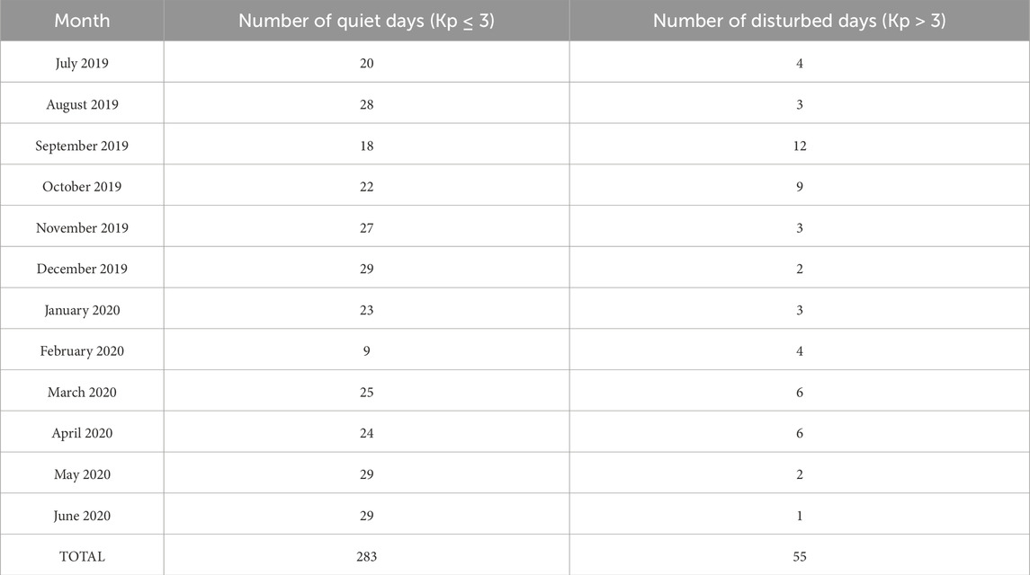
Table 1. Number of geomagnetically quiet and disturbed days (based on the Kp index) per month in which the Santa Maria Digisonde measured the HSEs layers.

Satellite data are used in this work. The Advanced Composition Explorer (ACE) satellite provides the interplanetary parameters during the moderate geomagnetic storm of September 2019. The RBSP satellite data are also considered to obtain information about the plasma waves present in the radiation belts during the presence of the Es layers in the ionograms. More specifically, the magnetic field power spectra density from the EMFISIS instrument onboard the RBSP satellite allows the identification of hiss waves in the plasmasphere, when the satellite is at the perigee. Since the RBSP data is available up to 13 October 2019, most of the case studies comprehend July, August, and September 2019. These selected cases are those when the RBSP is in the perigee orbit in low L-shells over the wide region of SAMA, when the HSEs layers were observed in the ionograms. Unfortunately, cases of HSEs layers during daytime occurred after 13 October 2019. Anyway, these cases are also presented in this work to show their characteristics.

3 Results and discussions

3.1 Presentation of height-spread Es layers

Some representative ionograms illustrating the spread traces from the E-region, HSEs layers, are shown in Figure 1. The ionograms present virtual reflection height (=1/2 cτ(f), where “c” is the free-space speed of light and “τ(f)” is the time in which the high frequency (f) signals travel) from 0 to 500 km in the ordinate, and the sounding frequency from 0 to 12 MHz in the abscissa. Each ionogram shows the date and hour in Universal Time (UT) when they were obtained. The Local Time (LT) is UT-3h. Moreover, the maximum Kp index observed in the day is indicated as a reference for the geomagnetic condition. The red arrows indicate the presence of height-spread echoes from the E-region, i.e., the HSEs layers. The HSEs echoes start at around 100 km and present a thickness of around 30–50 km or more in some cases. They occur with the Esf (nighttime)/Esl (daytime) Es in the background, typical Esb layers caused by the wind-shear mechanism that blanket the F-region. This behavior indicates that the HSEs layers may need the Esb layers in the background to occur. The physical mechanism responsible for echo scattering appears to intensify the layers rather than form them. At high latitudes, spread echoes from the E-region are generally referred to as Esa, as described by the Handbook of Ionogram Reduction and Interpretation (Piggott and Rawer, 1978). However, these echoes are classified in this work as HSEs layers because other mechanisms, such as irregularities, can be a potential ingredient for their formation.

Figure 1

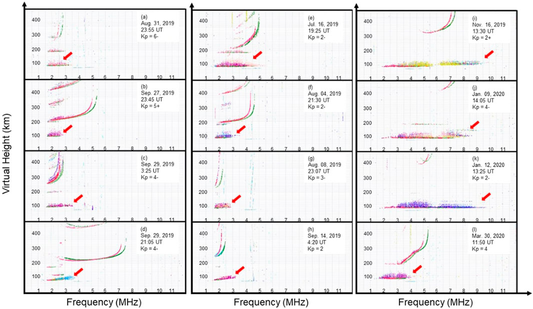
Figure 1. Ionograms recorded at Santa Maria (29.7° S, 53.8° W), Brazil, with red arrows showing the Height-Spread Es (HSEs) layers. Note that the ionograms are in UT (= LT + 3 h) and they were collected during (A–D) – geomagnetically disturbed conditions; (E–H) – geomagnetically quiet conditions; and (I–L) – daytime in geomagnetically quiet and disturbed conditions.

A comparative examination among the ionograms from Figure 1 reveals that the HSEs layers occur during several circumstances: geomagnetically disturbed conditions as in Figures 1A–D and geomagnetically quiet conditions in Figures 1E–H. In these examples, the HSEs layers occurred during nighttime. Nevertheless, they are also observed during daytime, as shown in Figures 1I–L, with different Kp values. The HSEs layers also present several characteristics regarding the top frequency (ftEs): low (<3 MHz) and high (>6 MHz). The thickness is around 50 km, sometimes achieving almost 80 km. They also present different direction-of-arrival, as shown by distinct pixel colors in the traces (the software uses “warm” colors for South direction and the “cold” colors for North). In general, low (high) ftEs values are observed during geomagnetically disturbed (quiet) conditions. During daytime, few cases presented high ftEs values compared to nighttime.

The temporal evolution of these HSEs traces is also irregular, as observed in the Esb layers. In other words, the HSEs layers can present sudden increases in their ftEs independently of the geomagnetic conditions and LT. The HSEs layers are also highly variable, however, differently from the typical Esb layers that are caused by the diurnal and semi-diurnal tides, the HSEs layers may be formed by different physical mechanisms as charged particle streams that precipitate due to the SAMA presence, very intense winds, or other phenomena unknown yet. In the next section, some statistics of the occurrence of these echoes are presented and discussed.

3.2 Occurrence rates (OR)

The visual inspection of ∼83,000 ionograms collected from July 2019 to June 2020 revealed the occurrences of HSEs layers in ∼8,100 ionograms, totalizing an OR (calculated with Equation 1) of 9.8% over Santa Maria (with no distinction between geomagnetically quiet and disturbed conditions). The HSEs layers also vary from month to month, as observed in the charts of Figure 2, in LT. The approximate time when the E-region over Santa Maria is illuminated by the Sun is highlighted in blue in the charts, and the period varies with months. The hourly OR values are placed on the vertical axis, and the LT hours are arranged radially in the clockwise direction, maintaining the same scale from 0% to 40% in all months except November and December, when the vertical axis ranges from 0%–50% and 0%–70%, respectively, due to the increase of HSEs layer occurrences.

Figure 2

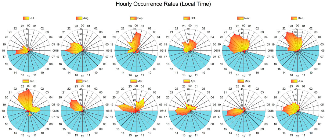
Figure 2. Hourly occurrence rates of spread echoes from the E-region in month of years 2019 (upper plots) and 2020 (bottom plots).

It is noteworthy that the HSEs echo occurrences are asymmetric at LT, with much more occurrences increasing soon before sunset to a peak of occurrence (that is different from month to month) and almost disappearing in the pre-sunrise period. Although most of them occurred during the nighttime, events of HSEs layers were also recorded during daytime. Figure 2 shows that the maximum OR is observed in December with a peak of ∼70% at 22 LT, and close to 60% at 21 and 23 LT. November and January also show high OR achieving ∼44% at 22 LT and 40% at 00 LT, respectively. The lower occurrences are in June, July, and August, which are the winter months. Indeed, studies report that Esb layers are very irregular and weak during winter over Santa Maria (Moro et al., 2023; Moro et al., 2022a). A clear seasonal dependence is observed, as complemented by Figure 3. It follows the same pattern as Figure 2 but notice that the vertical axis ranges from 0%–50% in Summer and 0%–30% in other seasons.

Figure 3

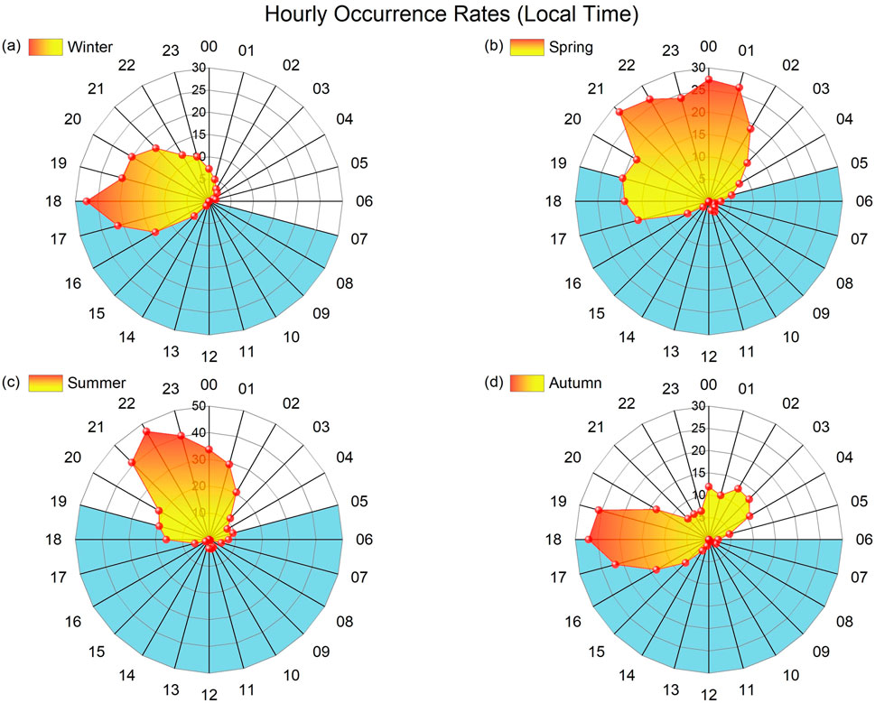
Figure 3. Hourly occurrence rates of spread echoes from the E-region for each season of the year: (A) Winter, (B) Spring, (C) Summer, and (D) Autumn.

The hourly OR of HSEs layers during the four seasons is presented in Figure 3. During winter (Figure 3A), the HSEs layers occurred more around sunset. The OR is lower than 5% from 01:00 to 15:00 LT. During spring (Figure 3B), the OR varies between 25% and 30% from 21 LT to 01 LT, while during other hours it presents values lower than 20%. In summer (Figure 3C), the OR achieves almost 50% of ionograms at 22 LT and ∼40% at 21 and 23 LT. The OR is very low during the daytime. The most irregular distribution is observed during the autumn (Figure 3D), when it seems that two periods are favorable to the occurrences of the HSEs layers, from 16 to 20 LT (around sunset at ∼18 LT) and between 2 and 4 LT, with OR varying between 10% and 15%.

Figure 4 presents the monthly and seasonal OR of HSEs layers. Figure 4A shows that November, December, and January present an OR between 15% and 20%. On the other hand, the other months presented OR lower than ∼10%. Figure 4B shows that the HSEs layers achieve more than 13% in summer and approximately 7% of occurrences in winter. Considering the equinoxes periods, spring presents a higher percentage occurrence of these spread echoes than autumn.

Figure 4

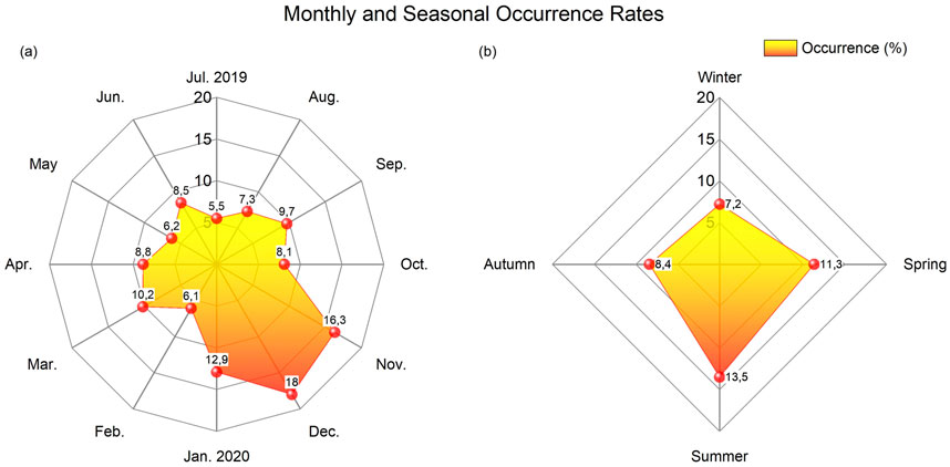
Figure 4. (A) Monthly and (B) seasonal occurrence rates of spread echoes from the E-region.

A significant finding of this study is, therefore, the variability in the HSEs occurrences across different months, seasons, and LT. Overall, the highest OR of HSEs layers is observed in summer, followed by spring, and during nighttime. The explanation of this behavior may be related to the close relation between the HSEs layers development with the Esb layers in the background. Therefore, since the Esb occurrences are maximum in summer due to the maximum meteor influx around this season of the year (Haldoupis, 2011), the HSEs layers may follow the same behavior. On the other hand, the Esb layers are weaker during winter because the amplitude of tidal winds is lower in this season. Moreover, during daytime, the HSEs layers are less frequent due to the high ionization of the ionosphere compared to nighttime, unless an intense mechanism (to be discussed ahead) is operating.

The duration of each HSEs event, which corresponds to the length of time they exist in the ionograms until disappears, varies from minutes to hours as shown in Figure 5. The first bar represents the HSEs with a duration up to 30 min. Only 1.6% of the events present this duration. The second bar is those HSEs that last from 30 min to 1 h. The occurrence increases to 6.2%. In the next case, which are events that last from 1h to 1 h 30 min, the occurrence achieves the highest value equal to 18.8%. Events of HSEs with duration between 2 and 3 h 30 min are less frequent but significant. A small number of events (less than ∼3%) presented duration a higher than 4 h. From July 2019 to June 2020, 308 events of HSEs were observed over Santa Maria.

Figure 5

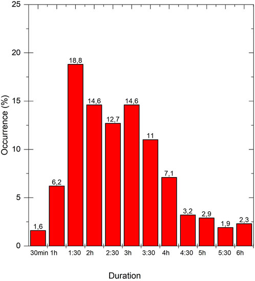
Figure 5. Histogram showing the percentage of occurrences of the HSEs layers from periods of 30 min intervals: 1.6% of events presented duration up to 30 min, 6.2% between 30 min and 1 h, 18.8% between 1 h and 1 h 30 min, and so on.

3.3 HSEs layers during geomagnetically disturbed conditions

After showing the OR of HSEs layers in several units of time (hours, months, seasons), this section presents and discusses some cases that occurred during geomagnetically disturbed conditions. Despite the data analysed in this work comprehends basically a period of low solar activity, few geomagnetically disturbed days with weak and moderate geomagnetic storms were observed from July 2019 to June 2020.

The ionogram in Figure 1A shows spread echoes in purple (from the west direction) between around 100 and 140 km height with ftEs ≅ 3 MHz. The ionogram was selected from an event of HSEs layers that lasted 1 h 15 min, from 22:40 to 23:55 UT on 31 August 2019. This period comprehends the main phase of a geomagnetic storm that started at 12:00 UT on the same day, when the north-south Bz component of Interplanetary Magnetic Field (IMF), not shown here, remained below zero due to the influence of an HSS. The source of the higher solar wind field was an event of corotating interaction region combined with solar sector boundary crossing event. Since the RBSP orbit was far from SAMA region during the period of HSEs layer occurrences over Santa Maria, the analysis of plasma wave dynamics cannot be performed. Therefore, a detailed discussion of this event is not possible. This is a serious limitation of this kind of study when one researches the physical mechanism responsible for the formation of the HSEs layers and needs both Digisonde and RBSP data collected in the same location and time. On the other hand, the RBSP orbit was fortunately located close/inside the SAMA during the occurrences of HSEs layers shown in Figures 1B–D, detected in the main and recovery phases of the 27 September 2019, geomagnetic storm, as presented in Figure 6.

Figure 6

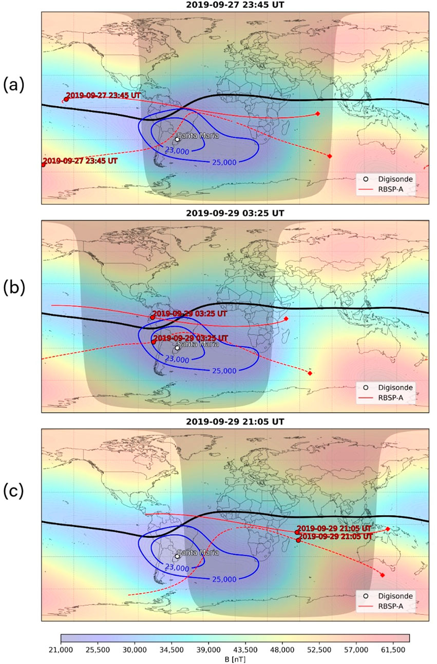
Figure 6. Maps of the geomagnetic field intensity evidencing the SAMA location in the region with the isointensity line of 25,000 nT. The location of Santa Maria Digisonde is marked by a white dot. The magnetic equator is shown by the black line. The RBSP orbit is represented by the continuous red line and its footprint in the dashed red line: (A) September 27, 2019, 23:45 UT, (B) September 29, 2019, 03:45 UT, and (C) September 29, 2019, 21:05 UT. The lengths of red lines represent the time interval in which the HSEs layers were detected in the Santa Maria Digisonde.

Figure 6 shows the SAMA identified as being the wide region inside the isointensity line of 25,000 nT. The Santa Maria Digisonde (white dot) is in the region of geomagnetic field intensity lower than 23,000 nT. The RBSP orbit’s locations during the occurrences of HSEs layers are represented by the continuous red line, while its footprint is shown by the dashed red line. The length of these lines corresponds to the period in which the HSEs layers were detected over Santa Maria. Therefore, the plasma wave dynamics can be studied during the period of HSEs layers’ occurrences. For instance, Figure 6A shows the RBSP location (red dot) on 27 September 2019, at 23:45 UT, when the ionogram from Figure 1B was collected. This ionogram is from the event that started at 22:20 UT on September 27 and finished at 2:20 UT on September 28, lasting 1 h 35 min. This period is named “Event A.” It is important to emphasize that what matters here is that the RBSP passes through the SAMA during the occurrence of the HSEs layers to observe plasma waves in the plasmasphere. It doesn’t have to be exactly at the same time. Figure 6B show the RBSP orbit when the HSEs layer observed in Figure 1C occurred. Similarly, Figure 6C show the RBSP orbit during the second and third events of HSEs layers and are named “Event B” and “Event C,” respectively. “Event B” occurred from 2:50 to 5:35 UT on September 29 and an ionogram taken during this time interval is shown in Figure 1C. “Event C” occurred from 20:10 to 22:30 UT on the same day, September 29, and a selected ionogram from this event is shown in Figure 1D.

On 27 September 2019, a geomagnetic storm was caused by a disturbed solar wind field associated with HSS from the coronal hole CH65+, as reported by the Database of Notifications, Knowledge, Information (DONKI) repository. The solar wind parameters (proton density–Np (a), solar wind speed–Vsw (b), and IMF Bz (c) component) and indexes AE (d) and SYM/H (e) from September 27 to 30, 2019 are shown in Figure 7. On September 27, Np exhibited an abrupt increase from ∼5 to ∼45 proton cm-³ around 10:30 UT, decreasing subsequently to values lower than 5 cm⁻³ along of the next 3 days. Vsw also increased from ∼350 km/s to ∼700 km/s at 22:00 UT on September 27. The intensity varied close to 650 km/s in the next day, September 28, and decreased to 500–400 km/s on the course of the following 2 days. The IMF Bz oscillated between ±10 nT during the incidence of HSS on September 27 and remained around ±5 nT in the course of September 28–30. Note that the IMF Bz remained predominantly negative from 12:00 to 23:00 UT on September 27. The AE index values exhibited several peaks during the whole period of analysis. Some of them, as on September 27 and 28, achieved more than 1,000 nT. At 9:00 UT on September 28, AE peaked at ∼2,000 nT. Before the HSS arrives, the SYM/H index was observed close to zero. At around 6:00 UT on September 27, the storm commencement was observed to occur, and the SYM/H values increased to 25 nT. In the following, the main phase started around 10:30 UT and lasted at 23:08 UT on September 27 when the SYM/H achieved −61 nT. After 23:08 UT, the recovery phase started for a few days. In this period, SYM/H remained at negative values between −10 and −40 nT and Kp index de-creased from 5+ to 4-. The red rectangles in Figure 7 show the periods of the Events “A”, “B”, and “C”.

Figure 7

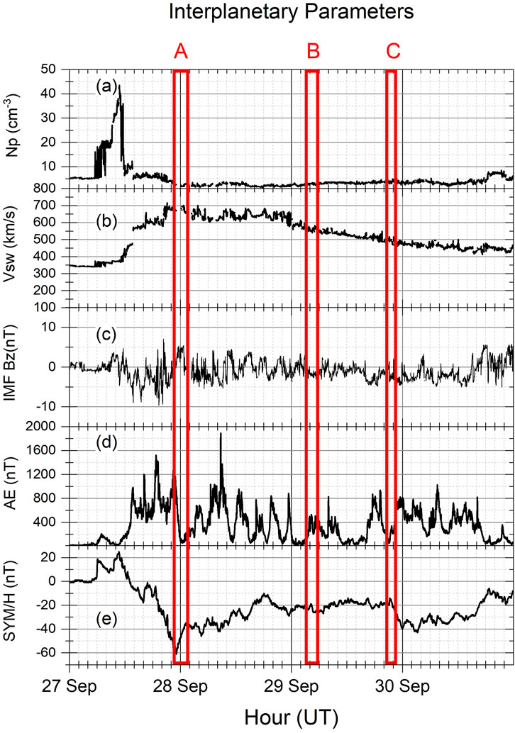
Figure 7. Interplanetary parameters: (A) Protons density, (B) solar wind speed, (C) Interplanetary Magnetic Field Bz Component, and indexes (D,E) SYM-H during the September 27, 2019, geomagnetic storm. The red rectangle shows the three events where the HSEs layers were observed.

The Events “A”, “B”, and “C” occurred during the main and recovery phases of the geomagnetic storm. To investigate the plasma wave dynamics in the inner radiation belt during these periods, the power spectral density of the magnetic field provided by the EMFISIS instrument onboard the RBSP is presented in Figure 8. The black lines represent the electron density (units changed from cm^-3 to Hz). The UT, L-shells parameter, and Magnetic Local Time (MLT) are shown in the ‘x’ axis (note that the RBSP orbits during these periods are shown in Figure 6).

Figure 8

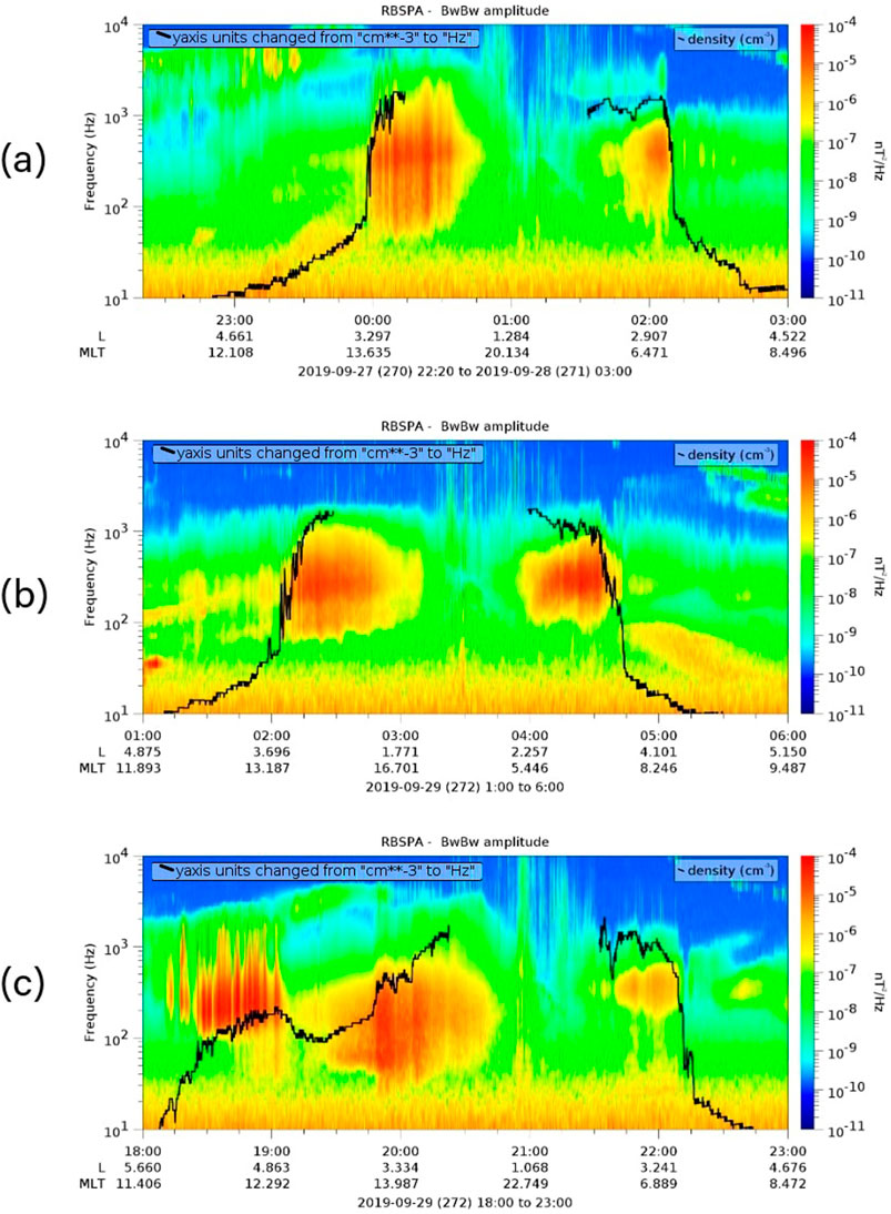
Figure 8. (A–C) Frequency-time spectrogram of the Magnetic field intensity obtained from EMFISIS instrument onboard the RBSP. The black lines represent electron density (units changed from cm⁻³ to Hz).

In Figure 8, the most intense regions with power approximately 10–4 nT²/Hz show the plasmaspheric hiss wave activities in the slot and inner radiation belt. The main loss processes for inner belt electrons include pitch angle scattering driven by hiss and magnetosonic (MS) waves, and energy loss caused by collisions, both processes control the lifetime of the electrons (Selesnick, 2016), which can cause electron precipitation to the atmosphere. The process occurs during the bouncing movement of the charged particles, when they will reach minimum altitudes at the mirror points in both Northern and Southern Hemispheres. If a charge particle presents an equatorial pitch angle of α₀ in a field line with intensity B₀ there, the intensity of the magnetic field at the mirror point (B_mp) should be given by Equation 2 (Baumjohann and Treumann, 1996):

${\sin }^2\left({\mathrm{\alpha }}_0\right)=\frac{B_0}{B_{mp}}(2)$

Equation 2 shows that the lower intensity of the magnetic field in the SAMA region brings the mirror point of charge particles to lower heights. Charged particles with mirror points at ∼900 km in the Northern Hemisphere will present mirror points at ∼100 km in the SAMA (Abel and Thorne, 1999; Torr et al., 1975).

The inner belt dynamic under the influence of the geomagnetic storms can intensify the amplitude of the hiss waves, as observed in Figure 8. The interaction between hiss and MS waves with the increased number of charge particles can scatter and launch electrons (0.5 KeV to a few tens of keV) into flux tubes that pass through the SAMA region. Consequently, more electrons will be in the loss cone, penetrating in the E-region heights, and exciting the atoms and molecules (see Da Silva et al., 2022; Da Silva et al., 2023; Moro et al., 2022b; Resende et al., 2022a; Resende et al., 2022b).

The mechanism described above is the most likely process responsible for the HSEs layers during the Events “A” and “B”. In agreement with previous works, these HSEs layers can also be classified as Esa layers. The HSEs layer in Event “C”, Figure 1D, seems to be influenced by another mechanism in addition to electron precipitation. The evidence for this statement is the presence of a slant Es (Ess) layer at 21:05 UT, which is associated with the presence of gravity waves (Cohen et al., 1962). Since this geomagnetic storm was not intense, and September 29 is the last day of the recovery phase with AE index <400 nT in the period, it is possible that this second mechanism overlaps the first one during this interval. Future works need to include an analysis of gravity waves in similar cases to distinguish the main source of this type of echo from the E-region in such conditions.

Finally, the relationship between the HSEs layer occurrences and days with Kp > 3 is worth showing in Figure 9. This figure is composed basically of two lines. The first one shows the HSEs layer occurrences painted red. The second line corresponds to the period of 1 July 2019, to 30 June 2020. If at least one of the eight Kp values of the day is >3, the day is painted red. The days when occurred data gaps due to technical issues of the Digisonde are painted black. Otherwise, the days are left white if no HSEs layers were detected (first line) or if the day is classified as been geomagnetically quiet (second line). Figure 9 shows that the HSEs layers generally occurred during geomagnetically quiet conditions in the data set analysed in this work. Therefore, this result shows that is incorrect to attribute the spread echoes from the E-region detected in the SAMA as Esa layers. This find is a motivation to investigate the HSEs layer causes during geomagnetically quiet periods, which is performed in the next section.

Figure 9

Figure 9. Relationship between the HSEs layer occurrences (first line) with geomagnetic conditions (second line) from 1st July 2019, to 30th June 2020. In the first line, the occurrences of HSEs layers are highlighted in red, the data gaps in black, and left white when there are no occurrences of HSEs layers. In the second line, the geomagnetically disturbed (quiet) days are painted red (white).

3.4 HSEs layers during geomagnetically quiet conditions

The HSEs layers development during geomagnetic disturbed conditions, presented in the previous section, agrees with previous works about the importance of wave-particle interaction in the energetic particle precipitation in the SAMA. The HSEs layers, in these cases, may be classified as Esa layers. However, a question arises now when the HSEs layers are observed during geomagnetic quiet conditions: what is the physical mechanism responsible for their formation? Moreover, what is the OR of HSEs layers during quiet times and as a function of LT? Figure 10 is used to answer the second question. It shows the monthly and seasonal occurrence rates of the HSEs layers during geomagnetically quiet days. It follows the same pattern as Figure 4 that considers both geomagnetic quiet and disturbed days. Overall, the pattern remains similar, but the OR decreases in all months except in May, as seen in Figure 10A. The exception occurs because Mays presents only two geomagnetic disturbed days with Kp = 3+ (days 6 and 30), and these 2 days did not show the development of HSEs layers. The most significant OR decreases of HSEs layers occurred in September (32%), February (26%), and August (23%). These months presented the highest numbers of geomagnetic disturbed data collected by the Santa Maria Digisonde. This is also reflected in Figure 10B.

Figure 10

Figure 10. (A) Monthly and (B) seasonal occurrence rates of spread echoes from the E-region considering geomagnetically quiet conditions.

Interestingly, very few cases of HSEs layers started during daytime in geomagnetically disturbed conditions in the data set analyzed here: (i) 12:55–16:00 UT on January 9 (Kp = 4-); (ii) 9:55–12:10 UT on February 19 (Kp = 4); (iii) 11:15–12:15 UT on March 30 (Kp = 4). Therefore, the OR patterns presented in Figures 2, 3 (that consider both geomagnetic quiet and disturbed days) remain almost the same. Put differently, versions of Figures 2, 3 considering only geomagnetically quiet data are not shown because the estimate OR decreases is lower than 1% for daytime hours in these three cases.

To answer the first question raised in this section, which is about the physical mechanism responsible for the HSEs layers formation during quiet times, Digisonde and the RBSP data are used again. It is considered RBSP data obtained during the perigee orbit over the SAMA when HSEs layer events were observed in the ionograms in Figures 1E–H. Figure 11 shows the power spectral density of the magnetic field, in which the plasmaspheric hiss wave activities in the slot and inner radiation belt are observed similarly as to those in Figure 8. However, the amplitude of these hiss waves is considerably low, approximately two-three orders of magnitude less than the geomagnetic storm period (e.g., Da Silva et al., 2022; Da Silva et al., 2023; Moro et al., 2022a). Therefore, it is plausible that other mechanisms are operating during the occurrences of the HSEs layers of Figures 1E–H, which present ftEs values similar to the HSEs layers during geomagnetically disturbed conditions.

Figure 11

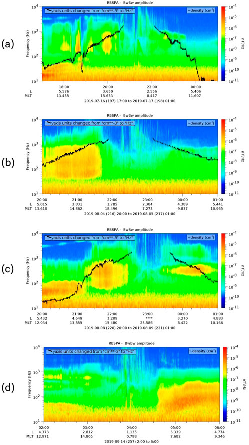
Figure 11. (A–D) Same as Figure 8, but during geomagnetic quiet conditions.

One of the suggested mechanism responsible for the HSEs layers in Figures 1E–H, with low ftEs, is the Cosmic Ray Albedo Neutron Decay (CRAND), which is known to govern the inner radiation belt dynamic during quiet periods and is an important source of populating the inner belt electrons (Li et al., 2017; Zhang et al., 2019). Therefore, during the quiet-time period, the electron injections by CRAND processes can occur in the inner radiation belt with different lifetimes, with the lifetime (t) shorter than one bounce period (t_b) (t < t_b to precipitate), longer than one bounce period but shorter than one drift period (t_d) (t_d < t < t_b, quasitrapped), and longer than one drift period (t > t_d, trapped) (Zhang et al., 2019). These conditions suggest that the electrons with the first and second type of lifetime injected through the CRAND processes can precipitate into the atmosphere during the quiet period, even with low hiss wave amplitude, contributing in this way to the generation of the HSEs layers over the SAMA region without the presence of the geomagnetic storms.

A second mechanism suggested here is the instabilities such as KHI (Choudhary et al., 2005; Larsen, 2000). This mechanism can operate independently of the geomagnetic conditions and during daytime as well, i.e., also explaining the HSEs layers presented in Figures 1I–L. Radar data obtained in middle latitudes showed that winds with large amplitudes and gravity waves developed the KHI, causing very spread echoes from the E-region (Chen et al., 2020; Yan et al., 2022). Resende et al. (2023) studied, for the first time, the spreading Es layers over Cachoeira Paulista observed during geomagnetically quiet times. The authors used several measuring techniques such as all-sky imager, satellite and meteor radar data to understand the mechanism behind the phenomena. The explanation given by the authors is based on instabilities due to turbulent winds and/or gravity waves in the Es layer formation. In one case study, the authors found the presence of gravity waves in the OH images concomitant with the Ess layer at 23:15 UT on 6 May 2018. In this case, the gravity wave could grow instability and cause the observed spread Es layer over the station.

Unfortunately, radar data, airglow images, and wind data are not available in the Santa Maria region during the HSEs layers presented in Figures 1E–L. However, analysis of the plasma density gradient variations (ΔfEs) gives the Es layer structure (Chen et al., 2020; Fahrutdinova et al., 1997; Moro et al., 2022a) and can indicate the presence of irregularities in the E-region. The parameter ΔfEs is calculated by the difference between the ftEs and the blanketing frequency (fbEs) of Es layers. Fahrutdinova et al. (1997) explains that peaks of ΔfEs are attributed to the mesoscale turbulence in the lower thermosphere, and Ogawa et al. (1998) showed that peaks in ΔfEs correlate well with the quasiperiodic radar echoes observed in the middle latitude.

The ΔfEs from manually scaled ftEs and fbEs parameters are shown in Figure 12A for the days in which the ionograms of Figures 1E–H were collected: 16 July (black line), 4 August (red line), 8 August (blue line), and 14 September (green line). It is noticed that the ΔfEs parameters do not show significant increases during the HSEs layers occurrences. Indeed, 16 July is the parameter with higher increases, but the value of ΔfEs is lower than 3 MHz. However, Figure 12B shows the ΔfEs variations calculated for the days in which the ionograms of Figures 1I–L were obtained: 16 November (black line), 9 January (red line), 12 January (blue line), and 30 March (green line). It is clear that the days in which the HSEs layers occurred during daytime presented very intense oscillations. For instance, on 16 November the ΔfEs achieved more than 5 MHz at around 13:30 UT, when the HSEs layer was observed in Figure 1I. Therefore, the intense peaks observed in the ΔfEs in Figure 12B are evidence that the wind-shear mechanism is turbulent during the daytime ionograms with HSEs layers. Contrary, it is also observed that on 30 March 2020, Figure 1L, when the HSEs layer is weak (ftEs ∼4 MHz), the time-variation of ΔfEs is smoother. In this case, the CRAND mechanism could be involved. Finally, it is believed that the instabilities could be responsible for the HSEs layers of Figures 1I–K, which present higher ftEs compared to the HSEs layers of Figures 1E–H, which might be caused by CRAND mechanism. However, future research on this topic is very important to elucidate the mechanism that acted in these cases. Recently, an all-sky imager and a meteor radar were installed close to Santa Maria station and can help to understand the origin of nighttime and daytime HSEs layers during geomagnetically quiet periods.

Figure 12

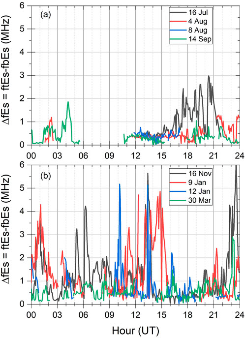
Figure 12. (A,B) Variations of the plasma density gradient variations (ΔfEs = ftEs–fbEs) recorded by the Santa Maria Digisonde. ftEs is the top frequency and fbEs is the blanketing frequency of the sporadic-E (Es) layer.

4 Conclusion

In this study, the spread echoes from the E-region detected in ionograms collected in the South American Magnetic Anomaly (SAMA) region are classified for the first time as “Height-Spread Es (HSEs) layers.” The HSEs layers start at around 100 km altitude and have a thickness of around 30–50 km, or more in some cases, with the Esf (nighttime) or Esl (daytime) Es in the background (typical blanketing Es (Esb) layer types caused by the wind-shear mechanism). This work also provides the first statistical analysis of HSEs layers. Their occurrence rates over the Santa Maria station, Brazil, is 9.8%, based on Digisonde data collected from July 2019 to June 2020. Occurrence rates over several time intervals (hours, months, seasons) are also presented. The highest occurrence rates were observed in November, December, and January.

HSEs layers are classified based on geomagnetic conditions. They occurred mainly during geomagnetically quiet conditions and were predominantly observed during nighttime, with some events also detected during daytime. The top frequency (ftEs) of HSEs layers is generally lower at night compared to daytime. The temporal evolution of HSEs traces is irregular, similar to that of Esb layers.

During the 27 September 2019, geomagnetic storm, the HSEs layers could also be classified as Esa layers, as electron precipitation was the most likely mechanism for its origin, as indicated by the observation of hiss waves in the inner radiation belt. On the other hand, during geomagnetically quiet conditions, two potential mechanisms are suggested for the HSEs layers formation: (i) the CRAND mechanism, which would produce HSEs layers with lower ftEs, and (ii) the Kelvin-Helmholtz Instability (KHI), which would produce the daytime HSEs layers with high ftEs values (sometimes exceeding 9 MHz). This is supported by the significant peaks in plasma density gradient variations (ΔfEs) during daytime compared to nighttime. However, the presence of Ess layers during nighttime also suggests the development of KHI after sunset.

Future studies incorporating data from all-sky imager and meteor radar recently installed near the Santa Maria station will provide deeper insights into the physical mechanisms behind the formation of HSEs layers, particularly under geomagnetically quiet conditions.

Data availability statement

The original contributions presented in the study are included in the article/supplementary material, further inquiries can be directed to the corresponding author.

Author contributions

JM: Conceptualization, Data curation, Formal Analysis, Investigation, Methodology, Software, Validation, Writing–original draft, Writing–review and editing. JX: Supervision, Writing–review and editing. JB: Supervision, Writing–review and editing. LdS: Conceptualization, Formal Analysis, Investigation, Software, Writing–review and editing. LR: Writing–review and editing, Conceptualization. CD: Writing–review and editing. VA: Writing–review and editing. AS: Writing–review and editing. GP: Writing–review and editing. HL: Writing–review and editing, Funding acquisition, Project administration, Resources. LZ: Funding acquisition, Project administration, Resources, Writing–review and editing. CW: Funding acquisition, Project administration, Resources, Writing–review and editing. NS: Writing–review and editing.

Funding

The author(s) declare that financial support was received for the research, authorship, and/or publication of this article. This work is supported by the International Partnership Program of Chinese Academy of Sciences, Grants 183311KYSB20200017 and 183311KYSB20200003.

Acknowledgments

JM, LdS, LR, VA, and AS would like to thank the China-Brazil Joint Laboratory for Space Weather (CBJLSW), National Space Science Center (NSSC), and the Chinese Academy of Science (CAS) for supporting their postdoctoral fellowship. CD thanks the CNPq through Grant 302675/2021-3. GP extends sincere thanks to the São Paulo Research Foundation (FAPESP) for financial support through Grant 2023/07518-7.

Conflict of interest

The authors declare that the research was conducted in the absence of any commercial or financial relationships that could be construed as a potential conflict of interest.

Generative AI statement

The author(s) declare that no Generative AI was used in the creation of this manuscript.

Publisher’s note

All claims expressed in this article are solely those of the authors and do not necessarily represent those of their affiliated organizations, or those of the publisher, the editors and the reviewers. Any product that may be evaluated in this article, or claim that may be made by its manufacturer, is not guaranteed or endorsed by the publisher.

References

Abel, B., and Thorne, R. M. (1999). Modeling energetic electron precipitation near the South Atlantic Anomaly. J. Geophys. Res. Space Phys. 104 (A4), 7037–7044. doi:10.1029/1999JA900023

CrossRef Full Text | Google Scholar

Batista, I. S., and Abdu, M. A. (1977). Magnetic storm associated delayed sporadic E enhancements in the Brazilian Geomagnetic Anomaly. J. Geophys. Res. Space Phys. 82, 4777–4783. doi:10.1029/ja082i029p04777

CrossRef Full Text | Google Scholar

Baumjohann, W., and Treumann, R. A. (1996). Basic space plasma physics. London: ICP.

Google Scholar

Bernhardt, P. A. (2002). The modulation of sporadic-E layers by Kelvin–Helmholtz billows in the neutral atmosphere. J. Atmos. Solar-Terrestrial Phys. 64 (12), 1487–1504. doi:10.1016/S1364-6826(02)00086-X

CrossRef Full Text | Google Scholar

Cameron, T., Fiori, R., Themens, D., Warrington, E., Thayaparan, T., and Galeschuk, D. (2022). Evaluation of the effect of sporadic-E on high frequency radio wave propagation in the arctic. J. Atmos. Solar-Terrestrial Phys. 228, 105826. doi:10.1016/j.jastp.2022.105826

CrossRef Full Text | Google Scholar

Chen, G., Wang, Z., Jin, H., Yan, C., Zhang, S., Feng, J., et al. (2020). A case study of the daytime intense radar backscatter and strong ionospheric scintillation related to the low-latitude E-region irregularities. J. Geophys. Res. Space Phys. 125 (7), e2019JA027532. doi:10.1029/2019JA027532

CrossRef Full Text | Google Scholar

Choudhary, R. K., St.-Maurice, J.-P., Kagan, L. M., and Mahajan, K. K. (2005). Quasi-periodic backscatters from the E region at Gadanki: evidence for Kelvin-Helmholtz billows in the lower thermosphere? J. Geophys. Res. Space Phys. 110 (A8). doi:10.1029/2004JA010987

CrossRef Full Text | Google Scholar

Cohen, R., Bowles, K. L., and Calvert, W. (1962). On the nature of equatorial slant sporadic E. J. Geophys. Res. (1896-1977) 67 (3), 965–972. doi:10.1029/JZ067i003p00965

CrossRef Full Text | Google Scholar

Da Silva, L. A., Shi, J., Resende, L. C. A., Agapitov, O. V., Alves, L. R., Batista, I. S., et al. (2022). The role of the inner radiation belt dynamic in the generation of auroral-type sporadic E-layers over south American magnetic anomaly. Front. Astronomy Space Sci. 9. doi:10.3389/fspas.2022.970308

CrossRef Full Text | Google Scholar

Da Silva, L. A., Shi, J., Vieira, L. E., Agapitov, O. V., Resende, L. C. A., Alves, L. R., et al. (2023). Why can the auroral-type sporadic E layer be detected over the South America Magnetic Anomaly (SAMA) region? An investigation of a case study under the influence of the high-speed solar wind stream. Front. Astronomy Space Sci. 10. doi:10.3389/fspas.2023.1197430

CrossRef Full Text | Google Scholar

Denardini, C. M., Abdu, M. A., de Paula, E. R., Sobral, J. H. A., and Wrasse, C. M. (2005). Seasonal characterization of the equatorial electrojet height rise over Brazil as observed by the RESCO 50 MHz back-scatter radar. J. Atmos. Sol. Terr. Phys. 67 (17–18), 1665–1673. doi:10.1016/j.jastp.2005.04.008

CrossRef Full Text | Google Scholar

Fahrutdinova, A. N., Sherstyukov, O. N., and Yasnitsky, D. S. (1997). The influence of the mesoscale turbulence in lower thermo-sphere-upper mesosphere on the mid-latitude sporadic E-layer. Adv. Space Res. 20 (6), 1305–1307. doi:10.1016/S0273-1177(97)00792-8

CrossRef Full Text | Google Scholar

Gonzalez, W. D., Dutra, S. L. G., and Pinto, O. (1987). Middle atmospheric electrodynamic modification by particle precipitation at the South Atlantic Magnetic Anomaly. J. Atmos. Terr. Phys. 49 (4), 377–383. doi:10.1016/0021-9169(87)90032-8

CrossRef Full Text | Google Scholar

Haldoupis, C. (2011). “A tutorial review on sporadic E layers,” in Aeronomy of the Earth’s atmosphere and ionosphere. Editors M. A. Abdu, and D. Pancheva (Dordrecht: Springer Netherlands), 381–394. doi:10.1007/978-94-007-0326-1_29

CrossRef Full Text | Google Scholar

Jayanthi, U. B., Pereira, M. G., Martin, I. M., Stozkov, Y., D’Amico, F., and Villela, T. (1997). Electron precipitation associated with geomagnetic activity: balloon observation of X ray flux in South Atlantic anomaly. J. Geophys. Res. Space Phys. 102 (A11), 24069–24073. doi:10.1029/97JA01817

CrossRef Full Text | Google Scholar

Larsen, M. F. (2000). A shear instability seeding mechanism for quasiperiodic radar echoes. J. Geophys. Res. Space Phys. 105 (A11), 24931–24940. doi:10.1029/1999JA000290

CrossRef Full Text | Google Scholar

Li, X., Selesnick, R., Schiller, Q., Zhang, K., Zhao, H., Baker, D. N., et al. (2017). Measurement of electrons from albedo neutron decay and neutron density in near-Earth space. Nature 552 (7685), 382–385. doi:10.1038/nature24642

PubMed Abstract | CrossRef Full Text | Google Scholar

Mathews, J. D. (1998). Sporadic E: current views and recent progress. J. Atmos. Solar-Terrestrial Phys. 60 (4), 413–435. doi:10.1016/S1364-6826(97)00043-6

CrossRef Full Text | Google Scholar

Mauk, B. H., Fox, N. J., Kanekal, S. G., Kessel, R. L., Sibeck, D. G., and Ukhorskiy, A. (2013). Science objectives and rationale for the radiation belt storm Probes mission. Space Sci. Rev. 179 (1), 3–27. doi:10.1007/s11214-012-9908-y

CrossRef Full Text | Google Scholar

McNamara, L. F. (1991). The ionosphere: communications, surveillance, and direction finding. Malabar, Florida: Krieger publishing company.

Google Scholar

Moro, J., Denardini, C. M., Resende, L. C. A., Chen, S. S., and Schuch, N. J. (2016). Equatorial E region electric fields at the dip equator: 1. Variabilities in eastern Brazil and Peru. J. Geophys. Res. Space Phys. 121 (10), 220–310. doi:10.1002/2016JA022751

CrossRef Full Text | Google Scholar

Moro, J., Xu, J., Bageston, J. V., Denardini, C. M., Andrioli, V. F., Resende, L. C. A., et al. (2023). Analysis of blanketing sporadic-E layer and associated tidal periodicities over a Brazilian station undergoing a transition from low latitude to mid-latitude. J. Geophys. Res. Space Phys. 128 (12), e2023JA031947. doi:10.1029/2023JA031947

CrossRef Full Text | Google Scholar

Moro, J., Xu, J., Denardini, C. M., Resende, L. C. A., Da Silva, L. A., Chen, S. S., et al. (2022b). Different sporadic-E (Es) layer types development during the August 2018 geomagnetic storm: evidence of auroral type (Esa) over the SAMA region. J. Geophys. Res. Space Phys. 127 (2), e2021JA029701. doi:10.1029/2021JA029701

CrossRef Full Text | Google Scholar

Moro, J., Xu, J., Denardini, C. M., Resende, L. C. A., Silva, R. P., Liu, Z., et al. (2019). On the sources of the ionospheric variability in the South American magnetic anomaly during solar minimum. J. Geophys. Res. Space Phys. 124 (9), 7638–7653. doi:10.1029/2019JA026780

CrossRef Full Text | Google Scholar

Moro, J., Xu, J., Denardini, C. M., Stefani, G., Resende, L. C. A., Santos, A. M., et al. (2022a). Blanketing sporadic-E layer occurrences over Santa Maria, a transition station from low to middle latitude in the South American magnetic anomaly (SAMA). J. Geophys. Res. Space Phys. 127 (12), e2022JA030900. doi:10.1029/2022JA030900

CrossRef Full Text | Google Scholar

Ogawa, T., Sekito, N., Nozaki, K., and Yamamoto, M. (1998). Height comparison of midlatitude E region field-aligned irregularities and sporadic E Layer. Geophys. Res. Lett. 25 (11), 1813–1816. doi:10.1029/98GL00864

CrossRef Full Text | Google Scholar

Piggott, W. R., and Rawer, K. (1978). U.R.S.I. Handbook of ionogram interpretation and reduction (23A). Boulder, Colorado: World Data Center A for Solar-Terrestrial Physics, NOAA, 146. Available at: https://repository.library.noaa.gov/view/noaa/10404.

Google Scholar

Pinto, Jr. O., and Gonzalez, W. D. (1986). X ray measurements at the South atlantic magnetic anomaly. J. Geophys. Re-search Space Phys. 91 (A6), 7072–7078. doi:10.1029/JA091iA06p07072

CrossRef Full Text | Google Scholar

Resende, L. C. A., Zhu, Y., Arras, C., Denardini, C. M., Chen, S. S., Moro, J., et al. (2022a). Analysis of the sporadic-E layer behavior in different American stations during the days around the september 2017 geomagnetic storm. Atmosphere 13 (10), 1714. doi:10.3390/atmos13101714

CrossRef Full Text | Google Scholar

Resende, L. C. A., Zhu, Y., Denardini, C. M., Chagas, R. A. J., Da Silva, L. A., Andrioli, V. F., et al. (2023). Analysis of the different physical mechanisms in the atypical sporadic E (Es) layer occurrence over a low latitude region in the Brazilian sector. Front. Astronomy Space Sci. 10. doi:10.3389/fspas.2023.1193268

CrossRef Full Text | Google Scholar

Resende, L. C. A., Zhu, Y., Denardini, C. M., Moro, J., Da Silva, L. A., Arras, C., et al. (2022b). Worldwide study of the Sporadic E (Es) layer development during a space weather event. J. Atmos. Solar-Terrestrial Phys. 241, 105966. doi:10.1016/j.jastp.2022.105966

CrossRef Full Text | Google Scholar

Seif, A., Liu, J.-Y., Mannucci, A. J., Carter, B. A., Norman, R., Caton, R. G., et al. (2017). A study of daytime L-band scintillation in association with sporadic E along the magnetic dip equator. Radio Sci. 52, 1570–1577. doi:10.1002/2017RS006393

CrossRef Full Text | Google Scholar

Seif, A., and Panda, S. K. (2024). Characterizing global equatorial sporadic-E layers through COSMIC GNSS radio occultation measurements. Astrophysics Space Sci. 369, 60. doi:10.1007/s10509-024-04326-2

CrossRef Full Text | Google Scholar

Selesnick, R. S. (2016). Stochastic simulation of inner radiation belt electron decay by atmospheric scattering. J. Geophys. Res. Space Phys. 121 (2), 1249–1262. doi:10.1002/2015JA022180

CrossRef Full Text | Google Scholar

Thayaparan, T., and MacDougall, J. (2005). Evaluation of ionospheric sporadic-E clutter in an Arctic environment for the assessment of high-frequency surface-wave radar surveillance. IEEE Trans. Geosci. Rem. Sens. 43 (5), 1180–1188. doi:10.1109/tgrs.2005.844661

CrossRef Full Text | Google Scholar

Torr, D. G., Torr, M. R., Walker, J. C. G., and Hoffman, R. A. (1975). Particle precipitation in the South atlantic geomagnetic anomaly. Planet. Space Sci. 23 (1), 15–26. doi:10.1016/0032-0633(75)90064-1

CrossRef Full Text | Google Scholar

Tsurutani, B. T., Smith, E. J., and Thorne, R. M. (1975). Electromagnetic hiss and relativistic electron losses in the inner zone. J. Geophys. Res. (1896-1977) 80 (4), 600–607. doi:10.1029/JA080i004p00600

CrossRef Full Text | Google Scholar

Vankadara, R. K., Panda, S. K., Amory-Mazaudier, C., Fleury, R., Devanaboyina, V. R., Pant, T. K., et al. (2022). Signatures of equatorial plasma bubbles and ionospheric scintillations from magnetometer and GNSS observations in the Indian longitudes during the space weather events of early september 2017. Remote Sens. 14, 652. doi:10.3390/rs14030652

CrossRef Full Text | Google Scholar

Whitehead, J. D. (1961). The formation of the sporadic-E layer in the temperate zones. J. Atmos. Terr. Phys. 20 (1), 49–58. doi:10.1016/0021-9169(61)90097-6

CrossRef Full Text | Google Scholar

Yan, C., Chen, G., Wang, Z., Zhang, M., Zhang, S., Li, Y., et al. (2022). Statistical characteristics of the low-latitude E-region irregularities observed by the HCOPAR in south China. J. Geophys. Res. Space Phys. 127 (1), e2021JA029972. doi:10.1029/2021JA029972

CrossRef Full Text | Google Scholar

Yu, B., Scott, C. J., Xue, X., Yue, X., and Dou, X. (2020). Derivation of global ionospheric Sporadic E critical frequency (fo Es) data from the amplitude variations in GPS/GNSS radio occultations. R. Soc. Open Sci. 7, 200320. doi:10.1098/rsos.200320

PubMed Abstract | CrossRef Full Text | Google Scholar

Yue, X., Schreiner, W. S., Pedatella, N. M., and Kuo, Y.-H. (2016). Characterizing GPS radio occultation loss of lock due to ionospheric weather. Space weather. 14, 285–299. doi:10.1002/2015SW001340

CrossRef Full Text | Google Scholar

Zeng, Z., and Sokolovskiy, S. (2010). Effect of sporadic E clouds on GPS radio occultation signals. Geophys. Res. Lett. 37. doi:10.1029/2010GL044561

CrossRef Full Text | Google Scholar

Zhang, K., Li, X., Zhao, H., Schiller, Q., Khoo, L.-Y., Xiang, Z., et al. (2019). Cosmic ray albedo neutron decay (CRAND) as a source of inner belt electrons: energy spectrum study. Geophys. Res. Lett. 46 (2), 544–552. doi:10.1029/2018GL080887

CrossRef Full Text | Google Scholar

Zhang, Y., Wu, J., Guo, L., Hu, Y., Zhao, H., and Xu, T. (2015). Influence of solar and geomagnetic activity on sporadic-E layer over low, mid and high latitude stations. Adv. Space Res. 55 (5), 1366–1371. doi:10.1016/j.asr.2014.12.010

CrossRef Full Text | Google Scholar