The March and April 2023 ionospheric storms over Europe

This paper presents a deep and comprehensive multi-instrumental analysis of two distinct ionospheric storms occurring in March and April 2023. We investigate the ionospheric response in the middle-latitudinal European region utilizing ionospheric vertical sounding at five European stations: Juliusruh, Dourbes, Pruhonice, Sopron, and a reference station, San Vito. Additionally, we employ Digisonde Drift Measurement, Continuous Doppler Sounding System, local geomagnetic measurements, and optical observations. We concentrate on the F2 and F1 region parameters and shape of the electron density profile. During the March event, a pre-storm enhancement was observed, characterized by an increase in electron density up to approximately 20% at northern stations, with minimal effect observed at San Vito. We present a novel detailed temporal and spatial description of a so-called G-condition. It was observed not only in the morning hours in the period of the increased geomagnetic activity during (and shortly after) the main phase of the storm, but also during low to moderate geomagnetic activity with Kp between 1 and 3+. Further, an alteration in the shape of the electron density profile, notably captured by the parameter B0 was observed. A substantial increase in B0, by several hundred percent, was noted during both events on the day of the geomagnetic disturbance and importantly also on the subsequent day with low-to-moderate geomagnetic activity. During both storms, the critical frequency foF1 decreased at all stations including San Vito. Changes in electron density in the F1 region indicate plasma outflow during morning hours. Distinct and persistent oblique reflections from the auroral oval were observed on the ionograms for several hours during both events and these observations were in agreement with optical observations of auroral activity and concurrent rapid geomagnetic changes at collocated stations. For the first time, we present a unique and convincing excellent agreement between the Continuous Doppler Sounding System and Digisonde Drift Measurement. The results reveal vertical movement of plasma up to ±80 m/s. Analysis of observed vertical plasma drifts and horizontal component H of magnetic field in Czechia and Belgium suggest that vertical motion of the F-region plasma is caused by ExB plasma drift.

1 Introduction

Solar activity stands as the primary driver of ionospheric disturbances, a phenomenon under study since the early 20th century, notably through the pioneering works of Hafstad and Tuve (1929) and Appleton and Ingram (1935). Comprehensive reviews on ionospheric storms can be found in Buonsanto (1999) and Prölss (1995), among others. Solar activity predictions play a crucial role in various operational planning endeavors, such as satellite lifespan estimations in low-Earth orbit, radiation exposure anticipation for ongoing and forthcoming missions, and contingency preparations for radio-based communication and navigation systems outages (Pesnell, 2008; Kodikara et al., 2021; Rejfek et al., 2023).

Overview on the typical ionospheric storm behavior over Europe for the period between 1996 and 2013 during SC 23 and beginning of SC 24 is given in Borries et al. (2015). Efforts to analyze and forecast solar activity for Solar Cycle 25 (SC 25) have been extensive (e.g., McIntosh et al., 2020), drawing on observations from previous solar cycles, notably the unusually deep and prolonged minimum between SC 23 and SC 24 (Lockwood et al., 2012). In this context an important issue arises as the estimation of the level of solar activity by only one index (usually by the sunspot number) does not fully describe the impact of solar activity on the Earth (Georgieva et al., 2012).

Forecasts for SC 25 have varied widely, with many suggesting it to be comparatively weaker than its predecessors. However, current observations reveal that though at the time of this writing SC 25 has not yet reached its maximum, solar activity during SC 25 seems to be at least comparable or even somewhat higher than during SC 24. The ionospheric effects observed thus far in SC 25 have been the most substantial to date, with geomagnetic activity severity comparable to the largest events witnessed in the preceding solar cycle (e.g., Blagoveshchensky and Sergeeva, 2019; Berdermann et al., 2018). The recent Mother’s Day superstorm in May 2024 (promptly analyzed for the Mediterranean region by Spogli et al., 2024) exemplifies the critical need for comprehensive studies on the effects of space weather on the geosphere. This event underscores the likelihood of future solar-induced events significantly impacting the ionosphere during Solar Cycle 25.

There were many excellent storm studies from the solar cycle 24 examining the Northern hemisphere and the European region, see study of Blagoveshchensky and Sergeeva (2019); Berdermann et al. (2018), Nayak et al. (2016), Nava et al. (2016), Astafyeva et al. (2015), Berényi et al. (2018, 2023), Mosna et al. (2020), Oikonomou et al. (2022). As a main conclusion of these papers was that during intense geomagnetic storm events (Dstmin < −100 nT) with analysis of multi-instrument data like Digisonde ionospheric parameters and drift data, satellite measurements like Swarm, TIMED, GNSS etc., the evolution of the solar-induced ionospheric storm features like TIDs (Travelling Ionospheric Disturbances), MIT (Midlatitude ionospheric trough, which is the ionospheric footprint of the plasmapause, see Heilig et al., 2022) etc. can be tracked well. Besides, they also highlighted the importance of Prompt Penetration Electric fields (PPEFs) and Disturbance Dynamo Electric Fields (DDEFs) during the progress of the ionospheric storms.

Sources of TIDs in the ionosphere are subject of both theoretical and experimental studies. Fundamental theory of atmospheric gravity waves (AGW), traveling atmospheric disturbances (TAD) and their imprints observed as TIDs within the ionospheric plasma has been provided by Hines (1960) and later developed in works by Chimonas and Hines (1970), Hooke (1968) and many others. Hunsucker (1982), Hocke and Schlegel (1996) provided review of TIDs associated with auroral sources. An expansion due to heating in the thermosphere during geomagnetic disturbance leads to a generation and propagation of a wave-like structures in the form of TADs, and consequently also in the form of TIDs (Prolss, 2012; Shiokawa et al., 2007; Kim et al., 2023; Buonsanto, 1999 and others). Besides the TIDs related to geomagnetic disturbances the ionosphere is influenced by acoustic gravity waves (see e.g., Figure 1 in Astafyeva, 2019) originating in the lower and middle atmosphere (for instance Koucká Knížová et al., 2021; Laštovička, 2006; Kazimirovsky, 2002 and others), however the storm associated TIDs are generally considered to be more intense than those observed in connection to neutral lower-lying atmosphere sources. Study Kishore and Kumar (2023) demonstrates that the morphology of TIDs parameters continually varies over time due to highly dynamic ionospheric response to geomagnetic storms. Their study indicated possible resonating effects at middle and low latitude stations. The observed TID response for two comparable superstorms is significantly different owing to the differing storm evolution patterns.

Figure 1

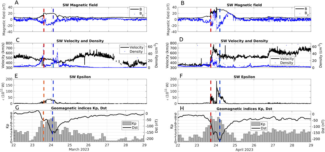
Figure 1. Solar activity (left panels for March 2023, right panels for April 2023) by means of B, Bz (A, B), solar wind velocity and density (C, D), solar wind epsilon parameter (E, F), and geomagnetic indices Kp and Dst (G, H). Left dashed red lines in each panel denote SSC (23 March, 14:11 UT and 23 April, 17:35 UT). Right dashed blue lines denote minimum of Dst (24 March, 03:00 UT, 24 April, 05:00).

Recent studies on the March and April storms, primarily based on Global Navigation Satellite System (GNSS) derived Total Electron Content (TEC), have been published. Tariq et al. (2024) presented longitudinal variations in the American and Asian sectors based on GNSS observations. Rajana et al. (2024) analyzed the Indian sector for the March and April storm. Data from GNSS stations and FORMOSAT-7/COSMIC-2 occultation observations reveal rapid changes in TEC Rate of TEC Index (ROTI) during the April storm in equatorial and low-latitude regions (Wang et al., 2023). Paul et al. (2024) analyzed parameters from the F2 region and TEC over Europe during March 2023 and concluded that the storm effects were dependent on the location of the stations with more pronounced changes at northern located stations, most significantly at Juliusruh. In their study, Pancheva et al. (2024) present global behavior of the ionospheric TEC peculiarities during a geomagnetic storm in March 2023. The results obtained in this work show that in night time conditions in the Southern Hemisphere a tongue of ionization (TOI) like event is observed during the main phase of the storm. In addition, a clearly expressed asymmetry between the TEC response at low and mid-latitudes of the western and eastern hemispheres was obtained.

The response of the ionosphere to magnetospheric forcing can be classified into two primary categories: positive and negative storms, based on the relative change in ionospheric electron density. A fundamental understanding of these mechanisms is outlined in the work of Prölss (1995). It is crucial to note that the local time at the observation point can significantly influence the measurements.

A negative storm, characterized by a decrease in electron density, arises from a reduction in the O/N2 ratio due to atmospheric disturbances, leading to an increase in recombination processes within the ionosphere. The increasing Joule heating during magnetospheric energy input at high latitudes results in a decrease in poleward wind on the dayside and a strengthening of the regular equatorward wind on the nightside. This circulation pattern facilitates the transport of air with a lower atoms/molecules ratio towards middle and lower latitudes, consequently depleting electron density in the F region (Huang et al., 2005; Richmond and Lu, 2000; Buonsanto, 1999, among others). The decrease in electron concentration during the March 2023 storm was discussed by Oyama et al. (2024). They observed extreme values of thermospheric wind speed in Northern Scandinavia of over 500 m/s. The electron density decrease was interpreted as enhancements of the dissociative recombination process associated with the upward transfer of molecular-rich air from lower altitudes by the upwelling stream that rises up against a pressure wall to be formed with drifting ionospheric current regions.

The positive storm may be explained by various factors. Fagundes et al. (2016) mention following processes leading to the increase in ionospheric electron density: (a) an increase in the oxygen density, (b) changes in the meridional winds leading the ionosphere to higher altitude where the recombination rates are lower, (c) eastward electric field that uplifts the ionosphere as well as leads the ionosphere to regions of lower recombination rates, (d) downward protonospheric plasma fluxes, (e) traveling ionospheric disturbances (TIDs), and (f) plasma redistribution due to disturbed electric fields. Further details can be found in summary papers (Goncharenko et al., 2007; Huang et al., 2005; de Abreu et al., 2010; 2011; Balan et al., 2010).

Interesting phenomena which is not fully explained is so-called pre-storm enhancement, i.e., increase of ionospheric electron concentration in F2 region several hours to about 2 days before the start of the storm (Burešová and Laštovička, 2007). Various mechanisms can contribute to the increase. Periods of very low geomagnetic activity before the storm or soft particle precipitation in dayside cusp or magnetospheric electric field penetration are possible candidates but this phenomena remains an open question (Danilov, 2001; Kane, 2005 and references therein). Possibility of pre-storm enhancement as storm precursor has been discussed by Blagoveshchensky et al. (2006).

Dynamics of the ionosphere can be effectively studied by analyses of plasma drifts. The vertical plasma drift is a very important factor influencing the state of the F2 layer. In quiet conditions, the drift is caused mainly by the horizontal circulation. Equatorward and poleward horizontal winds, due to the inclination of the magnetic field lines at middle latitudes, lead to upward and downward drift, respectively. Storm-induced circulation influences the quiet time-time circulation pattern and the vertical drift is affected (Danilov, 2001).

Rapid ionospheric changes are demonstrated as a modification of the shape of the electron density profile. The B0 and B1 parameters can be computed from the ionograms and are used as input parameters for ionospheric empirical models (Blanch et al., 2007). In the International Reference Ionosphere (IRI) model, the profile shape is determined by these two parameters, where B0 stands for equivalent to the half-thickness of the F2 layer and B1 characterizes the slope. The most advanced IRI Real-Time model is the IRI Real-Time Assimilative Modelling (IRTAM) system developed by Galkin et al. (2012) that assimilates ionosonde data from the Global Ionospheric Radio Observatory (GIRO) network into the IRI model (Bilitza et al., 2017). Verhulst and Stankov (2023) analyzed the partial Solar Eclipse and showed that the most affected ionospheric parameter was B0 while B1 was not affected at all.

Typically, during daytime and depending heavily on season, the F region segregates into F2 and F1 regions, with the F1 regions dissipating during the nighttime (Polekh et al., 2019). Due to annual changes in the thermosphere the ratio between [O]/[N2] and [O]/[O2] decreases from winter to summer, and this explains why the F1 layer appears predominantly in summer. Different chemical compositions of the F1 and F2 regions lead to distinct responses to external forcing. The F1-layer primarily comprises molecular ions such as NO+ and O₂+, alongside a fraction of O+ ions. Solar irradiation primarily influences the production and loss rates in this layer. Conversely, the F2-layer, which is predominantly composed of O+ ions, demonstrates considerably longer decay times, thereby amplifying the importance of transport processes. The recombination process involves charge transfer. The diurnal behavior of the F1 layer during geomagnetic storms (generally) tends to be relatively stable compared to the substantial depression observed in the F2 layer (Buresova and Mosert de Gonzales, 1998; Buresova and Lastovicka, 2001), and always negative (or without changes) even during positive F2 storms (Buresova et al., 2002).

Under normal conditions, the peak electron density (or critical frequency) of the F2 region (NmF2, or foF2) exceeds that of the F1 region (NmF1, or foF1). During so-called G-condition, the critical frequency of the F2-layer drops below that of the F1-layer (Deminov et al., 2011; Oikonomou et al., 2022 among others). Consequently, ionograms exhibit a very low main peak altitude, hmax value (below 200 km), rendering information above this altitude inaccessible via ground-based ionosonde data, thus limiting the accessibility of F2 region data through ground measurement (Lobzin and Pavlov, 2022). The analysis of more than 20 million measurements spanning the period from 1957 to 2000 reveals that the ratio of G-condition occurrences to all observations is approximately 0.34%, therefore it is a very rare situation. Moreover, there is a distinct seasonal trend observed in the northern hemisphere, with the probability of G-condition being highest in summer, reaching approximately 0.9%, and minimal during winter, less than approximately 0.03% (see Figures 11, 12 in Lobzin and Pavlov, 2022). It is necessary to emphasize the effect of F1 seasonality due to the background thermospheric meridional wind circulation and O/N2 composition change driven by the solar EUV irradiance (Forbes, 2007) to the mentioned statistical study.

It is generally accepted that the G-condition is connected to decreases in NmF2 during a geomagnetic storm corresponding to the ionospheric storm negative phase (Deminov et al., 2011 and references therein). In the Northern Hemisphere during winter (mostly in December – “December anomaly”) the electron density is typically enhanced, and also we expect mostly positive ionospheric storms, because the background wind circulation preventing the storm induced wind, which transport the decreased O/N2 region from the auroral region equatorward. On the contrary during summer the quiet time electron density is much lower than in winter, besides the background wind circulation coincides with the storm induced one leading to a more frequent negative ionospheric storm phase (Buonsanto, 1999; Danilov, 2013). Observational studies using ionosonde and incoherent scatter radar (ISR) measurements investigated changes in electric field and neutral-ion composition leading to the observation of ionospheric troughs under different levels of geomagnetic conditions. Studies conducted close to equinox revealed that the occurrence probability of the G-condition increases with geomagnetic activity, latitude, and decreasing solar zenith angle and solar activity (Fukao et al., 1991; Banks et al., 1974; Haggstrom and Collis, 1990; Oliver, 1990). Chakraborty et al. (2022) reported the G-condition during solar eclipse observation.

Regional character of the atmosphere at tropospheric heights may be crucial to explain the region’s different dependencies between ionospheric parameters and F10.7. The ionosphere is strongly coupled with a lower-lying atmosphere, therefore the troposphere can contribute to the difference in time dependencies and time-lags in ionospheric response to the external solar forcing (Podolská et al., 2021).

This paper presents an in-depth and complex analysis of ionospheric responses in the middle latitude European sector to two solar activity-induced events occurring on March 23 and 23 April 2023 during the rising phase of Solar Cycle 25. We utilize a unique combination of Digisonde measurements, the Continuous Doppler Sounding, and collocated geomagnetic measurements. Detailed results pertaining to the dynamics of the F1 and F2 regions are presented. We bring the analysis of the parameters describing the shape of the electron density profile using B0 and B1 parameters. We also focus on the study of the G-condition, a phenomenon that is still not well understood, occurring during both storms. We present a detailed temporal and spatial description of the G condition during two case studies and comparison of development of the ionograms with G-condition even during low-to-moderate geomagnetic activity, which is a novel complement to the statistical studies introduced in this Introduction chapter. We also document the appearance of well-developed Aurora Borealis in the studied region, encompassing Belgium, Germany, Czechia, and Hungary.

2 Data material and analysis methods

2.1 Digisonde measurements

For the specification of the ionosphere we use measurements from Digisonde DPS-4D (Reinisch et al., 2005) vertical sounding and Digisonde Drift Measurement (DDM) from five European stations Juliusruh, Germany (JR055 54.6° N, 13.4° E); Dourbes, Belgium (DB049 50.1° N, 4.6° E); Pruhonice, Czechia (PQ052 50° N, 14.5° E); Sopron, Hungary (SO148 47.4 °N, 16.4° E); and San Vito, Italy (VT139 40.6° N, 17.8° E). Regular time resolution of the sounding at all stations is 5 min for the vertical ionograms with the exception of VT139 (7.5 min temporal resolution). The ionograms show time of flight of the signal (or equivalently virtual height of plasma) between the transmission of the sounding signal and the echo reflected from the ionospheric layer (vertical axis) depending on the sounding frequency (horizontal axis). All Digisonde data are shared in the international GIRO database (Reinisch et al., 2011) and have been publicly available. Using manual scaling of the ionograms, we obtained electron density profile above the station. On the profile we identify the critical frequency of the F2 layer (foF2), which is the maximum plasma frequency of the layer, and the peak height of the F2 layer (hmF2). We performed wavelet analysis of critical frequencies foF2 using the standard package prepared by Torrence and Compo (1998) and shown in Grinsted et al. (2004).

We also analyzed the critical frequency of the F1 layer (foF1). The minimum frequency of ionogram echoes fmin, being a good indicator of ionospheric absorption induced by increased ionization in the D–region, was also used for the analysis (Chum et al., 2018; Barta et al., 2019; Buzas et al., 2023). We use hourly median values of foF2 which were computed from seven geomagnetically quiet days Kp≤2 prior both events using manually scaled ionograms.

Two parameters B0 and B1 improving the empirical model IRTAM are analyzed in the present paper. B0 is the height difference between hmF2 and the height where the electron density has dropped down to 0.24·NmF2 (maximum of electron density in the F2 layer). B1 determines the shape of the profile. The larger B1 the larger are the electron densities right below the F2 peak from hmF2 down to (hmF2 − B0). Both B0 and B1 are key parameters that specify the shape of the bottomside profile (Bilitza et al., 2022) as the topside ionosphere can be only observed using topside sounders or modeled by various methods (e.g., Bilitza, 2004; Triskova et al., 2006), however with a large degree of uncertainty.

The Digisonde Drift Measurement (DDM) is a part of Digisonde routine to determine vertical and horizontal components of the ionospheric plasma movement. The sounding frequency band at which the drift measurement is performed is determined from the ionogram. In the autodrift mode for the F layer, the ionogram is automatically scaled and critical frequency is identified (Kouba et al., 2008) and set above the upper limit of the frequency band. Drift Explorer software further estimates the velocity vector of ionospheric plasma above the Digisonde in the area where reflected points are detected (Kozlov and Paznukhov, 2008). Results of plasma flow obtained in the autodrift mode are displayed in real time. The echo comes from a wide area in the sense of height and horizontal space. It is important to point out that plasma may move in different directions in separate layers. In order to obtain high quality results (a representative vector of plasma motion) it is necessary to manually connect particular ionospheric areas to the reflection points and then apply the DDM method to a restricted range of reflection points (Kouba et al., 2008). Manual scaling and evaluation of the plasma drift is a key part for the interpretation of the dynamics. The area of reflection covers several tens to thousands square km for the F region depending on the actual ionospheric conditions. Kouba and Koucká Knížová (2012) analyzed the quality of the drift data and concluded that measured velocities depend on the number of reflection points and their spatial distribution and identified that low quality measurements occur mainly around equinoxes and during day-time. In our analysis, 5 min time resolution was used for stations DB049, PQ052, SO148, and 15 min for JR055 station.

2.2 Continuous Doppler Sounding System (CDSS)

CDSS located in Czechia operates at three different frequencies: 3.59, 4.65 and 7.04 MHz. At least three spatially separated transmitters are used at each frequency to study propagation of TIDs using time delays between each transmitter receiver-pair. See (Chum et al., 2021) for more details on data processing and coordinates of individual Czech transmitters and receivers. In addition one transmitter-receiver pair has been operating in Belgium, (transmitter in Dourbes and receiver in Uccle), since November 2022 which we use in our analysis.

2.3 Magnetometer data

In order to estimate exact time of geomagnetic changes we use local measurement from observatories with location given in Table 1.

Table 1

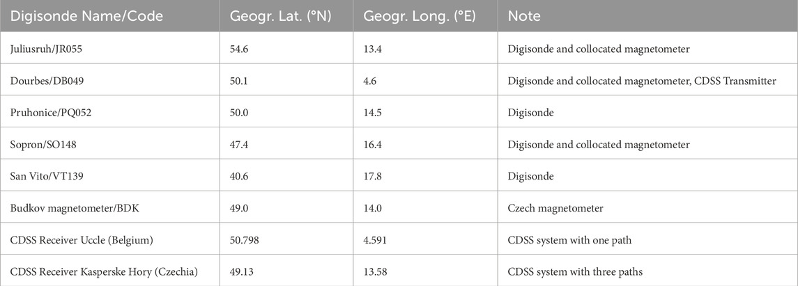
Table 1. Geographic location of Digisondes, Magnetometers, and CDSS receivers.

3 Results

3.1 Solar wind and geomagnetic activity

For the description of the forcing by the solar wind (SW) we use solar wind measurements by Wind spacecraft (Ogilvie et al., 1995) located at Lagrangian L1 point. After analyzing multiple parameters, for demonstration of solar wind geo-effectiveness during storm-time periods we provide the Bz, v, Np and epsilon parameters, i.e., the southward component of the interplanetary magnetic field (IMF) in the Geocentric Solar Ecliptic (GSE) plane, total solar wind velocity and proton density, and the Akasofu Epsilon, here in the form providing total energy input into the magnetosphere (Akasofu, 1981). For the two storms in the following plots we show that not having such correction of Epsilon considered could be misleading for the comparison of geoeffectiveness of the solar wind forcing. For geomagnetic description we used Kp index and Dst index. For a better orientation In Figure 1 and the following figures we also plot the time of the Sudden Storm Commencement (SSC) obtained from https://www.obsebre.es/en/variations/rapid, which indicate the start of the geomagnetic disturbance. Starting at the SSC time a short period (1–2 h) of a so-called initial phase is present until the Sudden Onset time, however this characteristic is difficult to identify precisely. The main phase of the geomagnetic storm starts from the Sudden Onset time until the time of the minimum Dstmin, which follows right after that with the recovery phase of the geomagnetic storm (see for more Tsurutani, 2000). We also add the time of minimum value of Dst to the figures.

3.1.1 March 2023 storm

Upstream solar wind parameters from Lagrangian L1 point show that ionospheric forcing by the fast solar wind (corotating interaction region - CIR) was significant already from March 21st. Geomagnetically March 22nd was a quiet day. The arrival of the interplanetary shock (interplanetary coronal mass ejections - ICME) front at 13:40 UT on March 23rd with gradually rising magnetospheric coupling became very geo-effective from 16:40 UT due to the start of prolonged significantly Bz negative interplanetary magnetic field continuing to the following day. As a result, a minor G1 geomagnetic storm (23 March) occurred.

The geomagnetic disturbance started with an SSC at 14:11 UT on 23 March (dashed red lines in left panels of Figure 1). The geomagnetic storm’s main phase lasted until the time of the minimum Dstmin that happened at 03:00 UT on March 24th with −163 nT (dashed blue lines in left panels of Figure 1) followed by a recovery phase of the storm (Figure 1).

3.1.2 April 2023 storm

Although there was negligible forcing by weak ICME till 20th April, and slightly disturbed period occurring from noon till midnight of 21st April, the period before the storm was characterized by generally slow solar wind. First significant impulse from ICME arrived with the interplanetary shock shortly before 17UT on 23rd April with the subsequent days of fast solar wind-shocked stream interaction region (SIR). ICME geo-effectiveness nevertheless diminished already on 23rd April around 22UT due to the IMF turning northward. This pre-energized the magnetosphere for the sudden impulse when the strong IMF (∼40nT, withstanding almost till the noontime) of the fast solar wind turned almost completely southward at 01UT on 24th April, only gradually turning back therefore being highly geo-efficient mainly till 9UT. It was observed as a moderate (G2) to strong (G3) geomagnetic storm. The geomagnetic disturbance started with an SSC at 17:35 UT (dashed red lines in right panels of Figure 1). The geomagnetic storm’s main phase lasted until the time of the Dstmin that happened at 05:00 UT on April 24th with −209 nT (dashed blue lines in right panels in Figure 1) and was followed by the recovery phase of the storm. Although the geoeffectiveness of the April storm (shown by Epsilon parameter) is higher than for the March storm, we remind here the necessity to consider the previous CIR/fast solar wind forcing which has resulted of considerably significant ionospheric effect of the first day of March storm compared to the start of April storm.

3.2 Digisonde measurement

3.2.1 Digisonde characteristics: March 2023

In Figure 2 we show critical frequencies foF2 and foF1 for stations JR055, DB049, PQ052, SO148, VT139 for the period 22 to 28 March 2023. Interesting feature in the F2 region is the increase in foF2 at noon on 23 March, before the SSC (14:11 UT). Relative increase is about 15%–20% for JR055, DB049, SO148 and PQ052 compared to median values (and about 25% and 13% compared to March 22nd), and about 10% for VT139. Analyzing the shape of the reflections in raw ionograms, during daytime on March 23rd no significant changes in the shape of the traces were observed.

Figure 2

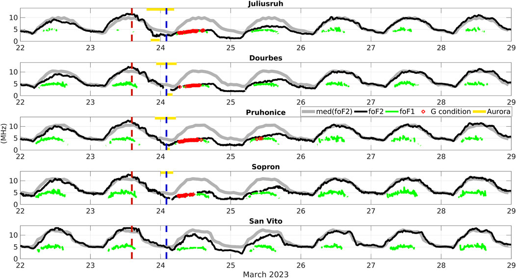
Figure 2. Course of critical frequencies foF2 and foF1 during March storm. Median values of foF2 are given in light gray. G-condition is denoted as red circles. Intervals with presence of auroral reflections are shown as horizontal yellow lines (upper for auroral F and bottom for auroral E). Vertical red and blue dashed lines denote SSC and minimum Dst, respectively.

Using the data with 5 min resolution shown in Figure 2 we see that on March 24th rapid decrease in foF2 is shown by more than ∼50% at JR055, DB049, PQ052 and SO148, and 15%–25% at VT139, respectively, compared to median values with progressive increase on the following day March 25th. The situation is complicated by the presence of G-condition when the foF2 values could not be estimated (discussed in following parts of the paper). On 26 March and following days the foF2 returned to the median values. Even more significant change was the decrease in night foF2 values. At JR055 station at 20:38 UT on March 23rd, and 3 hours later, at 23:53-23:58 UT the foF2 values at JR055, DB049, PQ052 and SO148 started to rapidly drop to about 50% compared to medians (∼2 MHz compared to ∼4 MHz). The decrease in night foF2 was even more pronounced in JR055 (∼1.3 MHz) on 24/25 March whereas at the other stations the night minima resembled 22/23 March values. Generally, the night decrease of foF2 was stronger in the northern located station Juliusruh compared to other stations.

During manual scaling of 23rd March ionograms we observed temporarily limited wave-like oscillation with ∼1.5 h period demonstrated as a shift in the foF2 towards lower frequencies and back (the limits of the frequencies are denoted by vertical lines and corresponding times in UT). The times and changes in foF2 parameters are given in Table 2 and the ionograms at the time of the start of oscillations at PQ052 and JR055 are shown in Figure 2.

Table 2

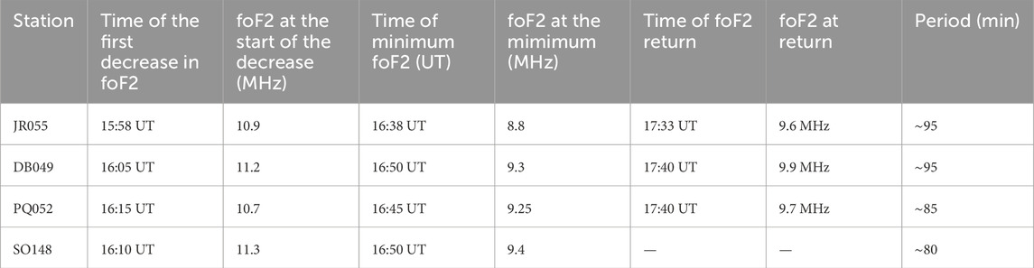
Table 2. Times and values of foF2 during the first oscillation on 23 March 2023.

For example, at JR055 the decrease started 15:58 UT with foF2 10.7 MHz. Local minimum was at 16:38 UT with foF2 8.8 MHz when the rise started again and foF2 reached 8.8 MHz at 17:33 UT. Approximate period of the oscillation (time difference between the end and start of the oscillation) are given in the right column. Values for DB049, PQ052, and SO148 are also given in Table 2. The oscillation at SO148 was weaker compared to other stations and we did not observe the increase in foF2 after 16:50. We did not observe the periodic change in foF2 at VT148. In Figure 3A, B) we show ionograms at the start of the oscillations and foF2 minima and returning values for PQ052 and JR055. A weaker manifestation with similar periodicity was observed at SO148 (starting at 16:10). This was a first (moderate) ionospheric response to changes in local geomagnetic field and a direct consequence of shock in solar wind observed at 13:30 UT in the L1 point. The estimated periodicity ∼80–∼95 min (Figure 3A, B; Table 2) was confirmed by wavelet decomposition (Figure 4). For the wavelet analysis, due to the occasional unavailability of foF2 during the G-condition starting on 24th March we used the highest critical frequency max (foF1, foF2) which was measured at the given time (i.e., foF1 during the G-condition) but this did not influence the results we present for the 23rd March. The increase in wavelet content was localized to approximately 16:00 (JR055) and 16:15 (PQ052) on 23rd March with a central period around 70–80 min (panels A, B in Figure 4). At the same time, a rather wide band of increased power content with a period of ∼2 h–3 h was present in the data (dashed white rectangles). We also detected an increase in wavelet content with the period of ∼6 h starting in the morning of March 23rd and lasting a whole day (Figure 4, panels A, B, the wavelet content ∼6 h is emphasized by dashed white rectangles). The increase in ∼6 h period we attribute to the very slowly decreasing solar wind Bz (Figure 1, panel A).

Figure 3

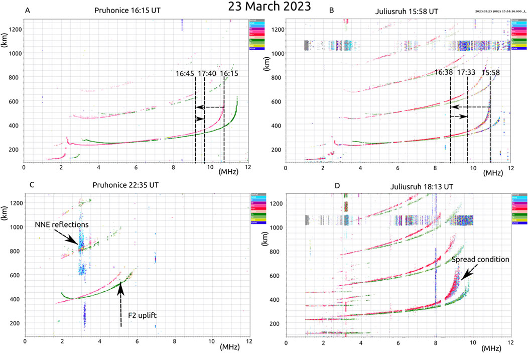
Figure 3. Example of ionograms on 23 March 2023 from PQ052 (left) and JR055 (right). The horizontal axis shows plasma frequency (MHz), the vertical axis shows virtual height (km). Sudden quasi-periodic oscillation in electron density (A)- PQ052, (B) JR055). Vertical dashed lines denote start of the foF2 decrease, minimum and following maximum of foF2, according to the arrows. The time above the lines is in UT. Note the undisturbed shape of ionogram traces. Start of the most significant changes is shown for PQ052 (C) and JR055 (D). At a given time the ionograms at both stations are followed by a rapid change in shapes of the traces and in electron density profiles.

Figure 4

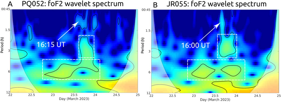
Figure 4. Wavelet spectra of foF2 from JR055 (A) and PQ052 (B). The arrows show short periodic change in foF2 corresponding to the first ionospheric response to the storm. Wave activity with periods between 2 and 3 h is denoted by upper white dashed rectangles. Persistent periodicity of about 6 h is denoted by bottom white dashed rectangles and is present for a whole day (PQ052) or for a most of the day 23rd March (JR055).

The most significant changes seen in the ionograms started first at 18:13 in JR055 as a sharp decrease in foF2 and development of spread conditions present in the ionograms which are a sign of non-planarity of the ionosphere (Figure 3, panel D). Decrease in foF2 and other significant ionospheric response was observed at the other stations about 50–60 min later than at JR055 (e.g., 19:00 PQ052). The decrease corresponds well to increased geomagnetic activity at collocated or near stations. The rapid decrease of electron concentration in the F2 region at most of the stations around 19:00 and strong uplift of the F2 region after 22:30 (e.g., at PQ052 at 22:35, Figure 3, panel C) are connected to the large peak of local geomagnetic activity at 19:00 and a later peak around 22:30 UT. We also observed auroral reflections in the F as well as E regions (these periods are denoted by yellow stripes at the top for F region or at the bottom of the panels for the E region auroras). The occurrence of auroral reflections up to the 05:15 of March 24th also corresponds to the most serious disturbance in geomagnetic activity which lasts up to about 05:30 UT.

Electron concentration in the F1 region was also significantly depleted. Critical frequencies foF1 dropped from maximum noon values 6 MHz (VT139), or 5.5 MHz (all other stations) on days before the storm to 4.7 MHz (VT139, 22% decrease) and 4.5 MHz (all other stations, 18% decrease) on March 24th compared to quiet time. The foF1 parameter was decreased also on March 25th with noon values 5.5 MHz (VT139) and 5 MHz (all other stations) and returned to normal values on 26 March. We did not observe significant changes in minimum frequency fmin during the March storm.

Statistical analysis of the data represented as boxplots for each particular day using foF2 and foF1 parameters is shown in Supplementary Material 1: Boxplots foF2 and foF1, left panels. This type of visualization (detailed explanation is in the text in the Supplementary Material 1) gives us a recapitulatory overview of the foF2 and foF1 changes. The above described features from Figure 2 as pre-storm enhancement on 23 March as well as the decrease in foF2 after the SSC are observed. Decrease of median daily values on 24 March and slow return to quiet-time conditions on 25 March at all stations (weaker but noticeable at VT139) agree with the description using Figure 2. The decrease in foF1 on the day following the SSC (i.e., on 24 March) is well seen in the boxplots for data from all stations. While the foF1 medians on 25 March was still slightly below the medians observed on the following days at JR055, DB049, SO148, and VT139, it seems that the foF1 parameter at PQ052 already returned to normal values on 25 March. Interesting feature is a low variance in foF1 for both 24 and 25 March at the Dourbes station, compared to all other stations (especially VT139).

3.2.2 Digisonde characteristics: April 2023

In Figure 5 we show critical frequencies foF2 and foF1 for stations JR055, DB049, PQ052, SO148, VT139 during the April storm. The most significant observations are following: A drop in foF2 is observed at 13:40 UT at all stations on 23 March, i.e., ∼4 h before the SSC (17:35 UT), with no apparent connection to significant changes in the solar wind. The most dramatic changes were observed on the ionograms started at JR055 (19:08), DB049 (19:35), PQ052 (19:55), SO148 (20:05) demonstrated as sudden appearance of very well developed spread condition in F2 layers and fast decrease in electron concentration in the F2 region. The times correspond well with the increased geomagnetic activity from the collocated magnetometers (e.g., sharp oscillations of horizontal component of the magnetic field H starting at 19:30 UT at DB049 and PQ052) and follow the first SW shock measured at 17:10 UT in the L1 point. Significant decrease by ∼3 MHz (about ∼60% decrease) compared to median values during night hours 23/24 and 24/25 April was the most significant deviation from previous state by means of foF2. The night values approached a quiet situation on the night of 25/26 April. Decrease in morning and noon values of foF2 on 24 and April 25th by ∼40% was observed at all stations while the foF2 nearly agreed with medians in the afternoon and night during both days of April 24th and 25th. Similarly to the March event, the situation on April 24th and 25th was complicated by the presence of G-condition. The situation slowly returned to quiet state on 26 and 27 March, however with the exception of VT139, the foF2 characteristics were still below medians.

Figure 5

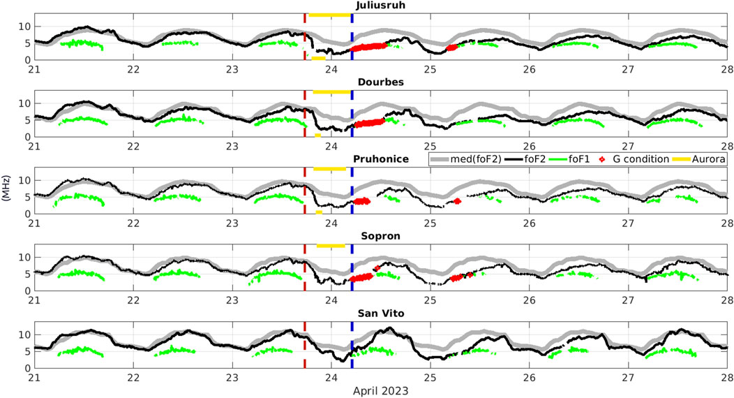
Figure 5. Critical frequencies foF2 and foF1 from April storm. Median values of foF2 are given in light gray. G-condition is denoted as red circles. Intervals with presence of auroral reflections are shown as horizontal yellow lines (upper for auroral F and bottom for auroral E). Vertical red and blue dashed lines denote SSC and minimum Dst, respectively.

The relative decrease in foF1 was observed on April 24th around ∼8% compared to the quiet situation at JR055, DB049, PQ052, SO148 with a slow return to quiet time values from 25 to 27 April. The change in foF1 was not observed at the VT139 station. We did not observe significant changes in minimum frequency f_min during the studied period.

The statistical analysis using the boxplot visualization (see Supplementary Material 1: Boxplots foF2 and foF1, right panels) brings following main results: The decrease in foF2 was observed at all stations on the day of SSC on 23 April as well as on 24 April, however at all stations the interpretation of the decrease was complicated by a decline in foF2 during previous days starting on 21 April. Therefore we show the plots starting 1 day earlier compared to the March boxplots already from 21 April. The most significant decrease in foF1 after the SSC was observed at JR055, however the decrease was seen at all stations. Comparison with the March event shows that the decrease in foF1 during the April event was less significant but it was observed at all stations with a decreasing trend towards southern located stations (the highest relative change in foF1 was observed at JR055, the smallest changes was observed at VT139).

3.3 G-condition and auroral activity during the March and April event

The ionograms’ quality can be significantly affected by an intriguing phenomenon known as G-condition. In instances where the E and F1 regions of the ionosphere are well developed and easily detectable, an anomaly arises when the critical frequency of the upper F2 region falls below foF1. This situation makes the F2 region inaccessible to Digisonde measurements, effectively rendering it “invisible” (refer to Figure 6). Notably, during both events under study, the ionospheric response was marked by prolonged periods of the G-condition, as depicted in Figures 3, 5. Both events exhibited similar characteristics across all observation stations, with the exception of VT139. The G-condition was observed during morning and around noon hours, but completely absent in the afternoon.

Figure 6

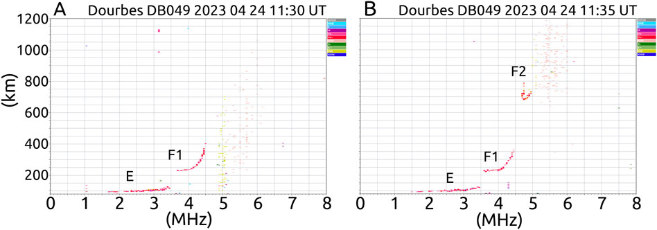
Figure 6. (A) shows an ionogram with visible E and F1 layers and missing F2 layer (G-condition) on April 24th (11:30 UT). (B) shows an ionogram 5 minutes later with E, F1 and F2 layers. The situation in the E and F1 regions is similar in both ionograms.

During the event in March, the occurrence of the G-condition on March 23 was as follows: 66% at JR055, 48% at DB049, 61% at PQ052, 50% at SO148, and 0% at VT139. Following day, March 24, G-condition was observed only for a very short time interval (2.4% occurrence) at PQ052 and did not occur at the other stations. The percentage is computed as the ratio between ionograms exhibiting the G-condition on a given day and all ionograms at which the F1 layer was observed (Figure 2). During the April event, the percentage of G-condition presence on April 24 was 60% at JR055, 50% at DB049, 32% at PQ052, 35% at SO148, and 0% at VT139, and 14% at JR055, 0% at DB049, 5% at PQ052, 9% at SO148, and 6% at VT139 on the 25th of April 2023 (Figure 5).

In the ionogram mode the Digisonde allows the detection of not only vertical (normally+/-15 deg off zenith) but also oblique reflections in six azimuthal sectors of 60 deg width. Thanks to the specific orientation of the receiving antenna field comprising four cross-loop antennas the Digisonde clearly distinguishes direction and polarization of the arriving echo. During both March and April events we observed auroral activity by means of Digisonde (Figures 2, 5 - periods of Aurora are denoted as yellow lines) as well as optical measurement (Figure 7) demonstrating auroral oval expansion. In Figure 7 we see a complementary observation of an Aurora by means of an optical camera aimed toward the north together with ionograms showing oblique reflections in a northward (N) direction. Except for VT139, at all four stations using the Digisondes we observed oblique reflections from the NNE and NNW direction (due to the configuration of the receiving antenna field there is no possibility to measure “pure” N direction) from the F2 region, and from the E region at JR055, DB049, PQ052. The periods of auroral occurrence observed by Digisondes are denoted as yellow horizontal lines on top (F2 region auroras) or bottom (E region auroras) of individual panels in Figures 2, 5. The occurrence of auroral reflections is clearly dependent on the position of the stations. During March 2023, the auroral observations started at the JR055 station as the first occurrence of such oblique reflection was recorded at 19:13 UT, and about 3–4 h later at the stations located further from the auroral oval DB049, PQ052, SO148. The end of the oblique F2 reflections occurred at a similar time at all four stations. The F2 region aurora was observed for longer periods of time compared to the E region aurora, it started earlier and also finished later. Presence of blanqueting sporadic layers after 23:43 UT on 23rd March at JR055 complicates exact estimation of auroral E presence and comparison with PQ052 and DB049.

Figure 7

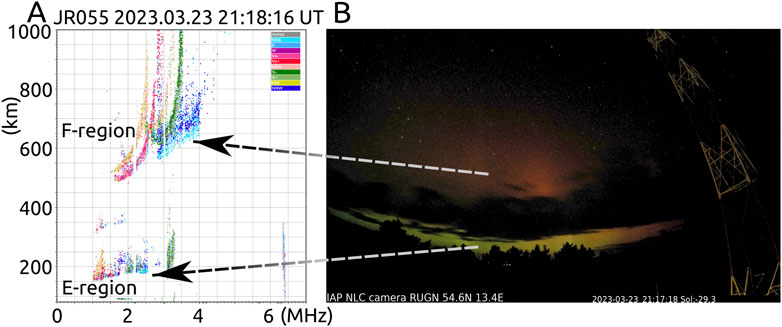
Figure 7. Simultaneous digisonde observation of oblique reflection at JR055 on March 23, 21:18:16 UT panel (A). Dark and light blue denote NNW and NNE direction of reflections, respectively, red and green reflections are vertical O and X-modes. Optical observation of well developed Aurora Borealis is seen in panel (B). The camera is aimed towards the north on March 23, 21:17:18 UT. Aurora is observed in both regions E (green Aurora, ∼20 deg elevation) and F (red Aurora, ∼40–45 deg elevation).

3.4 Shape of the electron density profile, parameter B0, and TEC

Figures 8, 9 show variations in the B0 parameter during the March 2023 and April 2023 events. Little changes were registered during the beginning of the storm in the evening on March 23rd. The most significant changes occur during 2 days and are highlighted by the dashed rectangles. The sharp rise in B0 is observed from morning hours on March 24th at JR055, DB049, and PQ052 station but the data are intermittent due to presence of G-condition when the electron density profile could not be estimated (Figure 8). Noticeably increased is the B0 parameter also in SO148 but contrary to JR055 and DB049 stations where we still obtained ionograms allowing for the electron density profile estimation, the information from the period of the (probable) B0 maximum at SO148 is completely missing. Slight increase in VT139 is also reported. Increase in B0 was observed even the following day, during low to moderate geomagnetic activity, as shown in the upper panels of Figure 8. Despite the described limitation in B0 estimation, the increase in B0 on March 24th and 25th was remarkable. It reached up to 233%, 56% (JR055); 537%, 77% (DB049); 300%, 156% (PQ052); 133%, 200% (SO148); and 70%, 55% (VT139), with both values representing an increase during maxima on 24th and 25th March compared to the days before the storm.

Figure 8

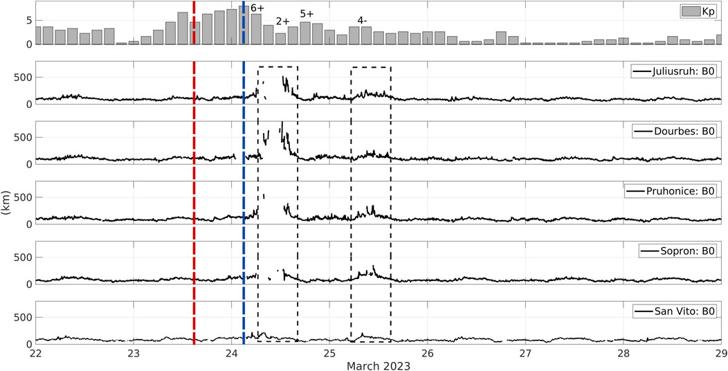
Figure 8. B0 parameter at ionospheric stations during the March event. Upper panel shows the geomagnetic Kp index for comparison. Dashed rectangle denotes periods of increased B0 values. Vertical red and blue dashed lines denote SSC and minimum Dst, respectively.

Figure 9

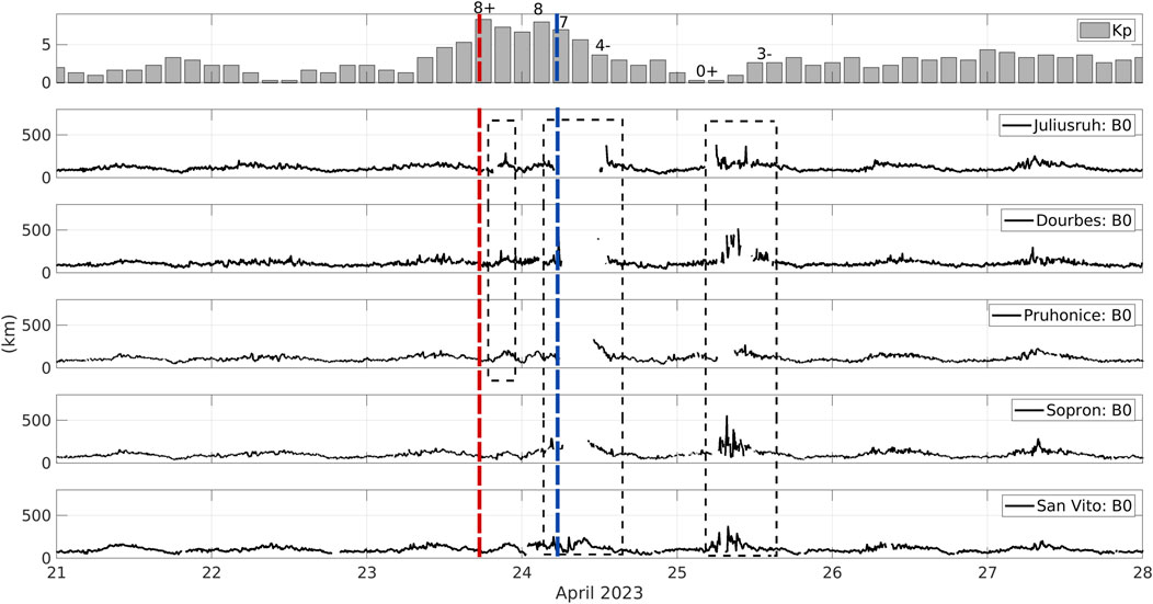
Figure 9. B0 parameter at ionospheric stations during the April event. Upper panel shows the geomagnetic Kp index for comparison. Dashed rectangle denotes periods of increased B0 values. Vertical red and blue dashed lines denote SSC and minimum Dst, respectively.

In contrast to the March event, the B0 changes during the April event occurred already during the evening and night just after the start of the storm on April 23rd, most notably at JR055, PQ052, SO148 (left dashed rectangle in Figure 9). The changes were followed by a less severe relative increase compared to the March event on April 24th and comparable changes on the following day (we compare first and second day in each event). The changes in B0 on April 24th and 25th reached up to 126%, 128% (JR055); 111%, 157% (DB049); 60%, 30% (PQ052); 64%, 240% (SO148); and 40%, 125% (VT139) compared to the days before the storm. Relatively low increase in Pruhonice on April 25th may be influenced by missing data due to the short-time presence of G-condition leading to a missing B0 maximum.

In the plots incorporated in Supplementary Material 2: Northern Hemisphere TEC Polar Maps for 23 March 2023 we show temporal progress of TEC in the northern polar region. In plots shown in Supplementary Material 3A: TEC over Europe 22–24 March 2023 and 3B: TEC over Europe 22–24 April we show side-to-side comparison of TEC above the European sector for corresponding times of the day before storm, the day of the storm and the day after the storm.

3.5 DDM - Digisonde Drift Measurement results

In Figure 10 we show vertical speeds of ionospheric plasma using DDM. In the text we discuss drift measurements for the Pruhonice, Dourbes, and Juliusruh stations. The measurement was also conducted on SO148 station but the quality of results at this station does not allow for proper interpretation. Drift measurements in Pruhonice and Dourbes were conducted for the F layer in autodrift mode with a 5-min cadence. For the Juliusruh station, the possibilities of drift evaluation are relatively limited because measurements were only taken during nighttime hours, between 18 UT and 6:30 UT, with a 15-min cadence.

Figure 10

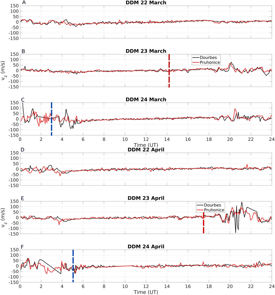
Figure 10. Vertical speeds of ionospheric plasma from DDM at Dourbes and Pruhonice stations during March event panels (A–C) and April event panels (D–F). Vertical red and blue dashed lines denote SSC and minimum Dst, respectively.

During the March 2023 event in Pruhonice and Dourbes, the vertical velocity measured on 22 March 2023, and March 23, until about 18:30, fully corresponds to the behavior observed under quiet conditions. Negative peak during dawn, followed by a gradual increase from negative values, crossing zero around noon, and then turning positive before the onset of the negative dusk peak (Figure 10, panel A). The magnitude of the horizontal component of the drift velocity rarely exceeds 100 m/s. The first signs of the storm are reflected in the drift measurements at the Pruhonice station at 18:33 UT (Figure 10, panel B), showing a significant decrease in the vertical component.This initial impulse shows a milder descent in the Dourbes measurements. At all the three stations, during the night from March 23 to March 24, episodes of significant oscillations in vertical drift are evident. Detected values exceed 100 m/s. Clearly defined skymaps with extreme horizontal velocity values appear both in Pruhonice and Juliusruh (see Supplementary Material 4: Skymap as an example of well defined SKY map from JR055 during the intense ionospheric disturbance). In Pruhonice, horizontal velocities often exceeded 350 m/s and sometimes even reached up to 700 m/s, with movements in the azimuthal range of 240–270° (towards SW-W). Clearly defined skymaps with large detected velocities also appeared in Juliusruh, with movements mainly in the azimuthal range of 270–290°, i.e., towards W.

On March 24, from 03 UT, drift activity substantially weakened and during daylight hours, it practically resembled calm behavior (Figure 10, panel C). In the evening of March 24, between 20:30 UT and 21:30 UT, brief but distinct oscillations were observed in the vertical component, with less pronounced horizontal components. In the following days, no clear indications of storms were prominent in the drift data.

Prior to the April storm, typical patterns under quiet conditions were observed again, as described above (Figure 10, panel D). The first signs of the April storm appeared in Pruhonice and Juliusruh around 19 UT on 23 April 2023. A rapid decline in the vertical component was observed, transitioning from +30 m/s to −50 m/s. In the subsequent hours, the vertical component oscillated between +150 and −150 m/s (Figure 10, panel E). As for horizontal velocity, in this case, very high-quality skymaps were recorded, allowing reliable determination of all velocity components. In Pruhonice, movements in azimuths between 170 and 290° (towards S and W) with speeds mostly up to 550 m/s were observed, but occasionally values of 800 m/s were recorded. For Juliusruh, the magnitude of the detected horizontal velocity reached up to 400 m/s, with azimuth mainly between 260 and 310°, i.e., towards W - NW. In the following days, no significant storm indications were observed on all three stations using DDM.

3.6 CDSS - Continuous Doppler Sounding System results

Upper panels A, B in Figure 11 show Doppler shifts for three different paths between the transmitting and receiving stations in Czechia. Intervals with missing data are caused by decrease of maximum plasma frequency below the sounding frequency of the instrument. Analysis of oscillation of the signal shows that the dominant periods during the March event are concentrated in the evening hours after ∼19 UT on March 23rd with periods about 40–90 min with the most significant period ∼70 min. During the following 2 days, only a short period of data was recorded between ∼15 UT and ∼18 UT on 24 March showing relatively low but still noticeable wave activity at periods ∼50–90 min and azimuth towards south, and morning to midnight data on 25 March with the most dominant oscillations after sunset, but much less significant compared to 23 March (panel C), with two main domains of periods around 4–7 min and around 70 min.

Figure 11

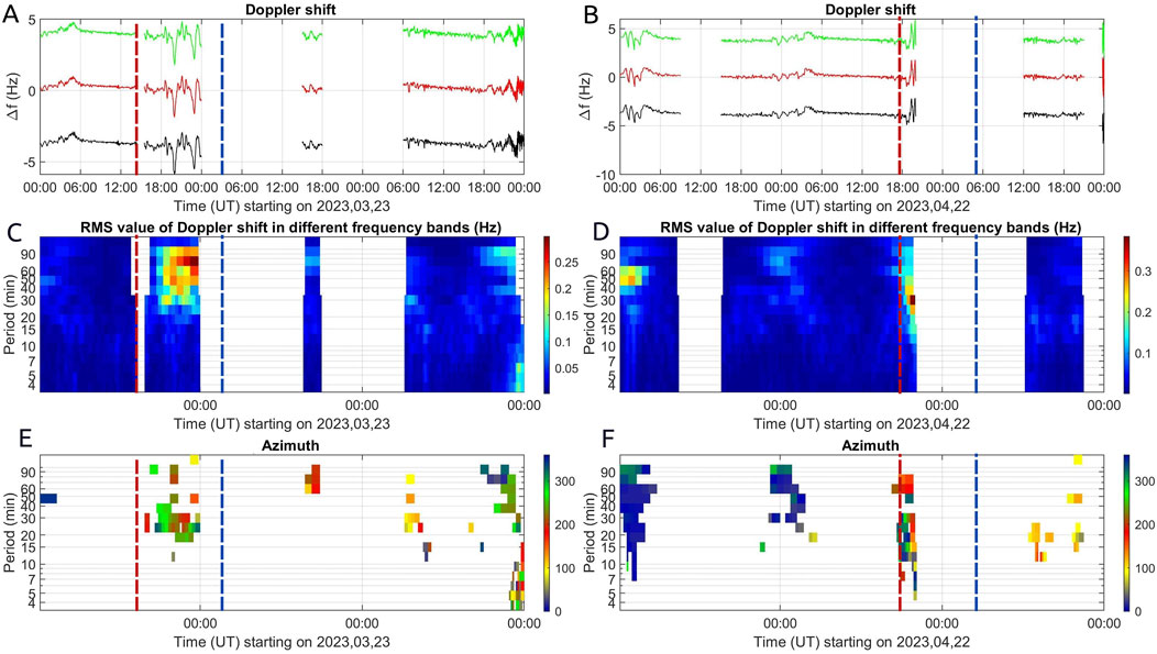
Figure 11. Doppler shift frequencies of spectral density maxima for individual transmitter-receiver pairs (including artificial frequency offsets 4 Hz) from March 23 to March 25 (A) and April 22 to April 24 recorded at 4.65 MHz (B). Dynamic spectra (periodograms) of Doppler shift signals for March and April (C, D) and the propagation azimuth of waves, displayed as function of period and time for March and April (E, F). Vertical red and blue dashed lines denote SSC and minimum Dst.

The rise of wave activity during the April event on April 23rd started about 19:00 UT with the central period about 30 min. The observation was possible until ∼20:15 UT when the sounding frequency exceeded the plasma frequency and the signal was not reflected back. Phase delay between the signals is used for computation of horizontal speeds and azimuths of disturbances shown in panels E, F of Figure 11. Increase in wave activity during the March event starts suddenly around 19 UT on March 23 (Figure 11, panels A, C, E), rapid changes occur at 20 UT and 23 UT with a direction mostly westward and southward. The direction shortly after the SSC on 23 April is predominantly towards the south and west.

Detailed CDSS spectrograms for the start of both storms are shown in panels A, B in Figure 12. Figure 12 shows a comparison of vertical speed of plasma vz from the F region using DDM and CDSS methods (left panels show March 23rd 18:00 to 20:15 UT, right panels show April 23rd 18:00 to 20:15 UT). The CDSS signal for Czechia was computed as a mean value of the four signals shown in panels A and B. Before the fast ionospheric changes, vz was close to zero. On March 23rd, the first observed increase in vz was between 18:45 and 19:00 UT. The second peak was observed after 19:45 UT reaching at both stations ∼70–90 m/s. These values were exceeded in the later phases of the storm as shown in the previous section, however only detected by DDM due to a decrease in maximum plasma frequency exceeding the sounding frequency of CDSS. On April 23rd, till ∼18:30 UT the vertical speeds at both stations were close to zero. After that, the first peak in vz reached ∼40 m/s between 18:30 and 19:00 and the second, more pronounced peaks reached −50 and +50 m/s speeds of vz. In both events, the vz was similar at DB049 and PQ052 but the record at DB049 was slightly delayed by about 3–5 min. We also compared the vertical speeds with local geomagnetic measurement. On March 23, the first peak corresponded well with the E-component of local magnetic field measured in Czechia but not in Belgium (E-component is a component of horizontal magnetic field perpendicular to magnetic south-north direction, only measured in Czechia). On March 23, the variations in the H-component were reflected in the vertical plasma drift in less obvious ways at DB049 and PQ052 station. On April 23, we also observed a good agreement between magnetic E−component and vz at PQ052. The rise in E between 18:30 and 19:00 UT on 23rd April corresponds to upward plasma movement and the oscillations between 19:15 and 20:15 UT have also the same period. Using the magnetic H component we observed that the magnetic variations were delayed by about 3–5 min at DB049 compared to PQ052.

Figure 12

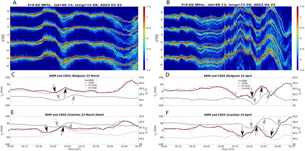
Figure 12. Vertical plasma drift vz at Dourbes and Pruhonice during March 23rd (left panels) and April 23rd (right panels). Panels (A, B) show four original CDSS traces from Czechia separated by 4 Hz. Panels (C–F) show excellent agreement of DDM (solid black) and CDSS (dashed red) derived vz values. Note the opposite signs of vz vs the Doppler shift Δf: Positive values in panels (A, B) denote positive Δf, therefore descend of the plasma, whereas positive values in panels C–F denote positive orientation of speeds, therefore upward moving plasma. Geomagnetic field is shown using H (horizontal component) for both stations and E component (only Czechia). Black and gray arrows denote corresponding/related variations in vz and H.

4 Discussion

In the paper we summarize data from various ground based ionospheric techniques and compare the extent of two ionospheric storms separated by 1 month. Both March and April 2023 storms are among the most severe ionospheric events in the SC 25 (although they were surpassed by the May 2024 superstorm). Although the solar forcing during both events is not identical (especially the epsilon parameter is nearly three times higher during April than during March storm) we observed rather comparable results at the European midlatitude stations, namely, vertical plasma drifts, auroral reflections and changes in the shape of electron density profile. The first, relatively moderate ionospheric response observed as oscillation with period ∼1 h occurring between 15:58 UT (JR055), 16:10 - 16:15 UT (SO148, PQ052) on 23rd March did not seem to have an evident or well defined source in solar wind parameters.

A significant finding of our study is the notable increase in electron density at the peak height of the F2 layer on March 23 at all stations except VT139 (Figure 2) where we did not observe similar distinct increase in foF2 but the increase was observed statistically (see Supplementary Material 1: Boxplots foF2 and foF1). The weak response at VT139 is in agreement with observations of Paul et al. (2024) who report no positive deviation (no positive storm) at the southernly located stations San Vito, Rome, Athens, Nicosia. The increase at northern located stations reached up to 20% compared to the previous day. According to Huang et al. (2005), among various explanations for such increases, the daytime short-duration surge in mid-latitudes, occurring a few hours after the sudden onset of a storm, emerges as a potential reason. In this scenario, large-scale gravity waves originating in the disturbed auroral zone propagate towards middle latitudes, causing an uplift of the F region along magnetic field lines and subsequently reducing recombination, leading to increased electron densities. A plausible explanation for the pre-storm increase even before the SSC could therefore be the gradual growth of solar wind density and total magnetic field.

We observed a decrease in both foF2 and foF1 parameters after the start of the two events, indicating a negative ionospheric storm (Figures 2, 5 and Supplementary Material 1: Boxplots foF2 and foF1). This decrease persisted for 2 days following the onset of the storm. The reduction in foF2 was particularly pronounced, both during daytime and nighttime, comparable to the strongest storms observed in previous solar cycles (e.g., Berényi et al., 2023). Consistent with expectations, the VT139 station, located further south in Italy, experienced less pronounced impact in the F2 region during the storms, but still noticeable in decrease of electron density in night and morning hours. As explained by Oyama et al. (2024) the large decrease of electron density in the F region was a result of upward transfer of molecular-rich air from lower altitudes and therefore affecting the production/loss ratio by substantial amplification of the dissociative recombination process.

Notably, there was a significant and deep decrease in electron concentration in the F1 region, affecting all stations for two consecutive days during the March event, with similar relative changes observed. During the April event, a relatively strong decrease in foF1 was observed at four ionospheric stations of total five, though less severe compared to the March storm, and only slightly affected the VT139 station. As the F1 region ionization is directly connected to the solar ionization which did not change significantly, the decrease in plasma frequency is a result of plasma outflow from the F1 region. Spread conditions were evident in the ionograms during both events (Figure 3), characterized by diffused reflections instead of well-defined echoes. These diffused reflections indicate a change from the typical plane mirror-like reflection of the quiet ionosphere, resulting in multiple reflections from the disturbed ionosphere.

The wavelet analysis was performed during both events for the highest F region critical frequency (Figure 4). During the March event, periodicity in the 6 h domain observed in foF2 since morning March 23rd was probably connected to the very slow changes in SW characteristics, namely, decrease in SW Bz and rise in B and SW density between 03 and 06 UT (it is difficult to estimate exact start of SW forcing). Except for this, the most significant observation is well defined ∼60–90 min periodicity around 16 UT in foF2 clearly identified to changes on ionograms as well as ∼3 h periodicity in the same time. The foF2 response is not seen in the wavelet spectrum after the start of the major phase of the storm after 19 UT on March 23rd. Although surprising, it can be explained that the possible fast oscillations in foF2 were not detected using wavelet analysis because the Digisonde measurement has 5 min time resolution.

The results from CDSS spectral analysis (Figure 11) show that the oscillations present between 18:30 and 00:00 UT on March 23rd are in the range of 20–90 min with a central period about 70 min. The most dominant periodicity during the initial phase of the April storm on April 23rd (∼19:00 - 20:30 UT) is in the range 15–60 min with a well defined central period 30 min. The CDSS spectral analysis is limited due to occasionally missing data but allows for very well defined temporal resolution of the wave processes not obtainable by means of DDM method.

4.1 Electron density distribution and shape of the electron density profile

Both events were characterized by the presence of G-conditions (Figures 2, 5) at JR055, DB049, PQ052, and SO148 stations (not at VT139, although during April 25th the foF2 and foF1 values were very close). The respective percentage of G-condition occurrences in both events roughly increased towards the geographic north, with approximately 66% (March) and 60% (April) of G-condition occurrences at JR055, and about 50%–60% on March 24th and 32%–50% on April 24th. It is worth noting that the statistics may be slightly biased due to occasional complete blanketing caused by Es and other issues such as low quality of ionograms, but it still provides a very good general idea about the distribution of this phenomenon. The tendency of lower latitudes to have a lower percentage of G-condition presence is in agreement with the general effect of foF2 decrease related to geographic position. Ionograms showing G-condition situations were typically observed for several hours consecutively; however, these periods were sometimes interrupted by ionograms with a visible F2 layer and foF2 just slightly above the foF1, typically with up to a 0.5 MHz difference. Although information about the situation in the F2 region is lacking, it can be assumed that the foF2 did not fall significantly below foF1 for most of the time and was probably only several tenths of a MHz below foF1 and accidently increasing slightly above foF1 for a short period of time. However, we propose statistical estimation of foF2 during G-condition as an open question and interesting topic for future studies using further analyses. Important result is observation of G-condition during periods of moderate geomagnetic activity, e.g., Kp ∼4 on March 25th at PQ052 or during relatively low Kp < 3 at JR055, PQ052, and SO148 on April 25th. Our observation complements the statistical study of Deminov et al. (2011) who showed that the probability of G-condition increases with an increasing geomagnetic activity and exponentially depends on the Kp index. Therefore, more complex processes involving the neutral atmosphere play an important role in this phenomenon.

The observation of G-condition only during morning and around noon hours (not at all in the afternoon) aligns with the findings of Lobzin and Pavlov (2022), who demonstrate that G-condition is more likely to occur during the first half of the day than during the second half at middle and high latitude regions. This is also in agreement with a paper of Gordiyenko (2023) who analyzed a long-lasting negative disturbance during the major space weather event at five Middle Asian ionospheric stations.

Our findings can also contribute to the improvement of ionospheric modeling, as the most commonly used inversion models for electron density profile computation are based on the information of the main ionospheric parameters such as foF2 or the entire or substantial part of the ionogram (e.g., F2 layer, Huang and Reinisch, 1996; Titheridge, 1995; Šauli et al., 2007 among others). We focused on analyzing the shape of the electron density profile using parameters B0 (Figures 8, 9) and B1. The estimation was complicated by the occurrence of G-condition, during which the shape of the electron density profile in the F2 region could not be computed due to missing data (as mentioned earlier, this situation occurred up to 60% of the daytime period when the F1 region was present). Consequently, we may have missed capturing the most extreme values of B0 and B1. The largest increase in B0 (was observed in JR055 on March 24th (Figure 8, more than 230% increase compared to quiet time) with gradually less increased but still significantly impacted parameters at DB049, PQ052, SO148, VT139 (∼70% increase). Interestingly, a high increase in B0 was observed during periods with moderate geomagnetic activity on March 25th and even very low geomagnetic activity on April 25th (Figure 9).

Although the increases in B0 are only informative as they originate solely from ionograms with a developed F2 layer (and therefore the extreme values may be missed in the statistics), it is evident that not only the electron density in both the F2 and F1 regions was heavily affected but also the shape of the electron density profile was strongly modified. An important finding is that the changes in the shape of the electron density profile, as indicated by B0, were observed at all stations, including the southernmost located VT139, where the F2 electron density was only very slightly affected. Much less significant changes in B1 parameter were observed and no convincing results regarding the proportion of changes/variation in B1 attributed to storm activity compared to other reasons can be given. This finding is in agreement with the finding of Verhulst and Stankov (2023), who demonstrated much less sensitivity of B1 during disturbed ionospheric conditions compared to B0.

4.2 Auroras and plasma dynamics

Both March and April events were accompanied by a presence of auroral reflections (Figures 2, 5) as well as optical observations of Auroras (Figure 7). The auroral reflections are typically observed in auroral regions but are much less ubiquitous at midlatitude stations as DB049, PQ052, or SO148. The relatively long periods of auroral activity and their spatial extent reaching as low as ∼ 47°N in both March and April events, as well as repeated observation of midlatitude auroras in September and November 2023 February 2024 and most significantly in May 2024 confirm relatively high frequency in disturbances of the Earth’s magnetic field influencing the ionosphere and it is a result of the approaching solar maximum of SC 25. It also shows that solar activity seems to be comparable to the previous strong solar cycles in modern maximum (e.g., SC 22) and confirms not only the rise of the solar activity but also the increase in severity of ionospheric disturbances in current SC 25.

Using multi-instrumental analysis, we are able to describe ionospheric dynamics in the F2 region in detail. Both events show excellent agreement between DDM (Figure 10) and CDS (Figure 11) computed vertical speeds in Belgium and Czechia. The agreement between the data during both disturbed periods is very high (Figure 12) and confirms that both methods are good tools to describe the vertical plasma dynamics. Results from both Belgium and Czechia show negligible phase shift between signals at different sites located approximately 700 km apart.

According to both DDM and CDSS, increased wave activity starts at 18:30 UT on March 23rd in Czechia and Belgium in agreement with rapid changes observed in the ionogram data. The oscillations in Czechia are aligned with the E-component of locally measured geomagnetic activity and at both Belgium and Czech stations correlate with the H-component of local geomagnetic field (Figure 12 - panel C, E).

During the April event, slightly positive (upward) plasma motion sharply changes direction on 23 April at 19 UT, reaching up to −50 m/s in the following ∼20 min and consequently oscillating with the same values at both stations. Comparison of local horizontal vector H and the peak in upward speed of plasma at both stations DB049 and PQ052 shows that both the geomagnetic and ionospheric changes in the later phase occur about 5 min later at DB049 than at PQ052 station on April 23rd. The changes in the horizontal vector of geomagnetic activity H correspond with the initial phase, but later both vz and H seem to have no simple correlation. The used magnetic E-component corresponds well with the vertical plasma motion.

We also analyzed the horizontal components of the plasma drifts. During the March event, the horizontal direction towards the west and southwest after 19 UT on March 23rd, estimated by CDSS using phase shift between individual paths in Czechia, perfectly agrees with DDM results (also showing west and southwest direction of plasma). During April, westward and northwestward direction of plasma at JR055 station and southward and westward directions at PQ052 station were observed. During this event, the results from CDSS show south and south eastward propagation.

From previous studies like Heilig et al. (2022) it is stated that the MIT minima (which is the ionospheric footprint of the plasmapause) is accompanied with a strong horizontal westward plasma motion with around 500 m/s. Poleward wind surges during the night, reaching approximately 100 m/s, are primarily due to the poleward Coriolis effect arising from significant westward wind amplitudes (see Zhang et al., 2015; Tulasi et al., 2016; Huang et al., 2018; Berényi et al., 2023). During our storm cases the CDSS and DDM results are in good agreement with the conclusions of previous studies. On March 23rd after 19 UT over Czechia most probably the MIT minima caused the CDSS and DDM detected west and southwestward plasma motion when the speed reached up to 700 m/s. During the April storm event on April 23rd after 19 UT at JR055 the plasma drift velocity reached up to 400 m/s toward W-NW, at the same time at PQ052 was mostly 550 m/s but occasionally went up to 800 m/s and the motion was south and westward. This suggests that the MIT minima was over PQ052 when the speed reached the highest value. The equatorward motion of the MIT, thus the shrinking of the plasmasphere during the main phase of the geomagnetic storm, is also confirmed by the auroral reflection also observed at the midlatitude stations (PQ052 and SO148). Our present results agree with Paul et al. (2024), who concluded that the MIT reached 55° on 23 March based on the electron density profiles measured by the Swarm satellite data.

Both limitations and benefits of CDSS and DDM methods exist. Firstly, using DDM at SO148 station did not show significant vertical changes at the station during neither the March or April events. Manual analysis of the ionograms also revealed that the sensitivity of the SO148 instrument compared to JR055, DB049, and PQ052 instruments was noticeably lower (for further information about the differences in DPS-4D sensitivities see chapter 3.2.2 in Szárnya et al., 2024).

Generally, the DDM method can provide us with very accurate estimations of vertical as well as horizontal components, the latter especially during disturbed situations when the ionosphere allows a high number of reflection points. Downfall of CDSS is that it fails in situations when the sounding frequency is above the highest plasma frequency in the ionosphere, typically during the night, but also during disturbed and therefore interesting periods with decreased foF2. The doubtless benefit of CDSS is its high temporal resolution. Unlike DDM, the multi-point CDSS does not measure the horizontal plasma drifts but rather horizontal propagation of TIDs. The analysis of vertical plasma drifts using both CDSS and DDM confirms their credibility due to close quantitative results. Important advantage is also that both methods are completely independent. We assume that a) the similar vertical movement of ionospheric plasma at different ionospheric stations and b) the very good agreement between geomagnetic field changes and vertical plasma speeds in studied areas suggests the ExB drift as the most probable cause of the vertical plasma movement.

Our findings are in qualitative agreement with observations of Li and Jin (2024) in April 2023 in the Asian sector. They reported TIDs of 760–1,300 m/s from high latitude region to low latitude region with a period of about 40 min generated by periodic energy input from the auroral area, and also poleward TIDs with a velocity of approximately 600–750 m/s and similar period. Liu et al. (2019) reported TIDs related to the 2015 St. Patrick’s Day geomagnetic storm with the propagation direction almost slightly southwest and southeast in the western and eastern sides of this region. Reported period, trough velocity (vt), crest velocity (vc), and wavelength of the LSTIDs in the sector are approximately 75 min, 578 m/s, 617 m/s, and 2,691 km, respectively. Panasenko et al. (2023) reported LSTIDs originating during enhancement in auroral activity. from the ionosonde data. The magnetic storm-related LSTIDs exhibit equatorward propagation with the horizontal phase velocities of 546 m/s and 576 m/s, with dominant periods of 135–150 min and 165–180 min. According to Kishore and Kumar (2023) the observed wave activity evolves during the storm time. They show differences in TID propagation characteristics for March and June 2010 storms in the Australian region. The propagation directions were equatorward with east/west deviations. Lower period (∼60 min) TIDs were determined during storm onset whereas higher periods (∼140 min) were detected during the recovery phase. The June storm produced a different response. The TID velocity at the onset phase was ∼500 m/s but during the main and recovery phases the velocities were greater than 1,000 m/s. Therefore, the ionospheric response by means of wave activity differs significantly between similar but individual events.

5 Conclusion

We presented a comprehensive and detailed analysis of the European middle-latitude ionosphere during the March and April 2023 storms, coinciding with the rising phase of Solar Cycle 25. A suite of ground-based multi-instrumental techniques using Digisondes vertical sounding and DDM, CDSS, magnetometers, and GPS receivers was used. We show the main results:

1. Both storms exhibit significant decreases in daily foF2 values, with reductions of up to −60% observed at all stations except VT139. Nighttime foF2 values at all stations remained suppressed for 2 days following the storms. The changes in the F1 region were more severe during the March event, with foF1 decreasing by approximately 20% at all stations. In contrast, during the April event, foF1 decreased by up to 8% at most of the stations, and at the Italian station VT139 showing low impact.

2. A transient increase in electron concentration lasting 1 day, observed during the initial phase of the March storm, can be attributed to poorly explained pre-storm enhancement phenomenon. Increased wavelet content in the highest plasma frequency foF with a period of approximately 6 h was detected throughout the entirety of March 23, prior to the onset of the storm. It is noteworthy that solar forcing during the morning hours of March 23 likely contributed to this event.

3. Significant changes in the shape of the electron density profile were observed at all stations during the main periods of the storms, as well as during geomagnetically quiet situations during the recovery phase by means of the B0 parameter. We also show that the B0 changes occur even at VT139 where the change in foF2 was not observed.

4. During both events G-conditions occurred for substantial periods of time on all stations except VT139, exclusively during morning and noon hours which is in agreement with recent studies. Important result is observation of G-condition during periods of low to moderate geomagnetic activity (Kp∼1 to 3+) which complements statistical studies that show G-condition probability increasing with an increasing geomagnetic activity and exponentially depending on the Kp index.

5. Analyses of vertical plasma speeds using both DDM and CDSS during the intense phases of the storms exhibit excellent agreement at PQ052 and DB049, thereby confirming their significance and credibility in detailed ionospheric studies. Both methods indicate that vertical speeds during the disturbed periods of both events reach up to ±50 m/s. The prevailing direction of the horizontal vector of plasma velocity remained consistent at different stations, trending towards SW and W after 19 UT on March 23rd, and spanning a large interval of S, W, and NW-ward directions depending on the location of the ionospheric stations. Horizontal wave directions identified by CDSS were towards W and S for March and towards S and SE for April during the same time periods. Detected oscillations via CDSS during severe disturbances in the ionosphere exhibited central periods of 70 and 30 min (for March and April, respectively), placing them within the gravity wave (GW) domain, which corresponded with changes in geomagnetic activity.

6. The expansion of the auroral region was noticed through optical observation (conducted in Germany, Belgium, Czechia, and Hungary) as well as ionogram observations during both the March and April events. Both F region and E region auroral activities were observed at JR055, DB049, and PQ052 stations. At SO148, only F region auroral reflections were observed. No auroral activity was detected at the southernmost station, VT139.

7. The severity of ionospheric response during both events does not necessarily correspond to the expected solar wind (SW) forcing. The more severe March storm, in terms of changes in the F2 and F1 regions, was induced by relatively weaker SW forcing, especially when considering the uncorrected epsilon parameter (representing SW energy input) as well as in comparison with Dst index.

8. Based on the findings mentioned above, we demonstrate that solar activity and ionospheric response during both events are comparable to those observed during previous strong solar cycles, such as SC 22, although the presented events have not surpassed them.

Data availability statement

The datasets presented in this study can be found in online repositories. The names of the repository/repositories and accession number(s) can be found below: http://doi.org/10.6084/m9.figshare.26213231.

Author contributions

ZM: Writing–original draft, Methodology, Visualization. VB: Data curation, Investigation, Writing–original draft. KB: Data curation, Investigation, Writing–original draft. JM: Data curation, Investigation, Writing–original draft. TV: Data curation, Formal Analysis, Investigation, Methodology, Writing–original draft. DK: Data curation, Formal Analysis, Investigation, Methodology, Visualization, Writing–original draft. JU: Data curation, Formal Analysis, Investigation, Methodology, Writing–original draft. JC: Conceptualization, Data curation, Formal Analysis, Investigation, Methodology, Visualization, Writing–original draft. PK: Data curation, Formal Analysis, Investigation, Supervision, Writing–original draft. HM: Investigation, Visualization, Writing–original draft. KP: Data curation, Investigation, Methodology, Visualization, Writing–original draft. RB: Investigation, Visualization, Writing–original draft.

Funding

The author(s) declare that financial support was received for the research, authorship, and/or publication of this article. This research was supported by the Johannes Amos Comenius Programme (P JAC), project No. CZ.02.01.01/00/22_008/0004605, Natural and anthropogenic georisks. This research was supported by HORIZON-CL4-2022-Space-01-62 project (proposal number 101081835) “Travelling Ionospheric Disturbances Forecasting System (T-FORS)”. The contribution of VB was supported by Bolyai Fellowship (GD, No. BO/00461/21) and by OTKA, Hungarian Scientific Research Fund (Grant No. PD 141967) of the National Research, Development and Innovation Office. The authors appreciate support of the bilateral project of the Czech Academy of Sciences and Hungarian Academy of Sciences, title: Multiinstrumental investigation of the midlatitude ionospheric variability (n. MTA-19-03 and NKM 2018-28) in facilitating scientific communication.

Acknowledgments

We thank the Institute of Geophysics of the Czech Academy of Sciences for providing geomagnetic data. We thank Katya Georgieva for her consultation about solar activity.

Conflict of interest

The authors declare that the research was conducted in the absence of any commercial or financial relationships that could be construed as a potential conflict of interest.

Publisher’s note

All claims expressed in this article are solely those of the authors and do not necessarily represent those of their affiliated organizations, or those of the publisher, the editors and the reviewers. Any product that may be evaluated in this article, or claim that may be made by its manufacturer, is not guaranteed or endorsed by the publisher.

Supplementary material

The Supplementary Material for this article can be found online at: https://www.frontiersin.org/articles/10.3389/fspas.2024.1462160/full#supplementary-material

References

Akasofu, S. I. (1981). Energy coupling between the solar wind and the magnetosphere. Space Sci. Rev. 28, 121–190. doi:10.1007/bf00218810

CrossRef Full Text | Google Scholar

Appleton, E. V., and Ingram, L. J. (1935). Magnetic storms and upper-atmospheric ionisation. Nature 136 (3440), 548–549. doi:10.1038/136548b0

CrossRef Full Text | Google Scholar

Astafyeva, E. (2019). Ionospheric detection of natural hazards. Rev. Geophys. 57 (4), 1265–1288. doi:10.1029/2019rg000668

CrossRef Full Text | Google Scholar

Astafyeva, E., Zakharenkova, I., and Förster, M. (2015). Ionospheric response to the 2015 St. Patrick's Day storm: a global multi-instrumental overview. J. Geophys. Res. Space Phys. 120 (10), 9023–9037. doi:10.1002/2015ja021629

CrossRef Full Text | Google Scholar

Balan, N., Shiokawa, K., Otsuka, Y., Kikuchi, T., Vijaya Lekshmi, D., Kawamura, S., et al. (2010) A physical mechanism of positive ionospheric storms at low latitudes and midlatitudes. J. Geophys. Res. Space Phys. 115 (A2). doi:10.1029/2009ja014515

CrossRef Full Text | Google Scholar

Banks, P. M., Chappell, C. R., and Nagy, A. F. (1974). A new model for the interaction of auroral electrons with the atmosphere: spectral degradation, backscatter, optical emission, and ionization. J. Geophys. Res. 79 (10), 1459–1470. doi:10.1029/ja079i010p01459

CrossRef Full Text | Google Scholar

Barta, V., Sátori, G., Berényi, K. A., Kis, Á., and Williams, E., 2019. Effects of solar flares on the ionosphere as shown by the dynamics of ionograms recorded in Europe and South Africa. In Ann. Geophys., annales geophysicae (Vol. 37, No. 4, pp. 747–761). doi:10.5194/angeo-37-747-2019Copernicus GmbH

CrossRef Full Text | Google Scholar

Berdermann, J., Kriegel, M., Banyś, D., Heymann, F., Hoque, M. M., Wilken, V., et al. (2018). Ionospheric response to the X9. 3 Flare on 6 September 2017 and its implication for navigation services over Europe. Space weather. 16 (10), 1604–1615. doi:10.1029/2018sw001933

CrossRef Full Text | Google Scholar

Berényi, K. A., Barta, V., and Kis, Á. (2018). Midlatitude ionospheric F2-layer response to eruptive solar events-caused geomagnetic disturbances over Hungary during the maximum of the solar cycle 24: a case study. Adv. Space Res. 61 (5), 1230–1243. doi:10.1016/j.asr.2017.12.021

CrossRef Full Text | Google Scholar

Berényi, K. A., Heilig, B., Urbář, J., Kouba, D., Kis, Á., and Barta, V. (2023). Comprehensive analysis of the ionospheric response to the largest geomagnetic storms from solar cycle 24 over Europe. Front. Astronomy Space Sci. 10, 1092850. doi:10.3389/fspas.2023.1092850

CrossRef Full Text | Google Scholar

Bilitza, D. (2004). A correction for the IRI topside electron density model based on Alouette/ISIS topside sounder data. Adv. Space Res. 33 (6), 838–843. doi:10.1016/j.asr.2003.07.009

CrossRef Full Text | Google Scholar

Bilitza, D., Altadill, D., Truhlik, V., Shubin, V., Galkin, I., Reinisch, B., et al. (2017). International Reference Ionosphere 2016: from ionospheric climate to real-time weather predictions. Space weather. 15 (2), 418–429. doi:10.1002/2016sw001593

CrossRef Full Text | Google Scholar

Bilitza, D., Pezzopane, M., Truhlik, V., Altadill, D., Reinisch, B. W., and Pignalberi, A. (2022). The International Reference Ionosphere model: a review and description of an ionospheric benchmark. Rev. Geophys. 60 (4), e2022RG000792. doi:10.1029/2022rg000792

CrossRef Full Text | Google Scholar

Blagoveshchensky, D. V., MacDougall, J. W., and Piatkova, A. V. (2006). Ionospheric effects preceding the October 2003 Halloween storm. J. Atmos. solar-terrestrial Phys. 68 (7), 821–831. doi:10.1016/j.jastp.2005.10.017

CrossRef Full Text | Google Scholar

Blagoveshchensky, D. V., and Sergeeva, M. A. (2019). Impact of geomagnetic storm of September 7–8, 2017 on ionosphere and HF propagation: a multi-instrument study. Adv. Space Res. 63 (1), 239–256. doi:10.1016/j.asr.2018.07.016

CrossRef Full Text | Google Scholar

Blanch, E., Arrazola, D., Altadill, D., Buresova, D., and Mosert, M. (2007). Improvement of IRI B0, B1 and D1 at mid-latitude using MARP. Adv. Space Res. 39 (5), 701–710. doi:10.1016/j.asr.2006.08.007

CrossRef Full Text | Google Scholar

Borries, C., Berdermann, J., Jakowski, N., and Wilken, V. (2015). Ionospheric storms—a challenge for empirical forecast of the total electron content. J. Geophys. Res. Space Phys. 120 (4), 3175–3186. doi:10.1002/2015ja020988

CrossRef Full Text | Google Scholar

Buonsanto, M. J. (1999). Ionospheric storms—a review. Space Sci. Rev. 88 (3-4), 563–601. doi:10.1023/a:1005107532631

CrossRef Full Text | Google Scholar

Buresova, D., and de Gonzalez, M. M. (1998) “F1 region electron density during geomagnetic storms as measured at Pruhonice,” in Proceedings of the IRI task force activity 1998.

Google Scholar

Buresova, D., and Lastovicka, J. (2001). Changes in the F1 region electron density during geomagnetic storms at low solar activity. J. Atmos. Solar-Terrestrial Phys. 63 (5), 537–544. doi:10.1016/s1364-6826(00)00167-x

CrossRef Full Text | Google Scholar

Burešová, D., and Laštovička, J. (2007). Pre-storm enhancements of foF2 above Europe. Adv. Space Res. 39 (8), 1298–1303. doi:10.1016/j.asr.2007.03.003

CrossRef Full Text | Google Scholar

Buresova, D., Lastovicka, J., Altadill, D., and Miro, G. (2002). Daytime electron density at the F1-region in Europe during geomagnetic storms. Ann. Geophys. 20 (7), 1007–1021. Göttingen, Germany: Copernicus Publications. doi:10.5194/angeo-20-1007-2002

CrossRef Full Text | Google Scholar

Buzás, A., Kouba, D., Mielich, J., Burešová, D., Mošna, Z., Koucká Knížová, P., et al. (2023). Investigating the effect of large solar flares on the ionosphere based on novel Digisonde data comparing three different methods. Front. Astronomy Space Sci. 10, 1201625. doi:10.3389/fspas.2023.1201625

CrossRef Full Text | Google Scholar

Chakraborty, S., Qian, L., Mabie, J., McInerney, J., Mrak, S., Erickson, P., et al. (2022). Origination of Ionospheric G-condition following a Total solar eclipse. Third Trienn. Earth-Sun Summit (TESS) 54 (7).

Google Scholar

Chimonas, G., and Hines, C. O. (1970). Atmospheric gravity waves launched by auroral currents. Planet. Space Sci. 18 (4), 565–582. doi:10.1016/0032-0633(70)90132-7

CrossRef Full Text | Google Scholar

Chum, J., Podolská, K., Rusz, J., Baše, J., and Tedoradze, N. (2021). Statistical investigation of gravity wave characteristics in the ionosphere. Earth, Planets Space 73, 60–16. doi:10.1186/s40623-021-01379-3

CrossRef Full Text | Google Scholar

Chum, J., Urbář, J., Laštovička, J., Cabrera, M. A., Liu, J. Y., Bonomi, F. A. M., et al. (2018) Continuous Doppler sounding of the ionosphere during solar flares. Earth, Planets Space 70, 198–219. doi:10.1186/s40623-018-0976-4

CrossRef Full Text | Google Scholar

Danilov, A. D. (2001). F2-region response to geomagnetic disturbances. J. Atmos. Solar-Terrestrial Phys. 63 (5), 441–449. doi:10.1016/s1364-6826(00)00175-9

CrossRef Full Text | Google Scholar

Danilov, A. D. (2013). Ionospheric F-region response to geomagnetic disturbances. Adv. Space Res. 52 (3), 343–366. doi:10.1016/j.asr.2013.04.019

CrossRef Full Text | Google Scholar

De Abreu, A. J., Fagundes, P. R., Sahai, Y., de Jesus, R., Bittencourt, J. A., Brunini, C., et al. (2010). Hemispheric asymmetries in the ionospheric response observed in the American sector during an intense geomagnetic storm. J. Geophys. Res. Space Phys. 115 (A12). doi:10.1029/2010ja015661

CrossRef Full Text | Google Scholar

De Abreu, A. J., Sahai, Y., Fagundes, P. R., De Jesus, R., Bittencourt, J. A., and Pillat, V. G. (2011). An investigation of ionospheric F region response in the Brazilian sector to the super geomagnetic storm of May 2005. Adv. space Res. 48 (7), 1211–1220. doi:10.1016/j.asr.2011.05.036

CrossRef Full Text | Google Scholar

Deminov, M. G., Romanova, E. B., and Tashchilin, A. V. (2011). Origination of G conditions in the ionospheric F region depending on solar and geomagnetic activity. Geomagnetism Aeronomy 51, 669–675. doi:10.1134/s0016793211050045

CrossRef Full Text | Google Scholar

Fagundes, P. R., Cardoso, F. A., Fejer, B. G., Venkatesh, K., Ribeiro, B. A. G., and Pillat, V. G. (2016). Positive and negative GPS-TEC ionospheric storm effects during the extreme space weather event of March 2015 over the Brazilian sector. J. Geophys. Res. Space Phys. 121 (6), 5613–5625. doi:10.1002/2015ja022214

CrossRef Full Text | Google Scholar

Forbes, J. M. (2007). Dynamics of the thermosphere. J. Meteorological Soc. Jpn. 85B (2007), 193–213. doi:10.2151/jmsj.85b.193

CrossRef Full Text | Google Scholar

Fukao, S., Kelley, M. C., Shirakawa, T., Takami, T., Yamamoto, M., Tsuda, T., et al. (1991). Turbulent upwelling of the mid-latitude ionosphere: 1. Observational results by the MU radar. J. Geophys. Res. Space Phys. 96 (A3), 3725–3746. doi:10.1029/90ja02253

CrossRef Full Text | Google Scholar

Galkin, I. A., Reinisch, B. W., Huang, X., and Bilitza, D. (2012). Assimilation of GIRO data into a real-time IRI. Radio Sci. 47 (04), 1–10. doi:10.1029/2011rs004952

CrossRef Full Text | Google Scholar

Georgieva, K., Kirov, B., Knížová, P. K., Mošna, Z., Kouba, D., and Asenovska, Y. (2012). Solar influences on atmospheric circulation. J. Atmos. solar-terrestrial Phys. 90, 15–25. doi:10.1016/j.jastp.2012.05.010

CrossRef Full Text | Google Scholar

Goncharenko, L. P., Foster, J. C., Coster, A. J., Huang, C., Aponte, N., and Paxton, L. J. (2007). Observations of a positive storm phase on September 10, 2005. J. Atmos. solar-terrestrial Phys. 69 (10-11), 1253–1272. doi:10.1016/j.jastp.2006.09.011

CrossRef Full Text | Google Scholar

Gordiyenko, G. (2023). Ionospheric response over the Middle Asian region to the May 1967 geomagnetic storm. J. Atmos. Solar-Terrestrial Phys. 253, 106151. doi:10.1016/j.jastp.2023.106151

CrossRef Full Text | Google Scholar

Grinsted, A., Moore, J. C., and Jevrejeva, S. (2004). Application of the cross wavelet transform and wavelet coherence to geophysical time series. Nonlinear Process. Geophys. 11, 561–566. doi:10.5194/npg-11-561-2004

CrossRef Full Text | Google Scholar

Hafstad, L. R., and Tuve, M. A. (1929). Further studies of the Kennelly-Heaviside layer by the echo-method. Proc. Inst. Radio Eng. 17 (9), 1513–1521. doi:10.1109/jrproc.1929.221853

CrossRef Full Text | Google Scholar

Häggström, I. N. G. E. M. A. R., and Collis, P. N. (1990). Ion composition changes during F-region density depletions in the presence of electric fields at auroral latitudes. J. Atmos. Terr. Phys. 52 (6-8), 519–529. doi:10.1016/0021-9169(90)90050-w

CrossRef Full Text | Google Scholar

Heilig, B., Stolle, C., Kervalishvili, G., Rauberg, J., Miyoshi, Y., Tsuchiya, F., et al. (2022) Relation of the plasmapause to the midlatitude ionospheric trough, the sub-auroral temperature enhancement and the distribution of small-scale field aligned currents as observed in the magnetosphere by THEMIS, RBSP, and Arase, and in the topside ionosphere by Swarm. J. Geophys. Res. Space Phys. 127 (3), e2021JA029646. doi:10.1029/2021ja029646

CrossRef Full Text | Google Scholar

Hines, C. O. (1960). Internal atmospheric gravity waves at ionospheric heights. Can. J. Phys. 38 (11), 1441–1481. doi:10.1139/p60-150

CrossRef Full Text | Google Scholar

Hocke, K., and Schlegel, K. (1996). A review of atmospheric gravity waves and travelling ionospheric disturbances: 1982–1995. Ann. Geophys. 14 (9), 917. doi:10.1007/s005850050357

CrossRef Full Text | Google Scholar

Hooke, W. H. (1968). Ionospheric irregularities produced by internal atmospheric gravity waves. J. Atmos. Terr. Phys. 30 (5), 795–823. doi:10.1016/s0021-9169(68)80033-9

CrossRef Full Text | Google Scholar

Huang, C., Xu, J. Y., Zhang, X. X., Liu, D. D., Yuan, W., and Jiang, G. Y. (2018). Mid-latitude thermospheric wind changes during the St. Patrick’s Day storm of 2015 observed by two Fabry-Perot interferometers in China. Adv. Space Res. 61 (7), 1873–1879. doi:10.1016/j.asr.2017.10.013

CrossRef Full Text | Google Scholar

Huang, C. S., Foster, J. C., Goncharenko, L. P., Erickson, P. J., Rideout, W., and Coster, A. J. (2005). A strong positive phase of ionospheric storms observed by the Millstone Hill incoherent scatter radar and global GPS network. J. Geophys. Res. Space Phys. 110 (A6). doi:10.1029/2004ja010865

CrossRef Full Text | Google Scholar

Huang, X., and Reinisch, B. W. (1996). Vertical electron density profiles from the digisonde network. Adv. Space Res. 18 (6), 121–129. doi:10.1016/0273-1177(95)00912-4

CrossRef Full Text | Google Scholar

Hunsucker, R. D. (1982). Atmospheric gravity waves generated in the high-latitude ionosphere: a review. Rev. Geophys. 20 (2), 293–315. doi:10.1029/rg020i002p00293

CrossRef Full Text | Google Scholar

Kane, R. P. (2005). Ionospheric foF2 anomalies during some intense geomagnetic storms. Ann. Geophys. 23 (7), 2487–2499. Göttingen, Germany: Copernicus Publications. doi:10.5194/angeo-23-2487-2005

CrossRef Full Text | Google Scholar

Kazimirovsky, E. S. (2002). Coupling from below as a source of ionospheric variability: a review. Ann. Geophys. 45 (1). doi:10.4401/ag-3482

CrossRef Full Text | Google Scholar

Kim, J., Kwak, Y. S., Lee, C., Lee, J., Kam, H., Yang, T. Y., et al. (2023). Observational evidence of thermospheric wind and composition changes and the resulting ionospheric disturbances in the European sector during extreme geomagnetic storms. J. Space Weather Space Clim. 13, 24. doi:10.1051/swsc/2023025

CrossRef Full Text | Google Scholar

Kishore, A., and Kumar, S. (2023). Large scale traveling ionospheric disturbances during geomagnetic storms of 17 March and 23 June 2015 in the Australian region. J. Geophys. Res. Space Phys. 128 (11), e2023JA031740. doi:10.1029/2023ja031740

CrossRef Full Text | Google Scholar

Kodikara, T., Zhang, K., Pedatella, N. M., and Borries, C. (2021). The impact of solar activity on forecasting the upper atmosphere via assimilation of electron density data. Space weather. 19, e2020SW002660. doi:10.1029/2020SW002660

CrossRef Full Text | Google Scholar

Kouba, D., Boška, J., Galkin, I. A., Santolík, O., and Šauli, P. (2008). Ionospheric drift measurements: Skymap points selection. Radio Sci. 43 (01), 1–11. doi:10.1029/2007rs003633

CrossRef Full Text | Google Scholar

Kouba, D., and Knížová, P. K. (2012). Analysis of digisonde drift measurements quality. J. Atmos. solar-terrestrial Phys. 90, 212–221. doi:10.1016/j.jastp.2012.05.006

CrossRef Full Text | Google Scholar

Koucká Knížová, P., Laštovička, J., Kouba, D., Mošna, Z., Podolská, K., Potužníková, K., et al. (2021). Ionosphere influenced from lower-lying atmospheric regions. Front. Astronomy Space Sci. 8, 651445. doi:10.3389/fspas.2021.651445

CrossRef Full Text | Google Scholar

Kozlov, A. V., Paznukhov, V. V., Song, P., Foster, J., Mendillo, M., and Bilitza, D. 2008. Digisonde drift analysis software. In: AIP conference proceedings, 974. 167–174. doi:10.1063/1.2885026

CrossRef Full Text | Google Scholar

Laštovička, J. (2006). Forcing of the ionosphere by waves from below. J. Atmos. Solar-Terrestrial Phys. 68 (3-5), 479–497. doi:10.1016/j.jastp.2005.01.018

CrossRef Full Text | Google Scholar

Li, L., and Jin, S. (2024). Ionospheric behaviors and characteristics in Asian sector during the April 2023 geomagnetic storm with multi-instruments observations. J. Atmos. Solar-Terrestrial Phys. 259, 106238. doi:10.1016/j.jastp.2024.106238

CrossRef Full Text | Google Scholar

Liu, J., Zhang, D. H., Coster, A. J., Zhang, S. R., Ma, G. Y., Hao, Y. Q., et al. 2019 A case study of the large-scale traveling ionospheric disturbances in the eastern Asian sector during the 2015 St. Patrick's Day geomagnetic storm. In Ann. Geophys., annales geophysicae (Vol. 37, No. 4, pp. 673–687). doi:10.5194/angeo-37-673-2019Göttingen, Germany: Copernicus Publications.

CrossRef Full Text | Google Scholar

Lobzin, V. V., and Pavlov, A. V., 2002. G condition in the F2 region peak electron density: a statistical study. In Ann. Geophys., annales geophysicae (Vol. 20, No. 4, pp. 523–537). doi:10.5194/angeo-20-523-2002Göttingen, Germany: Copernicus Publications.

CrossRef Full Text | Google Scholar

Lockwood, M., Owens, M., Barnard, L., Davis, C., and Thomas, S. (2012). Solar cycle 24: what is the Sun up to? Astronomy and Geophys. 53 (3), 3.09–3.15. doi:10.1111/j.1468-4004.2012.53309.x

CrossRef Full Text | Google Scholar

McIntosh, S. W., Chapman, S., Leamon, R. J., Egeland, R., and Watkins, N. W. (2020). Overlapping magnetic activity cycles and the sunspot number: forecasting sunspot cycle 25 amplitude. Sol. Phys. 295 (12), 1–14. doi:10.1007/s11207-020-01723-y

CrossRef Full Text | Google Scholar

Mosna, Z., Kouba, D., Knizova, P. K., Buresova, D., Chum, J., Sindelarova, T., et al. (2020). Ionospheric storm of September 2017 observed at ionospheric station Pruhonice, the Czech Republic. Adv. Space Res. 65 (1), 115–128. doi:10.1016/j.asr.2019.09.024

CrossRef Full Text | Google Scholar

Nava, B., Rodríguez-Zuluaga, J., Alazo-Cuartas, K., Kashcheyev, A., Migoya-Orué, Y., Radicella, S. M., et al. (2016). Middle-and low-latitude ionosphere response to 2015 St. Patrick's Day geomagnetic storm. J. Geophys. Res. Space Phys. 121 (4), 3421–3438. doi:10.1002/2015ja022299

CrossRef Full Text | Google Scholar

Nayak, C., Tsai, L. C., Su, S. Y., Galkin, I. A., Tan, A. T. K., Nofri, E., et al. (2016). Peculiar features of the low-latitude and midlatitude ionospheric response to the St. Patrick's Day geomagnetic storm of 17 March 2015. J. Geophys. Res. Space Phys. 121 (8), 7941–7960. doi:10.1002/2016ja022489

CrossRef Full Text | Google Scholar

Ogilvie, K. W., Chornay, D. J., Fritzenreiter, R. J., Hunsaker, F., Keller, J., Lobell, J., et al. (1995) SWE, a comprehensive plasma instrument for the Wind spacecraft. Space Sci. Rev. 71, 55–77. doi:10.1007/bf00751326

CrossRef Full Text | Google Scholar

Oikonomou, C., Haralambous, H., Paul, A., Ray, S., Alfonsi, L., Cesaroni, C., et al. (2022). Investigation of the negative ionospheric response of the 8 September 2017 geomagnetic storm over the European sector. Adv. Space Res. 70 (4), 1104–1120. doi:10.1016/j.asr.2022.05.035

CrossRef Full Text | Google Scholar

Oliver, W. L. (1990). Neutral and ion composition changes in the F region over Millstone Hill during the equinox transition study. J. Geophys. Res. Space Phys. 95 (A4), 4129–4134. doi:10.1029/JA095iA04p04129

CrossRef Full Text | Google Scholar

Oyama, S., Vanhamäki, H., Cai, L., Shinbori, A., Hosokawa, K., Sakanoi, T., et al. (2024) Thermospheric wind response to March 2023 storm: largest wind ever observed with a Fabry-Perot interferometer in Tromsø, Norway since 2009. Space weather. 22 (3), e2023SW003728. doi:10.1029/2023sw003728

CrossRef Full Text | Google Scholar

Panasenko, S. V., Aksonova, K. D., Burešová, D., Bogomaz, O. V., Zhivolup, T. G., and Koloskov, O. V. (2023). Large-scale traveling ionospheric disturbances over central and eastern Europe during moderate magnetic storm period on 22–24 September 2020. Adv. Space Res. 72 (10), 4364–4378. doi:10.1016/j.asr.2023.09.035

CrossRef Full Text | Google Scholar

Pancheva, D., Mukhtarov, P., and Bojilova, R. (2024). Response to geomagnetic storm on 23–24 March 2023 long-lasting longitudinal variations of the global ionospheric TEC. Adv. Space Res. 73 (12), 6006–6028. doi:10.1016/j.asr.2024.03.023

CrossRef Full Text | Google Scholar

Paul, K. S., Haralambous, H., and Oikonomou, C. (2024). Ionospheric response of the March 2023 geomagnetic storm over European latitudes. Adv. Space Res. 73, 6029–6040. doi:10.1016/j.asr.2024.03.026

CrossRef Full Text | Google Scholar

Pesnell, W. D. (2008). Predictions of solar cycle 24. Sol. Phys. 252, 209–220. doi:10.1007/s11207-008-9252-2

CrossRef Full Text | Google Scholar

Piggott, W. R., and Rawer, K., 1972. URSI handbook of ionogram interpretation and reduction.

Google Scholar

Podolská, K., Koucká Knížová, P., Chum, J., Kozubek, M., and Burešová, D. (2021). Analysis of relationship between ionospheric and solar parameters using graphical models. J. Geophys. Res. Space Phys. 126, e2020JA029063. doi:10.1029/2020JA029063

CrossRef Full Text | Google Scholar

Polekh, N. M., Chernigovskaya, M. A., Yakovleva, O. E., and Яковлева, О. (2019). On the formation of the F1 layer during sudden stratospheric warming events. Solar-Terrestrial Phys. 5 (3), 117–127. doi:10.12737/stp-53201914

CrossRef Full Text | Google Scholar

Prölss, G. (2012). Physics of the Earth’s space environment: an introduction. Springer Science and Business Media.

Google Scholar

Prölss, G. W. (1995). “Ionospheric F-region storms,” in Handbook of atmospheric electrodynamics (CRC Press), 195–248.

Google Scholar

Rajana, S. S. K., Panda, S. K., Jade, S., Vivek, C. G., Upadhayaya, A. K., Bhardwaj, A., et al. (2024) Impact of two severe geomagnetic storms on the ionosphere over Indian longitude sector during March-April 2023. Astrophysics Space Sci. 369 (1), 3. doi:10.1007/s10509-024-04268-9

CrossRef Full Text | Google Scholar

Reinisch, B. W., and Galkin, I. A. (2011). Global ionospheric radio observatory (GIRO). Earth, planets space 63, 377–381. doi:10.5047/eps.2011.03.001

CrossRef Full Text | Google Scholar

Reinisch, B. W., Huang, X., Galkin, I. A., Paznukhov, V., and Kozlov, A. (2005). Recent advances in real-time analysis of ionograms and ionospheric drift measurements with digisondes. J. Atmos. Solar-Terrestrial Phys. 67 (12), 1054–1062. doi:10.1016/j.jastp.2005.01.009

CrossRef Full Text | Google Scholar

Reinisch, B. W., Scali, J. L., and Haines, D. L. (1998). Ionospheric drift measurements with ionosondes. Ann. Geofis. 41 (5-6), 695–702. doi:10.4401/ag-3812

CrossRef Full Text | Google Scholar

Rejfek, L., Juryca, K., Nguyen, T. N., Beran, L., and Voznak, M. (2023). Whitening filters application for ionospheric propagation delay extraction. IEEE Trans. Instrum. Meas. 72, 1–8. doi:10.1109/tim.2023.3279464

PubMed Abstract | CrossRef Full Text | Google Scholar

Richmond, A. D., and Lu, G. (2000). Upper-atmospheric effects of magnetic storms: a brief tutorial. J. Atmos. Solar-Terrestrial Phys. 62 (12), 1115–1127. doi:10.1016/s1364-6826(00)00094-8

CrossRef Full Text | Google Scholar

Šauli, P., Mošna, Z., Boška, J., Kouba, D., Laštovička, J., and Altadill, D. (2007). Comparison of true-height electron density profiles derived by POLAN and NHPC methods. Studia Geophys. Geod. 51, 449–459. doi:10.1007/s11200-007-0026-3

CrossRef Full Text | Google Scholar

Shiokawa, K., Lu, G., Otsuka, Y., Ogawa, T., Yamamoto, M., Nishitani, N., et al. (2007). Ground observation and AMIE-TIEGCM modeling of a storm-time traveling ionospheric disturbance. J. Geophys. Res. Space Phys. 112 (A5). doi:10.1029/2006ja011772

CrossRef Full Text | Google Scholar

Spogli, L., Alberti, T., Bagiacchi, P., Cafarella, L., Cesaroni, C., Cianchini, G., et al. (2024) The effects of the May 2024 Mother’s Day superstorm over the Mediterranean sector: from data to public communication. Ann. Geophys. 67 (2), PA218. doi:10.4401/ag-9117

CrossRef Full Text | Google Scholar

Szárnya, C., Mošna, Z., Igaz, A., Kouba, D., Verhulst, T. G., Koucká Knížová, P., et al. (2024). Technical possibilities and limitations of the DPS-4D type of digisonde in individual meteor detections. Remote Sens. 16 (14), 2658. doi:10.3390/rs16142658

CrossRef Full Text | Google Scholar

Tariq, M. A., Liu, L., Shah, M., Yang, Y., Sun, W., Ali Shah, M., et al. (2024) Longitudinal variations of ionospheric responses to the February and April 2023 geomagnetic storms over American and Asian sectors. Adv. Space Res. 73 (6), 3033–3049. doi:10.1016/j.asr.2023.12.039

CrossRef Full Text | Google Scholar

Titheridge, J. E. (1995). Winds in the ionosphere—a review. J. Atmos. Terr. Phys. 57 (14), 1681–1714. doi:10.1016/0021-9169(95)00091-f

CrossRef Full Text | Google Scholar

Torrence, C., and Compo, G. P. (1998). A practical guide to wavelet analysis. Bull. Am. Meteorological Soc. 79 (1), 61–78. doi:10.1175/1520-0477(1998)079<0061:apgtwa>2.0.co;2

CrossRef Full Text | Google Scholar

Třísková, L., Truhlik, V., and Šmilauer, J. (2006). An empirical topside electron density model for calculation of absolute ion densities in IRI. Adv. Space Res. 37 (5), 928–934. doi:10.1016/j.asr.2005.09.013

CrossRef Full Text | Google Scholar

Tsurutani, B. T. (2000). “Solar/interplanetary plasma phenomena causing geomagnetic activity at Earth,” in Plasmas in the universe (IOS Press), 273–286.

Google Scholar

Tulasi Ram, S., Yokoyama, T., Otsuka, Y., Shiokawa, K., Sripathi, S., Veenadhari, B., et al. (2016) Duskside enhancement of equatorial zonal electric field response to convection electric fields during the St. Patrick's Day storm on 17 March 2015. J. Geophys. Res. Space Phys. 121 (1), 538–548. doi:10.1002/2015ja021932

CrossRef Full Text | Google Scholar

Verhulst, T. G., and Stankov, S. M. (2023). The changing shape of the ionosphere during a solar eclipse. URSI Radio Sci. Lett. 4, 68. doi:10.46620/22-0068

CrossRef Full Text | Google Scholar

Wang, Y., Yuan, Y., Li, M., Zhang, T., Geng, H., Wang, G., et al. (2023). Effects of strong geomagnetic storms on the ionosphere and degradation of precise point positioning accuracy during the 25th solar cycle rising phase: a case study. Remote Sens. 15 (23), 5512. doi:10.3390/rs15235512

CrossRef Full Text | Google Scholar

Zhang, S. R., Erickson, P. J., Foster, J. C., Holt, J. M., Coster, A. J., Makela, J. J., et al. (2015). Thermospheric poleward wind surge at midlatitudes during great storm intervals. Geophys. Res. Lett. 42 (13), 5132–5140. doi:10.1002/2015gl064836

CrossRef Full Text | Google Scholar