 Brandon L. Burkholder1,2*
 Yohannes Girma1
 Azzan Porter1
 Li-Jen Chen2
 John Dorelli2
 Xuanye Ma3
 Daniel Da Silva1,2,4
 Hyunju Connor2
 Steve Petrinec5
- 1Goddard Planetary Heliophysics Institute, University of Maryland Baltimore Country, Baltimore, MD, United States
- 2NASA Goddard Space Flight Center, Greenbelt, MD, United States
- 3Center for Space and Atmospheric Research, Embry-Riddle Aeronautical University, Daytona Beach, FL, United States
- 4Laboratory for Atmospheric and Space Physics, University of Colorado, Boulder, CO, United States
- 5Lockheed Martin Advanced Technology Center, Palo Alto, CA, United States
Introduction: Cusp ion dispersion signatures reflect properties of remote magnetic reconnection. Since the cusp is easier to observe in situ compared to the reconnection x-line, ion dispersions provide key insight on whether reconnection is variable in space and time. This study is motivated by a specific dispersion signature having two ion populations separated in energy but not space. These are known as overlapping dispersions because when observed by low-Earth orbiting satellites traversing the cusp, they appear as two dispersed ion populations overlapping in magnetic latitudes. Overlapping dispersion signatures have been observed for all interplanetary magnetic field (IMF) orientations and have been associated with multiple reconnection processes, but the three-dimensional magnetic reconnection topology and particle trajectories have not been examined.
Methods: Forward particle tracing using the GAMERA-CHIMP global magnetohydrodynamic (MHD) with test particle framework is carried out to construct ion dispersion signatures throughout the cusp. Under idealized solar wind driving with steady purely southward IMF, both standard and overlapping dispersions are found.
Results: Analysis of the test particle trajectories shows that the higher energy population of the overlapping dispersion travels along the axis of a flux rope before heading into the cusp, whereas the lower energy population goes directly into the cusp. Furthermore, the overlapping dispersions observed by the synthetic satellites compare well to Defense Meteorological Satellite Program (DMSP) F16 observations during strongly southward IMF.
Discussion: It is thus concluded that during strongly southward IMF, cusp-entering particles interacting with a magnetopause flux rope (generated by secondary reconnection) is one way to produce an overlapping dispersion. This study lays the groundwork for the forthcoming NASA Tandem Reconnection and Cusp Electrodynamics Reconnaissance Satellites (TRACERS) mission, which will connect the cusp to the magnetosphere—discovering how spatial or temporal variations in magnetic reconnection drive cusp dynamics. The expected launch of TRACERS is in 2025.
1 Introduction
Day-side magnetic reconnection at Earth’s magnetopause drives global convection of magnetic field lines. The convection pattern is largely controlled by the reconnection topology, which depends on the upstream interplanetary magnetic field (IMF). When the day-side reconnection x-line is active, particles spanning a range of energies are injected onto magnetic field lines newly connected to the Earth. Due to the time-of-flight effect associated with field line convection, spacecraft flying through the geomagnetic cusp in low Earth orbits (LEOs) observe energy dispersion of the ions (Lockwood and Smith, 1989; Basinska et al., 1992; Lavraud and Trattner, 2021). A recent review of results from the Cluster mission described the cusp as a highly dynamic environment [see Pitout and Bogdanova (2021) and references therein], with some large scale cusp structures being stable spatial phenomenon, and others related to the sporadic nature of reconnection. Thus properties of observed dispersion signatures have the potential to shed light on the variability of reconnection in both time and space, a central question of space physics.
During steady strongly southward IMF, at the day-side magnetopause reconnected magnetic field lines are convecting away from the reconnection site [see, e.g., Burkholder et al. (2023) Figure 3], which corresponds roughly to motion towards the magnetic poles when mapped into the cusp at LEO. Thus, LEO spacecraft in the northern hemisphere observe dispersed particle energies with the highest energy particles at lowest magnetic latitude (Mlat), and lowest energy particles at highest Mlat [in this study, we follow the convention that the Mlat range is (−90,90) degrees with −90° being the south magnetic pole and 90° the north magnetic pole]. Correspondingly, the highest energy particles are observed at the lowest absolute Mlats in the southern hemisphere. This dispersion can be understood because the highest energy particles arrive before the lowest energies, while field lines convect from low to high absolute Mlat [see Pitout et al. (2009) for a description of mid-altitude cusp morphologies and resulting dispersion signatures]. This example is known as the “standard” cusp dispersion for southward IMF (e.g., da Silva et al., 2022), but other types of dispersion are known. Connor et al. (2015) constructed dispersion signatures for different IMF clock angles using the global MHD with test particle approximation. The standard cusp dispersions for southward and northward IMF were found, in addition to a double reverse dispersion with
Overlapping dispersions are hypothesized to be formed by a multiple reconnection process (Lockwood, 1995; Trattner et al., 1998; Trattner et al., 2012). Observationally, this is supported by in situ measurements, which have linked multiple reconnections to flux transfer events (FTEs) and the subsequent detection of overlapping dispersion in the cusp (Fuselier et al., 2018; Fuselier et al., 2022). Pitout et al. (2012) interpreted overlapping ion structures in the mid-altitude cusp as a signature of dual lobe reconnection during northward IMF. Global hybrid simulation results show features that are qualitatively similar to an overlapping dispersion and these were found to be associated with multiple x-line reconnection (Tan et al., 2012). Overlapping dispersions have also been demonstrated with a global hybrid-Vlasov simulation with purely southward IMF (Grandin et al., 2020). Despite these advances it has not been shown exactly how the different populations evolve to produce an overlapping dispersion, which is the motivation for this study.
2 Global MHD + test particle simulation
A Grid Agnostic MHD for Extended Research Applications (GAMERA) simulation (Zhang et al., 2019; Sorathia et al., 2020) of Earth’s magnetosphere was performed to calculate time-dependent magnetic and electric fields under idealized solar driving conditions, the same as Simulation 2 from Burkholder et al. (2023). The simulation uses Solar Magnetospheric (SM) coordinates, which have the z-axis parallel to Earth’s dipole axis and y-axis perpendicular to the Earth-Sun line. There is no dipole tilt so the IMF is always directed purely southward [(
The energy of each particle is initialized as 1 keV with pitch angles uniformly distributed in the range [80,100] degrees. Initially field-aligned particles are excluded because they are easily lost to the outer boundary before reaching the magnetopause. Clearly, all of the particles having the same energy is not representative of the magnetosheath plasma. However, the newly initialized particles quickly evolve a distribution of energies (and pitch angles) once they interact with the magnetopause, so the unrealistic initial population is not expected to have an effect on the conclusions of this study. Tests were performed to assure that the initial energy and pitch angle distributions would not effect the conclusions of this study.
Figure 1A shows
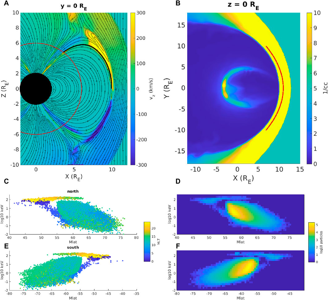
Figure 1. (A) In-plane magnetic field streamlines and
The total number of particles initialized was 300 million with
Given that relatively few particles
One way to collect more particles is to move the inner boundary of the test particle simulation to higher altitude. This allows particles with a greater range of pitch angles at any given energy to hit the inner boundary. Furthermore, the higher the altitude, the less magnetic focusing of the cusp field lines, making it easier to identify overlapping populations that are connected to transient magnetopause dynamics. In this study, the inner boundary radius is 6
3 Overlapping dispersion
The overall dispersion pattern of particles collected at the simulation inner boundary is shown in Figures 1C–F. The scatter plots (Figures 1C, E, northern and southern hemispheres, respectively) show each particle that hit the inner boundary plotted in Mlat-energy space, with the energy axis in logarithmic units and color corresponding to magnetic local time (MLT). In this study, 12 MLT points to the nose of the magnetosphere (the noon meridian) and 0 MLT is in the central magnetotail (the midnight meridian), with 6 MLT and 18 MLT pointing to the top and bottom of Figure 1B, respectively, and corresponding to the dawn and dusk terminators. Figures 1C, E show 2 distinct populations separated by day-side (6–18 MLT, blue-green colors) and night-side (18–24 and 0–6 MLT, yellow and dark blue colors) MLT sectors. The spectrograms in Figures 1D, F show the corresponding particle counts in the same Mlat-energy bins. Particles hitting the inner boundary on the day-side have a standard dispersion signature, with the highest energy particles at lower absolute Mlats. All particles that hit the inner boundary over the course of the simulation are collected for these spectrograms. Therefore, they represent a time-averaged dispersion that smooths out structures associated with dynamics of the day-side x-line, which occur on a time scale of a few minutes in this simulation (Burkholder et al., 2023). The day-side flux ropes, for instance, move from the equator into the cusp on a time scale of
To construct synthetic dispersion signatures that can be compared to Earth orbiting satellites, synthetic spacecraft are launched with constant values of MLT at an altitude of 6
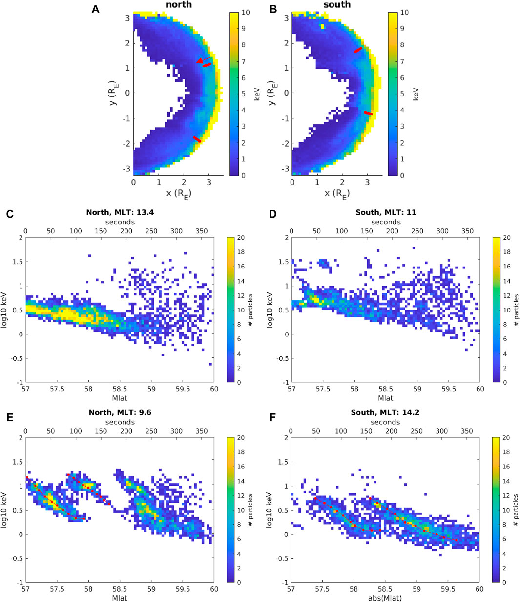
Figure 2. Colormaps show the (A) Northern and (B) Southern hemisphere average energy of precipitated particles at the inner boundary (6
Synthetic observations at the example MLTs are shown in Figures 2C–F. Figures 2C, D show between absolute Mlats of 57 and 58.5°, the energy of ions decreases steadily. These are examples of standard dispersion during southward IMF. These correspond to the trajectories taken at MLT 13.4 in the northern hemisphere (Figure 2C) and MLT 11 in the southern hemisphere (Figure 2D). Figures 2E, F show examples of overlapping dispersions in the northern (MLT 9.8) and southern hemispheres (MLT 14.2), respectively. The red dots, which will be discussed alongside Figure 8, are plotted through the central portion of nonzero fluxes, which is not necessarily the highest flux at each Mlat but it is generally close. The dispersions are standard in the sense that the energy of both populations decreases with increasing absolute Mlat. The defining feature is the region of overlap with a near absence of particles at energies between the two populations. The distance of the overlap is
Figure 3 examines the two populations of particles that produced the overlapping dispersion in Figure 2E. Figure 3A shows the individual particles that were collected from 57 to 58.3° Mlat. The color indicates whether the particle belongs to the lower (blue) or higher (green) energy population of the overlapping dispersion, which were separated based on the red line. These terms “lower” and “higher” will be used hereafter to refer to the dispersion containing the lower or higher energy particles in the region of overlap. Following the same color scheme, Figure 3B plots each particle where it hit the inner boundary of the test particle simulation. It is clear that there is a region where the two populations are co-located, which serves to demonstrate that the two populations in Figure 2E are overlapping rather than only appearing so due to the finite size binning. A blue particle and a green particle have been singled out with magenta star markers. Figure 3A shows that these two particles hit the inner boundary at the same Mlat in the overlapping region of the dispersion. In Figure 3B the same particles can be identified by magenta stars with colored points representing the blue or green population. Figure 3B shows that the spatial separation of the starred particles at the inner boundary is
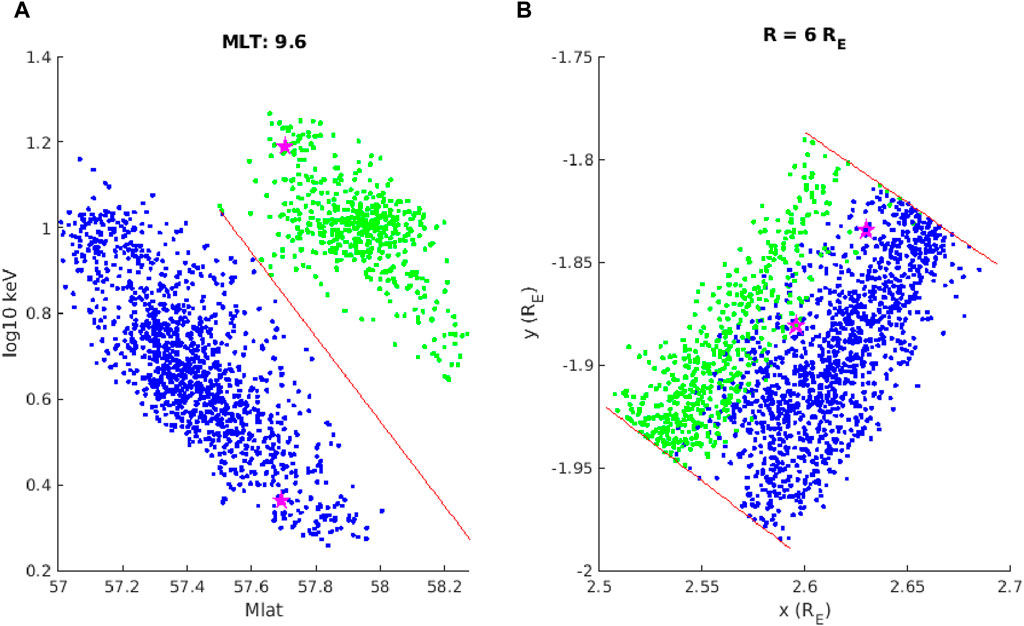
Figure 3. (A) Individual particles, plotted on Mlat-energy axes, that were collected by the synthetic satellite in Figure 2E from 57 to 58.3° Mlat (energy axis is in logarithmic units). The red line separates the two overlapping populations with the higher energy population colored green and the lower energy population colored blue. (B) Plots all the same particles at their location of precipitation at the inner boundary (in SM coordinates). The red lines show the size of the MLT bins. This demonstrates that the overlapping populations are co-located in coordinate space, not just appearing so in Mlat-energy space because of finite sized binning. Particles with a star marker are examined in Figures 4, 5.
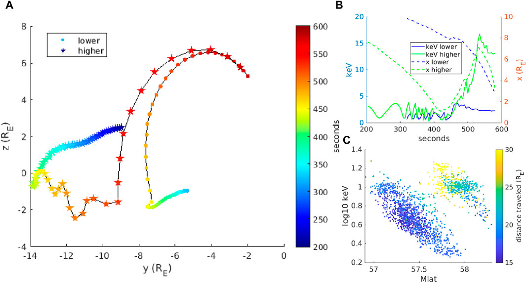
Figure 4. (A) Trajectories viewed in the
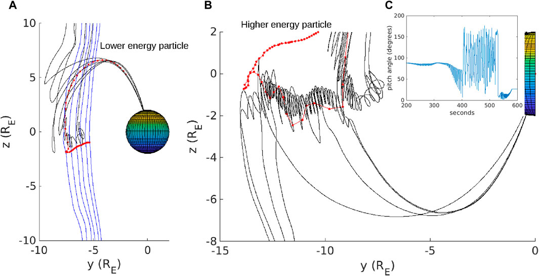
Figure 5. (A) Three-dimensional magnetic field lines traced from the lower energy particle location as it moved from its initial location to the inner boundary. Blue represents magnetosheath magnetic field with no connection to the simulation inner boundary, and black represents open magnetic field with only 1 end connected to the inner boundary. (B) Three-dimensional magnetic field lines at the higher energy particle location. Field lines are only drawn while the particle traverses along the axis of a flux rope and as they enter the cusp. (C) Pitch angle of the higher energy particle, which oscillates between field-aligned and anti-field aligned during the period
Figure 4A shows trajectories projected onto the
Figure 4B shows energy of the two particles as a function of time (solid lines, left axis), along with their x-coordinates (dashed lines, right axis). The colors blue and green correspond to the circles and stars from Figure 4A, respectively (and the colors in Figure 3). The blue particle undergoes an acceleration at t
Figure 5 shows magnetic field lines traced at the location of the two particles along their respective journeys to the inner boundary. The lower energy particle trajectory is shown by the red dots in Figure 5A at 5 s resolution. A field line was traced every 25 s and the color of the field line corresponds to magnetosheath (blue) or connected to the inner boundary at 1 end only (black). As the particle moved initially in the
The higher energy particle trajectory is shown by the red dots in Figure 5B. As the particle initially moved from y
Notice, magnetic field lines comprising the flux rope in Figure 5B have one end connected to the southern hemisphere inner boundary and the other end open to the magnetosheath. It is not trivial to see how particles trapped in this flux rope can end up in the northern cusp. The key aspect of the magnetic flux rope is that all types of magnetic topology exist within the flux rope (Pu et al., 2013; Zhong et al., 2013, see also Burkholder et al., 2023 Figure 6). Reconnection can occur between open field lines (one end connected to the inner boundary) and closed field lines (connected to both northern and southern hemispheres) which are twisted around the flux rope. This type of reconnection allows particles which are initially trapped in the flux rope to precipitate in the northern hemisphere cusp. Particles accelerated in the flux rope are thus able to access the same flux tube where an earlier population of less energetic particles, like Figure 5A, precipitated on.
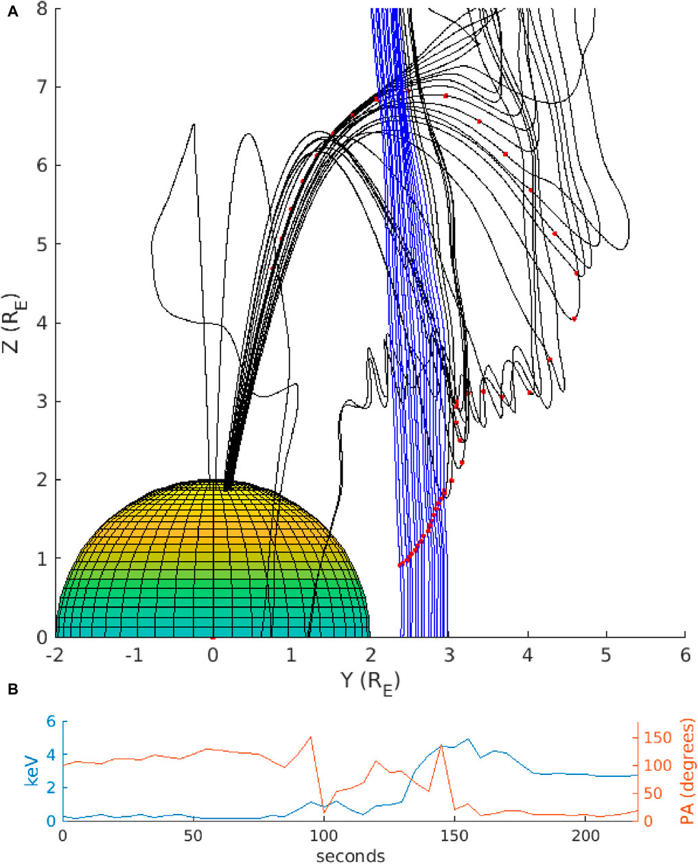
Figure 6. (A) Three-dimensional magnetic field lines traced from a particle location (red dot) having initial energy 0.1 keV and initial pitch angle 100°. Blue and black magnetic field lines represent the same magnetic connections as Figure 5. (B) Energy (blue, left axis) and pitch angle (orange, right axis) evolution of the particle. The energy increase occurs while the pitch angle oscillates between field-aligned and anti-field-aligned, the same motion as the particle in Figure 5B executes while traversing the flux rope.
Figure 6 shows another example of an ion test particle traversing the axis of a flux rope. This particle was not part of the simulation described in Section 2, but was from a testing run performed to confirm the robustness of this paper’s conclusions against different particle initializations. Essentially every aspect of this simulation was the same as described in Section 2 except there were only 10 million total particles and the initial energy was 0.1 keV. This specific particle was chosen because it precipitated into the northern cusp with a population of particles that form the higher energy portion of an overlapping dispersion. Figure 6A shows the ion was initially on a magnetosheath field line (blue), and eventually accessed an open field line (black) with 1 end connected to the inner boundary. The first open field line that the particle accessed was not part of a magnetic flux rope, but after about 20 s the particle trajectory became confined to a magnetic flux rope. The particle eventually escaped the flux rope and traveled into the northern cusp on a poleward convecting open field line. Figure 6B shows the energy (left-side blue axis) and pitch angle (right-side orange axis) for this particle. During the acceleration interval from
4 Comparison of simulation and DMSP
Figures 7A, C show observations from Special Sensor J (SSJ) on the DMSP F16 satellite (Redmon et al., 2017). The instrument gives ion differential energy flux in the range 30 eV to 30 keV, at a nominal altitude of 850 km. These events were taken from the database of overlapping dispersions identified by da Silva et al. (2024). They were chosen specifically because the IMF is strongly southward in both instances (see Figures 7B, D titles), as drawn from the OMNIWeb data product. They were also both observed in the day-side cusp region (near 14 MLT for event 1 and 12 MLT for event 2), similar to the synthetic observations in Figure 2. The blue and green lines in Figures 7A, C, corresponding to the two overlapping populations, were drawn to trace the lower and upper dispersions, respectively. The region of overlap lies between the vertical dashed lines. In Figure 7A the overlap is
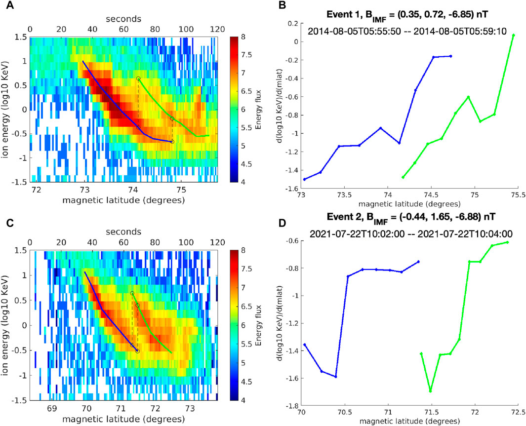
Figure 7. (A,C) Two examples of overlapping dispersions observed by DMSP during strongly southward IMF. The blue (green) line was drawn through the region of highest flux at each Mlat for the lower (higher) energy population of the overlapping dispersion. The vertical dashed lines show the region of overlap. (B,D) The corresponding local slopes of the green and blue lines drawn in (A,C).
The slope of the overlapping dispersions in Mlat-energy space can also be compared from the simulation and observation. Lockwood and Smith (1992) showed that the slope of the dispersion could be related to the upstream reconnection rate at the magnetopause. Figures 7B, D show the slope as a function of Mlat for the DMSP observations, with blue and green lines giving the slope corresponding to the blue and green lines in Figures 7A, C. Locally, the slopes are somewhat variable but the general trend is that the slope gets shallower with increasing Mlat. In both instances the lower portion (blue) of the overlapping dispersions have an average slope of about 1 order of magnitude keV per degree Mlat and for the higher portion (green) it is only slightly shallower.
The slopes of the synthetic overlapping dispersions were also calculated (see red dots in Figures 2E, F, similar to the blue and green lines in Figures 7A, C) and the comparison with DMSP observations is shown in Figure 8. The slopes are given as a function of energy (on a logarithmic scale). The slopes for the lower portions of the overlapping dispersions are plotted in Figure 8A and the slopes of the upper portions are plotted in Figure 8B. The blue and black lines in Figure 8A show the local slopes for the lower portions of the simulation dispersions. These have a trend of steeper slope at higher energy, the same as DMSP (red and green). The upper portion of the simulation dispersions (Figure 8B) shows steeper slopes at higher energy for black (corresponding to Figure 2F), comparing well with red and green. The blue slopes (corresponding to Figure 2E) are fairly constant (about 1 order of magnitude keV per degree Mlat) through their entire energy range. This is probably because there were few particles collected for this dispersion with
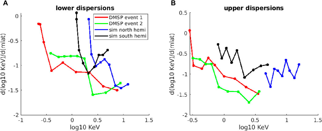
Figure 8. (A) Slope as a function of energy for lower portions of the simulated and observed overlapping dispersion signatures. Black and blue are calculated from the simulated overlapping dispersions in Figures 2E, F, respectively. Green and red are calculated from the observed overlapping dispersions in Figures 7A, C, respectively. (B) Slope as a function of energy for upper portions of the simulated and observed overlapping dispersion signatures, with same colors as (A). Energy axes are in logarithmic units.
Another quantity to compare is the energy separation of the overlapping populations. It is about 15 keV for Figure 2E and 4 keV for Figure 2F, compared to
5 Summary and discussion of conclusion
The global MHD with test particle approximation was employed to understand the origin of overlapping cusp ion dispersion signatures during steady strongly southward IMF. It was found that different satellite paths through the cusp give different dispersion signatures, with some having overlapping populations and others having the standard dispersion (for southward IMF). By examining the trajectory of a particle in each population of an overlapping dispersion, it was determined that the higher energy population is formed by particles traversing the axis of a flux rope before going into the cusp. Particles from the lower energy population travel more directly from a magnetosheath field line into the cusp without being trapped. Trapped particles are energized as they gyrate across the magnetopause current sheet, accessing both magnetosphere and magnetosheath fields which have a magnetic shear angle of
Different acceleration histories for energy-separated populations which end up on the same open magnetic flux tube is a fundamentally new physical mechanism to account for overlapping dispersions. The existing interpretation of overlapping dispersions has different energy populations which underwent a similar acceleration history. That mechanism invokes the existence of multiple reconnection sites on the same open magnetic flux tube, leading to multiple injection events (Lockwood, 1995). The initial reconnection existed longer, and thus injects a lower energy population. A secondary reconnection of the same flux tube field lines, more recently been initiated, injects a higher energy population. Despite this difference, the formation of magnetic flux ropes and the magnetic topology changes that allow particles to escape flux ropes are also secondary reconnection processes, so it is the case that both the new and existing mechanisms rely on multiple reconnection of the same flux tube field lines. Missions targeting the day-side magnetopause, like NASA’s Magnetospheric Multiscale (MMS), may be able to determine the properties of particles traversing flux ropes and confirm whether the new mechanism is occurring. Otherwise, it is possible that flux ropes in global MHD simulation are not sufficiently realistic or the particles escape them via some kinetic processes not resolved in the test particle approximation.
Even these two mechanisms (traditional multiple reconnection of the same flux tube field lines, described above, and flux rope traversal, the subject of this paper) are unlikely to account for all observed overlapping dispersions, especially given the range of solar wind and IMF conditions that can impact Earth. There are different ways that multiple reconnection can occur, such as local flux tube interchange (Ma et al., 2019) associated with the Kelvin-Helmholtz instability (most likely near the flank regions) and interlinked flux tube reconnection (Cardoso et al., 2013; Øieroset et al., 2019). The observation and simulation comparisons in this study show remarkable similarity, but future work is needed to determine observational differences in overlapping dispersions caused by different multiple reconnection processes. Furthermore there is also the possibility that particles sourced elsewhere than the magnetosheath and solar wind play a role in the formation of overlapping dispersion signatures. For instance, particles trapped in the cusp diamagnetic cavity can escape due to magnetic topology changes (Nykyri et al., 2011; Nykyri et al., 2012; Burkholder et al., 2021) and if they end up deeper in the cusp they may be overlapping with a solar wind population when they precipitate, depending on how much energy was gained in the diamagnetic cavity.
Data availability statement
The datasets presented in this study can be found in online repositories. The names of the repository/repositories and accession number(s) can be found in the article/supplementary material.
Author contributions
BB: Conceptualization, Data curation, Formal Analysis, Funding acquisition, Investigation, Methodology, Project administration, Resources, Software, Supervision, Validation, Visualization, Writing–original draft, Writing–review and editing. YG: Formal Analysis, Investigation, Writing–review and editing. AP: Data curation, Formal Analysis, Investigation, Visualization, Writing–review and editing. L-JC: Conceptualization, Writing–review and editing. JD: Writing–review and editing. XM: Writing–review and editing. DD: Writing–review and editing. HC: Writing–review and editing. SP: Writing–review and editing.
Funding
The author(s) declare that financial support was received for the research, authorship, and/or publication of this article. This work is provided by NASA Magnetospheric Multiscale (MMS) Early Career Grant 80NSSC22K0949.
Acknowledgments
We acknowledge use of NASA/GSFC’s Space Physics Data Facility’s OMNIWeb, and also the Texas Advanced Computing Center (TACC) at The University of Texas at Austin for providing HPC resources that have contributed to the research results reported within this paper http://www.tacc.utexas.edu. We thank the team of the Center for Geospace Storms for providing the MAGE model.
Conflict of interest
The authors declare that the research was conducted in the absence of any commercial or financial relationships that could be construed as a potential conflict of interest.
The author(s) declared that they were an editorial board member of Frontiers, at the time of submission. This had no impact on the peer review process and the final decision.
Publisher’s note
All claims expressed in this article are solely those of the authors and do not necessarily represent those of their affiliated organizations, or those of the publisher, the editors and the reviewers. Any product that may be evaluated in this article, or claim that may be made by its manufacturer, is not guaranteed or endorsed by the publisher.
References
Basinska, E. M., Burke, W. J., Maynard, N. C., Hughes, W. J., Winningham, J. D., and Hanson, W. B. (1992). Small-scale electrodynamics of the cusp with northward interplanetary magnetic field. J. Geophys. Res. Space Phys. 97, 6369–6379. doi:10.1029/91JA03023
Burkholder, B. L., Chen, L.-J., Sorathia, K., Sciola, A., Merkin, S., Trattner, K. J., et al. (2023). The complexity of the day-side x-line during southward interplanetary magnetic field. Front. Astronomy Space Sci. 10. doi:10.3389/fspas.2023.1175697
Burkholder, B. L., Nykyri, K., Ma, X., Sorathia, K., Michael, A., Otto, A., et al. (2021). The structure of the cusp diamagnetic cavity and test particle energization in the gamera global mhd simulation. J. Geophys. Res. Space Phys. 126, e2021JA029738. doi:10.1029/2021JA029738
Cardoso, F. R., Gonzalez, W. D., Sibeck, D. G., Kuznetsova, M., and Koga, D. (2013). Magnetopause reconnection and interlinked flux tubes. Ann. Geophys. 31, 1853–1866. doi:10.5194/angeo-31-1853-2013
Connor, H. K., Raeder, J., Sibeck, D. G., and Trattner, K. J. (2015). Relation between cusp ion structures and dayside reconnection for four imf clock angles: openggcm-ltpt results. J. Geophys. Res. Space Phys. 120, 4890–4906. doi:10.1002/2015JA021156
da Silva, D., Chen, L. J., Fuselier, S., Wang, S., Elkington, S., Dorelli, J., et al. (2022). Automatic identification and new observations of ion energy dispersion events in the cusp ionosphere. J. Geophys. Res. Space Phys. 127, e2021JA029637. doi:10.1029/2021JA029637
da Silva, D. E., Chen, L. J., Fuselier, S. A., Petrinec, S. M., Trattner, K. J., Cucho-Padin, G., et al. (2024). Statistical analysis of overlapping double ion energy dispersion events in the northern cusp. Front. Astronomy Space Sci. 10. doi:10.3389/fspas.2023.1228475
Fuselier, S. A., Kletzing, C. A., Petrinec, S. M., Trattner, K. J., George, D., Bounds, S. R., et al. (2022). Multiple reconnection x-lines at the magnetopause and overlapping cusp ion injections. J. Geophys. Res. Space Phys. 127, e2022JA030354. doi:10.1029/2022JA030354
Fuselier, S. A., Petrinec, S. M., Trattner, K. J., Broll, J. M., Burch, J. L., Giles, B. L., et al. (2018). Observational evidence of large-scale multiple reconnection at the earth’s dayside magnetopause. J. Geophys. Res. Space Phys. 123, 8407–8421. doi:10.1029/2018JA025681
Grandin, M., Turc, L., Battarbee, M., Ganse, U., Johlander, A., Pfau-Kempf, Y., et al. (2020). Hybrid-Vlasov simulation of auroral proton precipitation in the cusps: comparison of northward and southward interplanetary magnetic field driving. J. Space Weather Space Clim. 10, 51. doi:10.1051/swsc/2020053
Lavraud, B., and Trattner, K. J. (2021). The polar cusps of the earth’s magnetosphere. American Geophysical Union AGU 11, 163–176. doi:10.1002/9781119815624.ch11
Lockwood, M. (1995). Overlapping cusp ion injections: an explanation invoking magnetopause reconnection. Geophys. Res. Lett. 22, 1141–1144. doi:10.1029/95GL00811
Lockwood, M., and Smith, M. F. (1989). Low-altitude signatures of the cusp and flux transfer events. Geophys. Res. Lett. 16, 879–882. doi:10.1029/GL016i008p00879
Lockwood, M., and Smith, M. F. (1992). The variation of reconnection rate at the dayside magnetopause and cusp ion precipitation. J. Geophys. Res. Space Phys. 97, 14841–14847. doi:10.1029/92JA01261
Ma, X., Delamere, P. A., Thomsen, M. F., Otto, A., Neupane, B., Burkholder, B., et al. (2019). Flux tube entropy and specific entropy in saturn’s magnetosphere. J. Geophys. Res. Space Phys. 124, 1593–1611. doi:10.1029/2018JA026150
Merkin, V. G., and Lyon, J. G. (2010). Effects of the low-latitude ionospheric boundary condition on the global magnetosphere. J. Geophys. Res. Space Phys. 115. doi:10.1029/2010JA015461
Nykyri, K., Otto, A., Adamson, E., Dougal, E., and Mumme, J. (2011). Cluster observations of a cusp diamagnetic cavity: structure, size, and dynamics. J. Geophys. Res. (Space Phys.) 116, A03228. doi:10.1029/2010JA015897
Nykyri, K., Otto, A., Adamson, E., Kronberg, E., and Daly, P. (2012). On the origin of high-energy particles in the cusp diamagnetic cavity. J. Atmos. Solar-Terrestrial Phys. 87-88, 70–81. doi:10.1016/j.jastp.2011.08.012
Øieroset, M., Phan, T. D., Drake, J. F., Eastwood, J. P., Fuselier, S. A., Strangeway, R. J., et al. (2019). Reconnection with magnetic flux pileup at the interface of converging jets at the magnetopause. Geophys. Res. Lett. 46, 1937–1946. doi:10.1029/2018GL080994
Pitout, F., and Bogdanova, Y. V. (2021). The polar cusp seen by cluster. J. Geophys. Res. Space Phys. 126, e2021JA029582. doi:10.1029/2021JA029582
Pitout, F., Escoubet, C. P., Klecker, B., and Dandouras, I. (2009). Cluster survey of the mid-altitude cusp - part 2: large-scale morphology. Ann. Geophys. 27, 1875–1886. doi:10.5194/angeo-27-1875-2009
Pitout, F., Escoubet, C. P., Taylor, M. G. G. T., Berchem, J., and Walsh, A. P. (2012). Overlapping ion structures in the mid-altitude cusp under northward imf: signature of dual lobe reconnection? Ann. Geophys. 30, 489–501. doi:10.5194/angeo-30-489-2012
Pu, Z. Y., Raeder, J., Zhong, J., Bogdanova, Y. V., Dunlop, M., Xiao, C. J., et al. (2013). Magnetic topologies of an in vivo fte observed by double star/tc-1 at earth’s magnetopause. Geophys. Res. Lett. 40, 3502–3506. doi:10.1002/grl.50714
Redmon, R. J., Denig, W. F., Kilcommons, L. M., and Knipp, D. J. (2017). New dmsp database of precipitating auroral electrons and ions. J. Geophys. Res. Space Phys. 122, 9056–9067. doi:10.1002/2016ja023339
Sorathia, K. A., Merkin, V. G., Panov, E. V., Zhang, B., Lyon, J. G., Garretson, J., et al. (2020). Ballooning-interchange instability in the near-earth plasma sheet and auroral beads: global magnetospheric modeling at the limit of the mhd approximation. Geophys. Res. Lett. 47, e2020GL088227. doi:10.1029/2020GL088227
Sorathia, K. A., Merkin, V. G., Ukhorskiy, A. Y., Mauk, B. H., and Sibeck, D. G. (2017). Energetic particle loss through the magnetopause: a combined global mhd and test-particle study. J. Geophys. Res. Space Phys. 122, 9329–9343. doi:10.1002/2017JA024268
Sorathia, K. A., Ukhorskiy, A. Y., Merkin, V. G., Fennell, J. F., and Claudepierre, S. G. (2018). Modeling the depletion and recovery of the outer radiation belt during a geomagnetic storm: combined mhd and test particle simulations. J. Geophys. Res. Space Phys. 123, 5590–5609. doi:10.1029/2018JA025506
Speiser, T. W. (1965). Particle trajectories in model current sheets: 1. analytical solutions. J. Geophys. Res. (1896-1977) 70, 4219–4226. doi:10.1029/JZ070i017p04219
Speiser, T. W. (1967). Particle trajectories in model current sheets: 2. applications to auroras using a geomagnetic tail model. J. Geophys. Res. (1896-1977) 72, 3919–3932. doi:10.1029/JZ072i015p03919
Tan, B., Lin, Y., Perez, J. D., and Wang, X. Y. (2012). Global-scale hybrid simulation of cusp precipitating ions associated with magnetopause reconnection under southward imf. J. Geophys. Res. Space Phys. 117. doi:10.1029/2011JA016871
Trattner, K. J., Coates, A. J., Fazakerley, A. N., Johnstone, A. D., Balsiger, H., Burch, J. L., et al. (1998). Overlapping ion populations in the cusp: polar/timas results. Geophys. Res. Lett. 25, 1621–1624. doi:10.1029/98GL01060
Trattner, K. J., Petrinec, S. M., Fuselier, S. A., Omidi, N., and Sibeck, D. G. (2012). Evidence of multiple reconnection lines at the magnetopause from cusp observations. J. Geophys. Res. Space Phys. 117. doi:10.1029/2011JA017080
Xiong, Y.-T., Han, D.-S., Wang, Z.-w., Shi, R., and Feng, H.-T. (2024). Intermittent lobe reconnection under prolonged northward interplanetary magnetic field condition: insights from cusp spot event observations. Geophys. Res. Lett. 51, e2023GL106387. doi:10.1029/2023GL106387
Zhang, B., Sorathia, K. A., Lyon, J. G., Merkin, V. G., Garretson, J. S., and Wiltberger, M. (2019). GAMERA: a three-dimensional finite-volume MHD solver for non-orthogonal curvilinear geometries. Astrophysical J. Suppl. Ser. 244, 20. doi:10.3847/1538-4365/ab3a4c
Keywords: cusp dispersion, ion dynamics, magnetic reconnection, flux transfer events, global simulation, magnetohydrodynamics, test particles, magnetic flux ropes
Citation: Burkholder BL, Girma Y, Porter A, Chen L-J, Dorelli J, Ma X, Da Silva D, Connor H and Petrinec S (2024) Overlapping cusp ion dispersions formed by flux ropes on the day-side magnetopause. Front. Astron. Space Sci. 11:1430966. doi: 10.3389/fspas.2024.1430966
Received: 10 May 2024; Accepted: 08 August 2024;
Published: 21 August 2024.
Edited by:
Elena Kronberg, Ludwig Maximilian University of Munich, GermanyReviewed by:
Yulia Bogdanova, Rutherford Appleton Laboratory, United KingdomRobert Fear, University of Southampton, United Kingdom
Copyright © 2024 Burkholder, Girma, Porter, Chen, Dorelli, Ma, Da Silva, Connor and Petrinec. This is an open-access article distributed under the terms of the Creative Commons Attribution License (CC BY). The use, distribution or reproduction in other forums is permitted, provided the original author(s) and the copyright owner(s) are credited and that the original publication in this journal is cited, in accordance with accepted academic practice. No use, distribution or reproduction is permitted which does not comply with these terms.
*Correspondence: Brandon L. Burkholder, YmxidXJraG9sZGVyQGFsYXNrYS5lZHU=