Intermediate E-F layer dynamics study in the Brazilian low-latitude sector: observational data and simulations

This study investigates the downward motion of Intermediate E-F Layers (ILs) in the Brazilian low latitude sector through observation and modeling. Ionosonde data from São José dos Campos (SJC) and Palmas (PAL) were analyzed to investigate the seasonal variation of the IL parameters, including the virtual height (h'IL) and the top frequency (ftIL). The ILs primarily originated from F layer detachment followed by downward motion, peaking before 11 LT and disappearing well before sunset. Daily height variability ranged between 130 and 190 km, with peak frequencies around 4–5 MHz. Using meteor radar data as input, the Ionospheric E-region Model (MIRE) simulated diurnal and semidiurnal tides to analyze neutral wind effects on ILs descent. Model simulations for SJC (October 2008) and PAL (April and June 2009) revealed distinct wind oscillations influencing IL dynamics at heights below 140 km. In SJC, meridional wind shears controlled IL descent, with possible zonal wind interactions weakening ILs. Conversely, in PAL during April 2009, both zonal and meridional winds contributed to IL formation and altitude descent. However, discrepancies between observed and modeled descent rates suggest the need for considering additional atmospheric wave interactions in future modeling studies. June 2009 over PAL presented unique IL behavior, exhibiting a lower observed decay rate and daily height oscillations potentially linked to local modulations. Meanwhile, MIRE indicated that meridional wind shearing predominantly controlled IL descent in the morning, with zonal wind becoming relevant post-midday. These findings enhance our understanding of IL dynamics and their atmospheric drivers.

1 Introduction

Intermediate E-F Layers (ILs), also known as intermediate descending layers, or simply intermediate layers, are thin and enhanced ionization regions that form between the top of the E region and the bottom side of the F region at altitudes between around 150–200 km. The ILs tend to have a descending motion through the ionospheric E-F valley region with velocities that may attain values between 0.3 and 12.5 m.s⁻¹ (Niranjan et al., 2010; Santos et al., 2020; Oikonomou et al., 2023). The vertical shear of the horizontal neutral winds (ion convergence) is the most accepted mechanism to explain the formation of the ILs (Wilkinson et al., 1992; Osterman et al., 1995). As the ILs move down to lower heights, they can merge with the high type of sporadic-E (Es_h) layer (120–150 km) and may also play an important role in the generating processes of lower-altitude Es layers (100–120 km) (Szuszczewicz et al., 1995; Haldoupis, 2012).

Observations of ILs have been reported for over seven decades by using different ground-based experimental techniques such as ionosondes (Rodger et al., 1981; Wilkinson et al., 1992; Watts and Brown, 1994; Niranjan et al., 2010; Dos Santos et al., 2019; Santos et al., 2022) and radars (Kudeki and Fawcett, 1993; Rowe, 1993; Earle et al., 2000). Most of these investigations were conducted in mid-latitude regions, which led to a current understanding of the processes involved in the formation and dynamics of these layers. However, with the advent of satellite measurements, it was possible to observe that when the ILs form, their chemical composition is entirely made up of the molecular ions NO⁺ and O₂⁺ (Miller et al., 1993). As the ILs descend to lower altitudes, their composition also shows a combination of metallic ions, such as Fe⁺ and Mg⁺ (Earle et al., 2000). Eventually, they may become entirely comprised of metal ions.

Although the ILs have been extensively investigated at mid-latitudes, more relevant observational studies of these layers in equatorial and low latitude regions have started to emerge in recent years. To study the diurnal and seasonal variations of ILs and their relationships with tidal motions, Lee et al. (2003) analysed 1 year of digisonde data collected at a low-latitude station in the Taiwanese sector. Based on the diurnal distributions of the occurrence probability of ILs, they estimated that the semidiurnal (quarter-diurnal) tide was the dominant component during the spring/winter (summer/autumn) seasonal periods. In the South American sector, the first climatologic study of ILs was reported by Dos Santos et al. (2019). The authors analysed 1 year of data with ILs’ traces in the ionograms recorded by the ionosondes installed at the equatorial station of São Luís (2°S; 44°W), and at the low latitude station of Cachoeira Paulista (22.42° S; 45°W). The observations were conducted around the year of extremely low solar activity in 2009. The ILs were observed during 90% and 60% of the days with available data at Cachoeira Paulista and São Luis, respectively. Although they were predominantly observed during the daytime, Dos Santos et al. (2019) also reported cases of IL at night, simultaneous ILs at different altitudes, and, more rarely, the occurrence of ascending layers. However, such ascending layers were recently related to the normal evening F layer vertical rise due to the prereversal enhancement (PRE) of the zonal electric field (Santos et al., 2021). When comparing the results obtained at São Luís and Cachoeira Paulista with observations conducted close to the solar maximum year of 2003, Santos et al. (2020) noted that the lifetime (duration) of the ILs during the year of solar minimum (2009) was higher than in the solar maximum (2003). Regarding the descending motion of the ILs, Santos et al. (2020) suggested that they are mainly controlled by the semidiurnal and quarter-diurnal tidal oscillations. Over the equatorial site of São Luís, the larger descending rate in some cases (>10 km/h) also indicated the possible influence of the gravity waves in the dynamics of the ILs. In the Indian equatorial site of Thiruvananthapuram (8.5°N; 77°E), Mridula and Pant (2022) analysed 8 years of ionosonde observations and reported a higher occurrence of ILs during summer and winter solstice months against minima during equinoxes. Analogous to the observations over the Brazilian sector by Santos et al. (2020), they found that the probability of ILs’ occurrence is higher during the solar minimum period than during the solar maximum period. More recently, Shaik et al. (2024) revealed from height-time-intensity (HTI) technique the effects of tide like periodicities on the dynamics of ILs at a low-mid latitude station located in the Arabian sector.

In terms of modeling of the ILs, several studies have been carried out in the past 50 years. Fujitaka and Tohmatsu (1973) solved the time-dependent continuity equation by analysing charge transport effects and concluded that the ILs result primarily from the wind shear process, mainly due to the semidiurnal tidal oscillation in the thermosphere. A study performed by Wilkinson et al. (1992) employed the NCAR TIGCM (Thermospheric-Ionospheric Global Circulation Model) and compared the simulation results with ionosonde observations conducted at the Australian mid-latitude region. They showed that the shearing in the meridional component of the neutral winds was more effective in producing the layering process than the zonal wind. Moreover, they argued that the day-to-day variability of the ILs might result from variations in the tidal winds, electric fields, or metallic ion composition. Osterman et al. (1995) modelled the formation of ILs at Arecibo by employing the Bailey Ionospheric Model (Bailey and Sellek, 1990), and showed that tidal-like meridional wind profiles act to their plasma density enhancement. Szuszczewicz et al. (1995) identified from simulations of the NCAR Thermosphere-Ionosphere-Electrodynamics (TIE-GCM) model that the 24-, 12-, and 8-h tidal modes, controlled by the shears in the meridional and zonal winds, were the causal mechanisms for ILs’ formation and transport. Bishop and Earle (2003) used a model developed specifically to investigate the formation mechanisms and dynamics of ILs at mid-latitudes. They showed that at higher altitudes (above 130 km) where the ILs are formed, the meridional wind component is more efficient in affecting the ion motion owing to the very small ratio between collision frequency and gyro frequency. Furthermore, the simulations revealed that the metallic ions associated with the ILs are effectively transported downward by increasing the wavelength and amplitude of the imposed horizontal neutral wind component.

However, it is noteworthy that there is a lack of studies on modeling the intermediate layers in the ionosphere for low-latitude regions. With this in mind, the present work investigates the characteristics of the ILs observed by ionosondes installed at two stations located in the Brazilian sector to examine, from numerical simulations, the role of the wind direction on the descending motion of the ILs at low latitudes. Therefore, we employ an extended version of the Ionospheric E-Region Model (MIRE), which incorporates neutral wind data and atmospheric tides inferred from meteor radar data (Resende et al., 2017; Conceição-Santos et al., 2019). Our results allow us to analyze the prevailing wind direction and tidal oscillation affecting ion motion and controlling the descent of the ILs’ altitude down to 140 km.

2 Data and methods

2.1 Ionosonde observations

In this work, we used data recorded from two digital ionosondes that operated simultaneously in the observatories of São José dos Campos (23.2°S; 45.8°W; dip lat. −21.0°), hereafter referred to as SJC, and Palmas (10.2°S; 48.3°W; dip lat. −8.3°), hereafter referred to as PAL. The digital ionosondes used in this work are of the CADI (Canadian Advanced Digital Ionosonde) type. Figure 1 shows the location of the two ionosonde observatories (yellow circles). The CADI system records the ionospheric information in the form of ionograms. In the ionograms the virtual height of the reflected signal echoes versus their frequency (from 1 to 20 MHz) is registered. In this study, the virtual height (h'IL) and the top frequency (ftIL) parameters of the ILs were scaled from the ionograms recorded every 5 min (300 s) at SJC and PAL. The processing of the ionograms and the manual scaling of the IL parameters were performed using the computer software tool named UDIDA (Univap Digital Ionosonde Data Analysis). However, for scaling the h'IL and ftIL parameters from the ionograms we consider the following criteria (Dos Santos et al., 2019): 1. The minimum height for a descending layer to be considered IL was 125 km; 2. The IL parameters were extracted from the extraordinary trace; 3. The descending layer was considered as IL when its critical frequency exceeded the minimum frequency of the ordinary trace of the upper (F layer) region; 4. For the cases of layers formed from the base of the F region, only those that present a total detachment of the F1 layer were classified as IL.

Figure 1

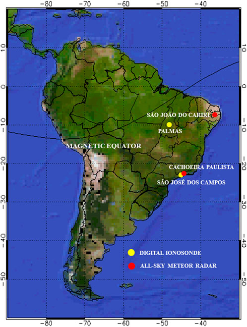
Figure 1. Location of the observatories used in this work for ILs monitoring (São José dos Campos and Palmas) and neutral wind/atmospheric tide estimations (Cachoeira Paulista and São João do Cariri).

The ionosonde data from each observatory were collected during October and December of 2008, and during January, April, June, and July of 2009. We grouped the data collected in the months of June and July of 2009 as representative of winter solstice, October 2008 and April 2009 as representative of equinoxes, and December 2008 and January 2009 as representative of summer solstice. This experiment was conducted during an extremely low solar activity period, when the smoothed sunspot number ranged from 0.3 to 6.6, and the solar radio flux in 10.7 cm (F10.7 index) ranged from ∼65 to 70 sfu. Only data from geomagnetically quiet days with daily (3-hourly planetary) ΣKp < 24 were considered in the analysis.

2.2 Simulations of intermediate layers

This work performed the ILs simulations using a modified version of the Ionospheric E-Region Model (MIRE). This model was originally developed by Carrasco et al. (2007) to simulate the ionospheric electron density at heights from 80 to 140 km. Then, extended versions of the MIRE were presented by Resende et al. (2017) and Conceição-Santos et al. (2019). Recently, the MIRE model has been widely used to study the formation and dynamics of sporadic E-layers in equatorial and low-latitude regions (Conceição-Santos et al., 2020; Resende et al., 2021; Fontes et al., 2023). In this work, the MIRE model was used for the first time to study the dynamics of ILs during their downward movement to altitudes below 140 km towards the E region.

The MIRE algorithm solves a system of equations that describes the chemical and physical processes for the main molecular (${NO}^{+},O_2^{+},{O^{+},N}_2^{+}$) and metallic (${Fe}^{+}$, ${Mg}^{+}$) constituents. Basically, it considers the continuity equation (Eq. 1) and the equation of motion (Eq. 2) for the ionic species as follows:

$\frac{\left.{\partial [\mathbf{N}}_{\mathbf{i}}\right]}{\partial \mathbf{t}}=\mathbf{P}-\mathbf{L}-\frac{\partial \left({\mathbf{V}}_{\mathbf{\text{iz}}}\left[{\mathbf{N}}_{\mathbf{i}}\right]\right)}{\partial \mathbf{z}},(1)$

where $\partial \left[{\mathrm{N}}_{\mathrm{i}}\right]/\partial \mathrm{t}$ is the time derivative of the numerical density of each ionic specie, $\mathrm{P}$ is the production rate per unit volume, $\mathrm{L}$ is the loss rate per unit volume, and $\partial \left({\mathrm{V}}_{\text{iz}}\left[{\mathrm{N}}_{\mathrm{i}}\right]\right)/\partial \mathrm{z}$ denotes the transport term, where ${\mathrm{V}}_{\text{iz}}$ is the vertical velocity of the ions. For the equation of motion, no electric fields are imposed in the present study, as the action of the electric fields on the dynamics of the ILs at low latitude regions is negligible for altitudes below 140 km. Thus, we compute ${\mathrm{V}}_{\text{iz}}$ by considering only the controlling effects of the neutral winds, in agreement with the following equation (Eq. 2):

${\mathit{V}}_{\mathit{i}\mathit{z}}=\frac{{\mathit{\omega }}_{\mathit{i}}^{\mathbf{2}}}{\left({\mathit{\nu }}_{\mathit{i}\mathit{n}}^{\mathbf{2}}+{\mathit{\omega }}_{\mathit{i}}^{\mathbf{2}}\right)}\left[\mathit{c}\mathit{o}\mathit{s}\mathit{I}.\mathit{s}\mathit{i}\mathit{n}\mathit{I}.{\mathit{U}}_{\mathit{x}}+\frac{{\mathit{\nu }}_{\mathit{i}\mathit{n}}}{{\mathit{\omega }}_{\mathit{i}}}.\mathit{c}\mathit{o}\mathit{s}\mathit{I}.{\mathit{U}}_{\mathit{y}}\right],(2)$

where ${\mathrm{\omega }}_{\mathrm{i}}$ is the gyrofrequency, ${\mathrm{v}}_{\text{in}}$ is the ion-neutral collision frequency, I is the magnetic inclination angle, and ${\mathrm{U}}_{\mathrm{x}}$ and ${\mathrm{U}}_{\mathrm{y}}$ are the meridional (positive southward) and zonal (positive eastward) components of the neutral winds, respectively. The subscripts $\mathrm{i}$ and $\mathrm{n}$ refer to the ion and neutral particles, respectively. It is important to mention that the X-axis points towards the south, and the Y-axis indicates towards the east, whereas the Z-axis completes the right-handed coordinate system, pointing up. The equations of the meridional (Eq. 3) and zonal (Eq. 4) wind components are given by:

${\mathit{U}}_{\mathit{x}}\left(\mathit{z}\right)={\mathit{U}}_{\mathit{x}\mathbf{0}}\left(\mathit{z}\right).\mathit{cos}\left(\frac{\mathbf{2}\mathit{\pi }}{{\mathit{\lambda }}_{\mathit{x}}}\left(\mathit{z}-{\mathit{z}}_{\mathbf{0}}\right)+\frac{\mathbf{2}\mathit{\pi }}{\mathit{T}}\left(\mathit{t}-{\mathit{t}}_{\mathit{x}\mathbf{0}}\left(\mathit{z}\right)\right)\right),(3)$

${\mathit{U}}_{\mathit{y}}\left(\mathit{z}\right)={-\mathit{U}}_{\mathit{y}\mathbf{0}}\left(\mathit{z}\right).\mathit{sin}\left(\frac{\mathbf{2}\mathit{\pi }}{{\mathit{\lambda }}_{\mathit{y}}}\left(\mathit{z}-{\mathit{z}}_{\mathbf{0}}\right)+\frac{\mathbf{2}\mathit{\pi }}{\mathit{T}}\left(\mathit{t}-{\mathit{t}}_{\mathit{y}\mathbf{0}}\left(\mathit{z}\right)\right)\right),(4)$

where ${\mathrm{U}}_{\mathrm{x}0,\mathrm{y}0}\left(\mathrm{z}\right)$ are the wind amplitudes at height z, ${\mathrm{\lambda }}_{\mathrm{x},\mathrm{y}}$ are the vertical wavelengths, ${\mathrm{t}}_{\mathrm{x}0,\mathrm{y}0}\left(\mathrm{z}\right)$ are the wave phases at height z, ${\mathrm{z}}_0$ is the reference height (${\mathrm{z}}_0$ = 100 km), and T is the tidal period, which can be diurnal (24-h) or semidiurnal (12-h) for the simulations considered here.

In this study, the parameters of the diurnal and semidiurnal tides, as well as the values of ${\mathrm{U}}_{\mathrm{x}0,\mathrm{y}0}$, ${\mathrm{\lambda }}_{\mathrm{x},\mathrm{y}}$, and ${\mathrm{t}}_{\mathrm{x}0,\mathrm{y}0}$ were computed from data collected by the meteor radars installed in the stations of Cachoeira Paulista (22.4°S; 45.0°W; dip lat. −21.1°) and São João do Cariri (7.2°S; 36.3°W; dip lat. −12.2). The locations of the meteor radar observatories are also shown in Figure 1 (red circles). The meteor radars used in this work are of the type SKiYMET (All-Sky Interferometric Meteor Radar). Therefore, SKiYMET radar data were used to infer the neutral winds and atmospheric tides in the height ranging from 86 to 100 km. However, as the height of interest in this study is up to 100 km, we used a modified version of MIRE to obtain a more realistic wind profile. The modifications incorporated into MIRE model were as follows (Conceição-Santos et al., 2019; Fontes et al., 2023): 1. Meridional and zonal wind amplitudes were extrapolated with a Lorentz curve fitting for heights from 100 to 140 km; 2. ${\lambda }_{x,y}$ was considered constant from 100 to 120 km; 3. ${\lambda }_{x,y}$ was adjusted tending to infinity between 120 and 140 km; 4. The inclusion of seasonal variability of the metallic ions. The SKiYMET wind profiles obtained from data collected at Cachoeira Paulista were used as input to the MIRE model to represent the winds over the observatory of SJC, whereas the wind data collected at São João do Cariri were used as representative of the winds over PAL.

For the production (P) and loss (L) terms in Eq. 1, the continuity equations for each of the ionic species are obtained from the chemical reactions (Eqs 5–10) in the ionosphere at heights from 80 to 140 km:

$\left[{\mathit{O}}^{+}\right]=\frac{{\mathit{q}}_{{\mathit{O}}^{+}}}{{\mathit{\kappa }}_{\mathbf{1}}\left[{\mathit{O}}_{\mathbf{2}}\right]+{\mathit{\kappa }}_{\mathbf{2}}\left[{\mathit{N}}_{\mathbf{2}}\right]},(5)$

$\left[{\mathit{N}}_{\mathbf{2}}^{+}\right]=\frac{{\mathit{q}}_{{\mathit{N}}_{\mathbf{2}}^{+}}}{{\mathit{\kappa }}_{\mathbf{3}}\left[\mathit{O}\right]+{\mathit{\kappa }}_{\mathbf{4}}\left[{\mathit{O}}_{\mathbf{2}}\right]},(6)$

$\begin{array}{l}\frac{\partial \left[{\mathit{O}}_{\mathbf{2}}^{+}\right]}{\partial \mathit{t}}={\mathit{q}}_{{\mathit{O}}_{\mathbf{2}}^{+}}+{\mathit{\kappa }}_{\mathbf{1}}\left[{\mathit{O}}^{+}\right]\left[{\mathit{O}}_{\mathbf{2}}\right]+{\mathit{\kappa }}_{\mathbf{4}}\left[{\mathit{N}}_{\mathbf{2}}^{+}\right]\left[{\mathit{O}}_{\mathbf{2}}\right]-{\mathit{\kappa }}_{\mathbf{5}}\left[{\mathit{O}}_{\mathbf{2}}^{+}\right]\left[\mathit{N}\mathit{O}\right]\\ -{\mathit{\alpha }}_{{\mathit{O}}_{\mathbf{2}}^{+}}\left[{\mathit{O}}_{\mathbf{2}}^{+}\right]{\mathit{n}}_{\mathit{e}}-\frac{\partial \left({\mathit{V}}_{{\mathit{O}}_{\mathbf{2}}^{+}}\right)\left[{\mathit{O}}_{\mathbf{2}}^{+}\right]}{\partial \mathit{z}},\end{array}(7)$

$\begin{array}{l}\frac{\partial \left[{\mathit{N}\mathit{O}}^{+}\right]}{\partial \mathit{t}}={\mathit{q}}_{{\mathit{N}\mathit{O}}^{+}}+{\mathit{\kappa }}_{\mathbf{2}}\left[{\mathit{O}}^{+}\right]\left[{\mathit{N}}_{\mathbf{2}}\right]+{\mathit{\kappa }}_{\mathbf{3}}\left[{\mathit{N}}_{\mathbf{2}}^{+}\right]\left[\mathit{O}\right]-{\mathit{\kappa }}_{\mathbf{5}}\left[{\mathit{O}}_{\mathbf{2}}^{+}\right]\left[\mathit{N}\mathit{O}\right]\\ -{\mathit{\alpha }}_{{\mathit{N}\mathit{O}}^{+}}\left[{\mathit{N}\mathit{O}}^{+}\right]{\mathit{n}}_{\mathit{e}}-\frac{\partial \left({\mathit{V}}_{{\mathit{N}\mathit{O}}^{+}}\right)\left[{\mathit{N}\mathit{O}}^{+}\right]}{\partial \mathit{z}},\end{array}(8)$

$\begin{array}{l}\frac{\partial \left[{\mathit{F}\mathit{e}}^{+}\right]}{\partial \mathit{t}}=\left[\mathit{F}\mathit{e}\right].\left({\mathit{j}}_{\mathbf{1}}+\left[{\mathit{N}\mathit{O}}^{+}\right]{\mathit{\gamma }}_{\mathbf{12}}+\left[{\mathit{O}}_{\mathbf{2}}^{+}\right]{\mathit{\gamma }}_{\mathbf{14}}+\left[{\mathit{O}}^{+}\right]{\mathit{\gamma }}_{\mathbf{15}}\right)-\left[{\mathit{F}\mathit{e}}^{+}\right]{{\mathit{n}}_{\mathit{e}}\mathit{\gamma }}_{\mathbf{2}}\\ -\left[{\mathit{F}\mathit{e}}^{+}\right].\left\{\left[{\mathit{N}}_{\mathbf{2}}\right].\left(\left[{\mathit{O}}_{\mathbf{2}}\right]{\mathit{\gamma }}_{\mathbf{10}}+\left[{\mathit{N}}_{\mathbf{2}}\right]{\mathit{\gamma }}_{\mathbf{11}}+\left[\mathit{O}\right]{\mathit{\gamma }}_{\mathbf{11}}\right)\right\}\\ -\frac{\partial \left({\mathit{V}}_{{\mathit{F}\mathit{e}}^{+}}\right)\left[{\mathit{F}\mathit{e}}^{+}\right]}{\partial \mathit{z}},\end{array}(9)$

$\begin{array}{l}\frac{\partial \left[{\mathit{M}\mathit{g}}^{+}\right]}{\partial \mathit{t}}=\left[\mathit{M}\mathit{g}\right].\left({\mathit{j}}_{\mathbf{1}}^{\prime }+\left[{\mathit{N}\mathit{O}}^{+}\right]{\mathit{\gamma }}_{\mathbf{12}}^{\prime }+\left[{\mathit{O}}_{\mathbf{2}}^{+}\right]{\mathit{\gamma }}_{\mathbf{14}}^{\prime }+\left[{\mathit{O}}^{+}\right]{\mathit{\gamma }}_{\mathbf{15}}^{\prime }\right)-\left[{\mathit{M}\mathit{g}}^{+}\right]{\mathit{n}}_{\mathit{e}}{\mathit{\gamma }}_{\mathbf{2}}^{\prime }\\ -\left[{\mathit{M}\mathit{g}}^{+}\right].\left\{\left[{\mathit{N}}_{\mathbf{2}}\right].\left(\left[{\mathit{O}}_{\mathbf{2}}\right]{\mathit{\gamma }}_{\mathbf{10}}^{\prime }+\left[{\mathit{N}}_{\mathbf{2}}\right]{\mathit{\gamma }}_{\mathbf{11}}^{\prime }+\left[\mathit{O}\right]{\mathit{\gamma }}_{\mathbf{11}}^{\prime }\right)\right\}\\ -\frac{\partial \left({\mathit{V}}_{{\mathit{M}\mathit{g}}^{+}}\right)\left[{\mathit{M}\mathit{g}}^{+}\right]}{\partial \mathit{z}}.\end{array}(10)$

The chemical reactions and their respective rate coefficients as used into MIRE are shown in Table 1 according to the works of Chen and Harris (1971), and Carter and Forbes (1999). The values of the rate coefficients to produce Mg⁺ were assumed to be half of that of Fe⁺ (Carrasco et al., 2007; Resende et al., 2017).

Table 1

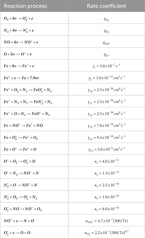
Table 1. Reaction processes and rate coefficients for molecular ions and metallic species as used into MIRE.

Finally, by assuming charge neutrality condition for the ionospheric plasma (${\left[\mathrm{N}\right.}_{\mathrm{e}}]={\displaystyle {\sum }_{\mathrm{i}}}{\mathrm{N}}_{\mathrm{i}}$), we can simulate from MIRE the electron density (N_e) profile (Eq. 11) in a space-time of approximately 0.2 km height every 2 min between 00 and 24 UT. This allows to extract the height variation of the simulated ILs (Carrasco et al., 2007; Resende et al., 2017; Conceição-Santos et al., 2019):

${\mathit{N}}_{\mathit{e}}=\left[{\mathit{O}}_{\mathbf{2}}^{+}\right]+\left[{\mathit{N}\mathit{O}}^{+}\right]+\left[{\mathit{O}}^{+}\right]+\left[{\mathit{N}}_{\mathbf{2}}^{+}\right]+\left[{\mathit{F}\mathit{e}}^{+}\right]+\left[{\mathit{M}\mathit{g}}^{+}\right].(11)$

3 Results and discussion

3.1 Daily and seasonal distribution of the intermediate E-F layers

Figures 2, 3 show mass plots of the virtual height (h'IL) and the top frequency (ftIL) parameters of the ILs observed from ionosonde measurements at SJC and PAL stations, respectively. Figure 2 shows the hourly (in Universal Time) and seasonal variation of h'IL (red dots) and ftIL (blue dots) as observed for the station of SJC during the equinoxes (top panels), the winter solstice (middle panels), and the summer solstice (bottom panels) months. Figure 3 was constructed similarly to Figure 2 but denotes the hourly and seasonal variation of h'IL and ftIL over the PAL station. The thick black lines in these plots represent the mean values, whereas the red (blue) dots denote the daily measurements of the h'IL (ftIL) parameters. The numbers at the top within the panels of both figures indicate the number of days on which ILs were observed. The ILs were observed on more than 90% of available data days in SJC and more than 80% in PAL.

Figure 2

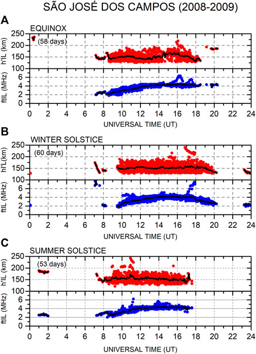
Figure 2. Mass plots of the diurnal virtual height (h’IL) and the top frequency (ftIL) parameters of the ILs obtained from the ionograms at SJC during the equinox (A), winter (B), and summer (C) months of 2008–2009.

Figure 3

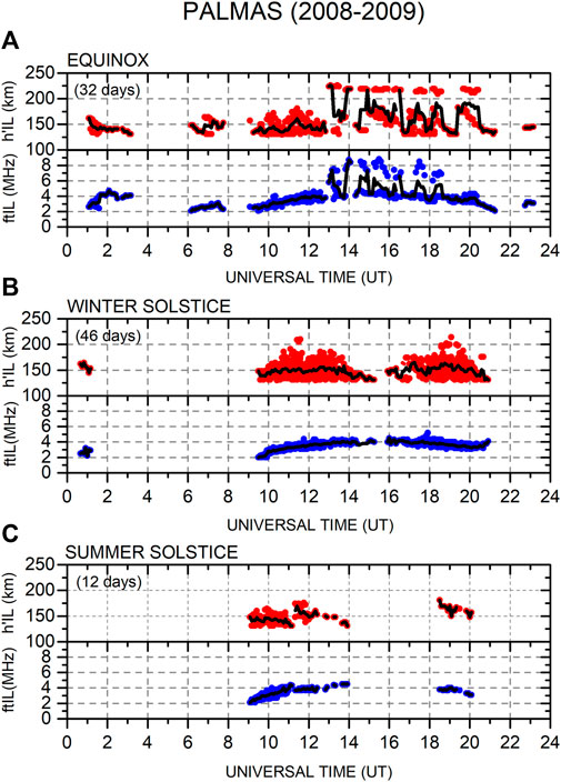
Figure 3. Mass plots of the diurnal virtual height (h’IL) and the top frequency (ftIL) parameters of the ILs obtained from the ionograms at PAL during the equinox (A), winter (B), and summer (C) months of 2008–2009.

It is clearly noticed from Figures 2, 3 that the ILs are observed predominantly during the daytime, that is, between 09 UT (06 LT) and 21 UT (18 LT). This feature of the ILs was also reported in previous studies (e.g., Dos Santos et al., 2019). On the other hand, during the nighttime, ILs events were rare phenomena that predominantly occurred before local midnight (03 UT) over both stations. For example, Figure 2 shows that over SJC, the ILs were observed during a short period between around 00–01 UT (21–22 LT) during the equinoxes, between around 23–24 UT (20–21 LT) during winter solstice, and between around 01–02 UT (22–23 LT) during summer solstice. Whereas in PAL, the nighttime observations of ILs occurred during the equinoxes at ∼23 UT (20 LT) and between around 01–03 UT (22–24 LT), and during the winter solstice months at ∼01 UT (22 LT). During the summer, nocturnal IL was not registered over PAL. In the longitudinal sectors of India and Taiwan, the formation of ILs during the nighttime period was also considered a rare event (Lee et al., 2003; Niranjan et al., 2010; Mridula and Pant, 2022). It is not shown in the plots of Figures 2, 3, but the daily occurrence of ILs during the equinoxes peaks at around 11 UT (08 LT) with values of ∼50% at SJC and ∼20% at PAL. During the winter solstice, the occurrence of ILs peaks between around 11–12 UT (08–09 LT) with values of ∼75% at SJC and ∼42% at PAL, whereas during the summer solstice, it peaks at around 14 UT (11 LT) in SJC with a rate of ∼38%, and at around 10 UT (07 LT) in PAL with a rate of ∼50%. Therefore, as noted from these results, the occurrence rates are higher during morning hours when the ILs are developing and evolving in the ionosphere. Larger occurrence probability of ILs during morning hours was also reported by Lee et al. (2003) for the low-latitude Taiwanese sector. Figures 2, 3 also reveal that the height variability of the ILs ranges mostly between around 130–190 km for all seasonal periods, with maximum mean heights of formation attaining values of ∼240 km at SJC and ∼225 km at PAL during equinoxes. The highest average top frequencies of the ILs (ftIL) over SJC were ∼4.5 MHz during the equinoxes and summer months, and ∼4.0 MHz in the winter solstice. Over PAL, these values were ∼4.5 MHz in summer and winter. However, during the equinoxes in PAL, the average values of ftIL were highly variable between around 4–8 MHz. These maximum values of ftIL were observed above the stations of SJC and PAL close to the local noon (14–16 UT). Niranjan et al. (2010) and Mridula and Pant (2022) reported maximum mean values of critical frequencies of ILs ranging from ∼3.5 to 5.0 MHz around noontime, while Lee et al. (2003) reported monthly mean values of critical frequencies above 6 MHz.

In addition to the nocturnal ionospheric layers (ILs), we also observed the presence of atypical IL behavior during the analysis of ionograms. Specifically, we observed instances of two simultaneous ILs forming at distinct altitudes, as well as ILs exhibiting upward motion within a short time frame. It is important to note that these unusual IL occurrences fall outside the scope of our current investigation (e.g., Dos Santos et al., 2019). The predominant IL signatures, commonly observed at both SJC and PAL sites, entail daytime IL formation through detachment from the F layer base, followed by a subsequent downward motion into the E region. In this study, we analyze the predominant ILs for a better understanding of the underlying factors influencing their dynamics at altitudes below 140 km. We aim to investigate whether any prevailing neutral wind direction and tidal pattern are controlling the descent of ILs. Thus, depending on the month of observations, we also analyze whether there is any seasonal pattern influencing the variation of ILs above the stations.

3.2 Simulated neutral winds

This section presents the results of the wind amplitudes computed from the meteor radars data and used as input into MIRE. Wind measurements were available for the station of Cachoeira Paulista (as representative of the winds over SJC) during October 2008, whereas for the station of São João do Cariri (as representative of the winds over PAL) during April 2009 and June 2009. The tidal oscillations for the zonal and meridional wind components were simulated by MIRE for both stations.

Figure 4 shows contour plots of the wind amplitudes (color scales) in height versus Universal Time (UT) during October 2008 at Cachoeira Paulista. The diurnal (D) tide for the meridional and zonal wind components is shown in the top panels, the semidiurnal (S) tide for the meridional and zonal winds is shown in the middle panels, and the contributions of both the diurnal and semidiurnal (D+S) tides for the meridional and zonal winds are shown in the bottom panels. The panels in Figures 5A, B are like Figure 4 but denote the tidal modes and wind amplitudes for the meridional wind and zonal wind, respectively, during April 2009 and June 2009 at São João do Cariri. The isolines with 0 m.s⁻¹ in Figures 4, 5 indicate the shearing in the neutral winds, which tend to oscillate when both diurnal and semidiurnal tides are simulated for the meridional and zonal wind components.

Figure 4

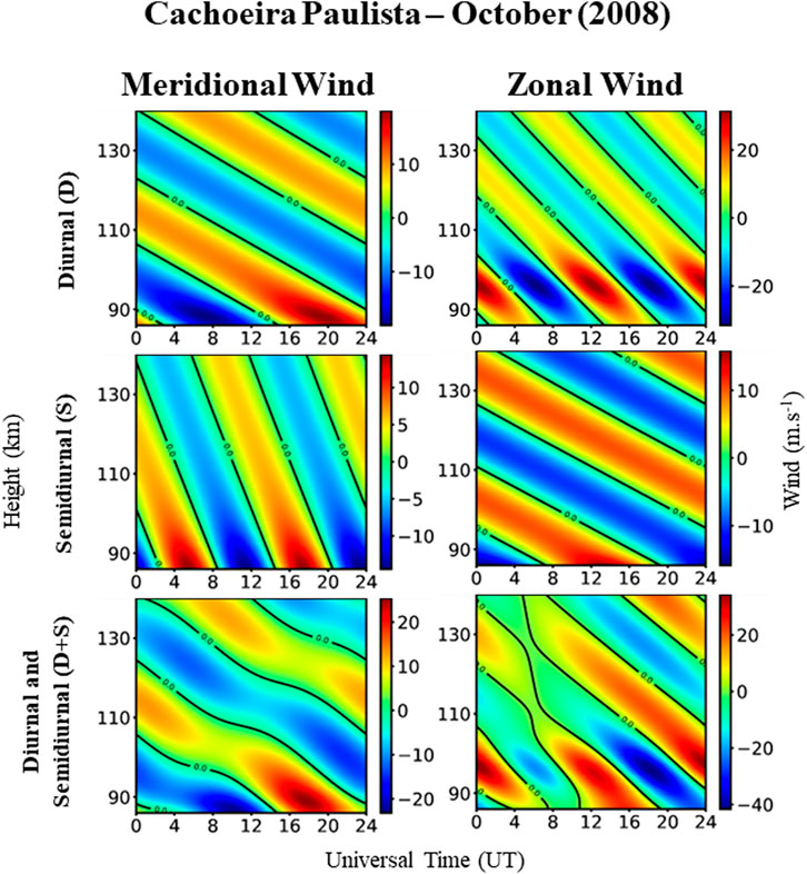
Figure 4. Height-time maps of the diurnal (D) tide (top panels), semidiurnal (S) tide (middle panels), and both diurnal and semidiurnal (D+S) tides (bottom panels) for the meridional (A) and zonal (B) winds, as simulated by MIRE for the station of Cachoeira Paulista during October of 2008.

Figure 5

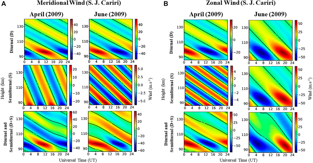
Figure 5. Height-time maps of the diurnal (D) tide (top panels), semidiurnal (S) tide (middle panels), and both diurnal and semidiurnal (D+S) tides (bottom panels) for the meridional wind component (A) and the zonal wind component (B) during April (2009), and during June (2009).

In the equinoctial month of October 2008 at Cachoeira Paulista, the results indicate that the maximum amplitude of the zonal wind is greater (by approximately ∼10 m/s) than the amplitude for the meridional wind when only the diurnal tide is considered in the simulations. On the other hand, when the semidiurnal tide is considered (S and D+S), the maximum amplitudes of the meridional and zonal winds do not differ significantly, except for the vertical profile of both winds that undergo changes. For the São João do Cariri station, it is evident during the equinoctial month of April 2009 that the maximum amplitude of the meridional wind is greater than the amplitude of the zonal wind in all cases (D, S, and D+S). Conversely, during the winter (June 2009) at São João do Cariri, the highest amplitudes are observed in the zonal component for all cases (D, S, and D+S). The results shown here for October 2008 at Cachoeira Paulista and June 2009 for São João do Cariri agree with previous results for altitudes below 140 km reported in the Brazilian sector by Resende et al. (2017). On the other hand, in April 2009, a greater amplitude of meridional wind compared to zonal wind may indicate a possible modification in the seasonal wind pattern over the latitude region near São João do Cariri, thereby affecting the dynamics of the ILs. Figure 5 also reveals that the most significant differences in São João do Cariri occurred when only the semidiurnal tide was considered in the simulations, where in the month of April 2009, the maximum amplitude of the meridional wind was approximately 5 times larger than that of the zonal wind, while in the month of June 2009 the maximum amplitude of the zonal wind was approximately ∼10 times larger than that of the meridional component.

3.3 Comparison between ionosonde data and MIRE simulations

In this section, we present a comparison between the results of height variability of the IL as simulated by MIRE at altitudes below 140 km and the observed values of h'IL. The simulations considered the effects of both meridional and zonal neutral winds, as well as the combined effects of diurnal and semidiurnal tidal periodicities. Here, we aim to analyze 3 months of collected data and compare it with simulation results to determine the prevailing wind direction, which may influence the downward motion of the ILs in altitudes below 140 km.

The panels in Figure 6 show mass plots of the IL virtual height (h'IL) variability (greyish dots) as a function of UT, as observed at SJC (Figure 6A) during October 2008, and at PAL during April (Figure 6B) and June (Figure 6C) of 2009, respectively from upper to lower panels. These months were chosen due to the availability of meteor radar data at the observatories of Cachoeira Paulista (October 2008) and São João do Cariri (April and June 2009). The lines with black circles in the plots denote the monthly mean variations of the measured h'IL. Fitted linear curves (solid black lines) are also shown in the plots to indicate the times when the Rate of Descent (R_D) of the ILs were estimated for each month from observational data, and the associated mean height of the ILs (h'IL_M) during their descending motion. The ILs height variability during each month as simulated by MIRE and considering the combined effects of the diurnal and semidiurnal tidal periodicities (D+S) are shown in the plots for the zonal (blue dots), meridional (red dots), and both the zonal and meridional (olive dots) wind components. The values of R_D and h'IL_M when calculated from the simulations are also indicated within the layer plots. The dash dot line in magenta at 140 km denotes the upper limit of the MIRE model, below which simulations were conducted to investigate the descent phase of ILs.

Figure 6

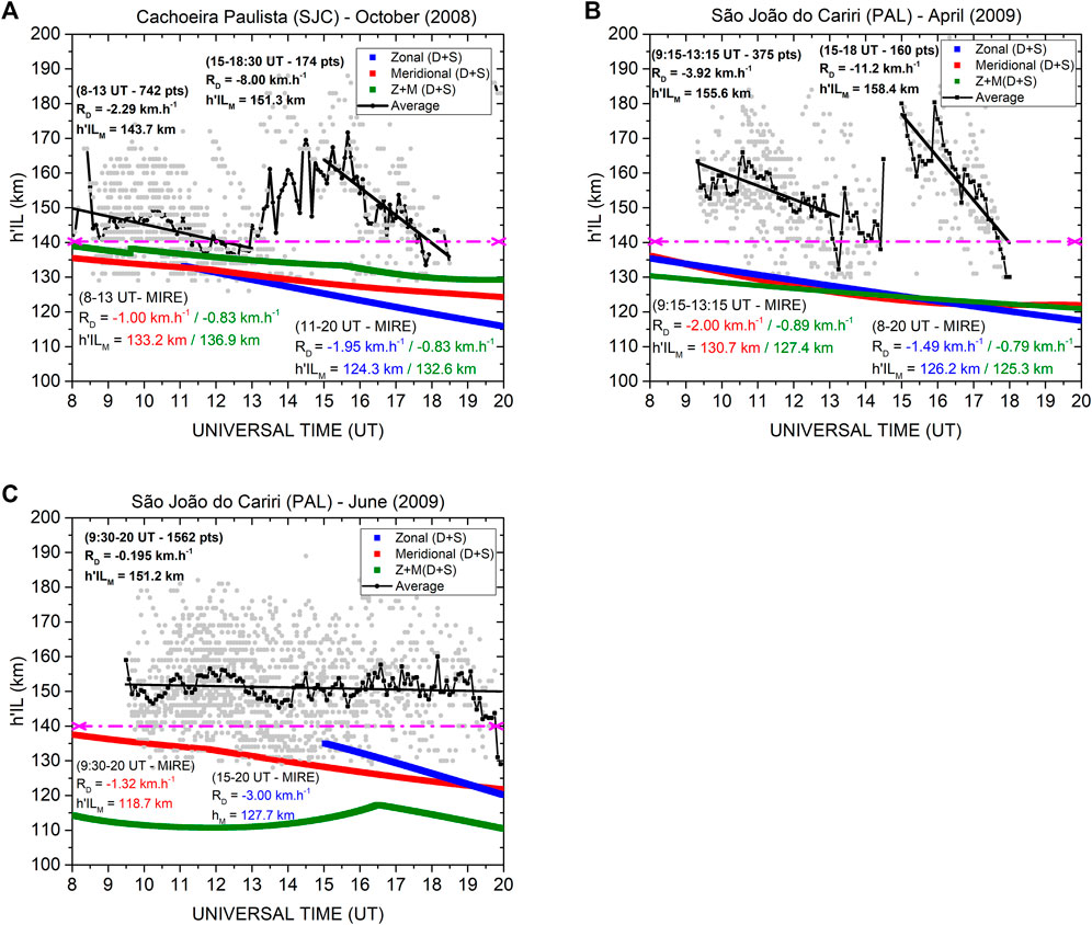
Figure 6. Mass plots of the IL virtual height (h’IL) observed during daytime in October 2008 at SJC (A), April 2009 at PAL (B), and June 2009 at PAL (C). The linear fit of the mass plots is shown as solid black lines during specific times for each month. The solid curves with black circles denote the monthly mean variations of h’IL. The blue (red) lines denote the ILs height variability as simulated by MIRE considering zonal (meridional) neutral winds and both the diurnal and semidiurnal (D+S) tidal periodicities. The olive lines denote the ILs height variability as simulated by MIRE considering both the zonal and meridional wind components (Z+M) and the diurnal and semidiurnal (D+S) tidal periodicities. The dash dot line in magenta at 140 km denotes the upper limit of the MIRE model.

In October 2008 at SJC, it was noted from Figure 6A (top panel) that the ILs were mostly observed between about 08–19 UT (05–16 LT). For this month, which is in the equinoctial period, the results reveal that the ILs are initially formed around sunrise and the first morning hours at heights from 130 to 170 km. Then, the ILs tend to have a descending motion until around 13 UT (10 LT) with a rate (R_D) of −2.29 km.h⁻¹. When analyzing the ftIL parameter (proportional to the electron density of the IL) in the Equinox plot of Figure 2, it is evident that the morning downward motion of the ILs is associated with increases in the density of the ILs. As metallic ions have a slower recombination rate compared to molecular ions, such an increase in density may suggest that neutral winds are populating the region with metallic ions. The value of h'IL_M between 08 and 13 UT was 143.7 km. At around 13 UT, the ILs at lower heights tend to disappear, and new ILs also begin to form at altitudes that may attain 190 km. In fact, the enhancement in the mean height values of the h'IL observed at SJC around noon time, between about 13 and 16 UT (10–13 LT), is associated with the formation of ILs at higher altitudes (150–190 km). Although the ILs are still formed, after 16 UT most of them tend to descend to lower heights until disappear before 19 UT (16 LT). The R_D of the ILs formed after 13 UT was calculated for the time interval from 15 UT to 18:30 UT and presented large values of −8.00 km.h⁻¹ with h'IL_M exceeding 150 km. However, the most important at this point is to check what the results of the MIRE simulations reveal to us. For example, the red, blue, and olive lines in Figure 6A represent the IL height variability simulated by MIRE, considering respectively, the meridional wind component, the zonal wind component, and both the meridional and zonal (Z+M) wind components. We considered both the diurnal and semidiurnal (D+S) tidal oscillations for each wind component in the simulations. According to MIRE simulations, the shearing in the zonal wind component was able of generating a layer after 11 UT (08 LT) with a R_D of −1.95 km.h⁻¹ until 20 UT (17 LT) and h'IL_M of 124.3 km. The meridional wind component in turn generates a layer over 135 km at 08 UT, with a downward movement of −1.00 km.h⁻¹ until 13 UT. The R_D for the meridional wind component was calculated between 08 and 13 UT for comparison with the h'IL height variability obtained from ionosonde measurements at SJC. However, when both the zonal and meridional wind components were considered in the simulation, a higher layer was formed with h'IL_M of 136.9 km between 8–13 UT, and 132.6 km between 11–20 UT. On the other hand, the average values of R_D were lower than the case of separated wind components, with values of −0.83 km.h⁻¹.

It is noticed from Figure 6A that the values of h'IL_M between 08 and 13 UT due to the combined effect of zonal and meridional winds, and the meridional wind alone, are comparable with the observed values of h'IL below 140 km (greyish dots), while the R_D from simulation results is lower than the observed R_D by ∼ from −1.3 to −1.5 km.h⁻¹. Furthermore, within the model coverage height range the layer descending from 135 to 125 km (meridional) and from 139 to 129 (Z+M) between 08 and 20 UT agrees with the observed h'IL (down to 140 km). For the zonal wind, the agreement between modeling and observation appears to be better between 11 and 13 UT, when analyzing the R_D values and the layer descent height range (133–129 km). In fact, for this month of October 2008 the simulation results suggest that the interaction between the zonal and meridional winds was important to generate ILs at heights of ∼130–140 km. According to Osterman et al. (1995), such interaction is expected to affect the size and shape of the ILs, with the meridional wind being effective in descending the layer only up to around 125 km (in agreement with our simulations). We may also deduce from observations (black lines) that between 13 and 16 UT (around noon) the ionization increases, and the molecular ions are possibly converging vertically to form ILs at higher altitudes as result of the shearing in the horizontal neutral winds. At around noon, the MIRE model was not able to describe the change in IL behavior, both for the zonal and meridional wind components. After 15 UT the observed ILs descended with a high rate (−8.00 km.h⁻¹), while the simulations provided R_D values from ∼−0.83 to −2.00 km.h⁻¹. Additionally, it is well known that the meridional wind dominates in forming ILs at higher altitudes and subsequently causes their descent at rates between 5 and 8.5 km.h⁻¹ (Osterman et al., 1995; Szuszczewicz et al., 1995), which agrees with the R_D values obtained here from measurements between 15 and 18:30 UT. Moreover, according to Williams (1996), descent rates ranging from 7 to 11 km.h⁻¹ are characteristic velocities of semidiurnal tidal modes, which also tend to dominate at higher altitudes. Therefore, it is noticeable from the simulation results for the month of October 2008 that the combined effect of the zonal and meridional components of the wind played an important role in the descending motion of ILs below 140 km. Moreover, semidiurnal tide is expected to be dominating above 140 km, while within the height range of 125–140 km, MIRE simulations indicate that the diurnal tide also becomes significantly influential in shaping the periodicities of ILs. It is important to mention that when the diurnal and semidiurnal tidal modes were separately considered in the zonal and meridional winds (not depicted in the plots), the simulation results did not show the presence of layers during daytime hours. Alternatively, when layers were formed, they occurred at lower altitudes, exhibiting larger discrepancies with the observations.

For April 2009 at PAL, it is noted from Figure 6B (middle panel) that the ILs were mainly observed between about 09–18 UT (06–15 LT) at a height range of 130–180 km. For this month, which is also in the equinoctial period, the behavior of ILs is like what was previously observed in October 2008 regarding SJC. The daily behavior of the ILs reveals that the layers initially formed shortly after dawn above 140 km. These layers formed early in the morning begin to descend, while other layers tend to form at progressively higher altitudes until around 11 UT at a maximum height of ∼190 km. From 09:15 to 13:15 UT (06:15–10:15 LT) the ILs descended at a rate of −3.92 km.h⁻¹ and with h'IL_M of 155.6 km. As layers formed during the morning hours descend to lower altitudes, they tend to dissipate until around 14 UT (11 LT). Then, new layers form between 15 and 17 UT (12–14 LT) at heights from 160 to 200 km. As PAL station is located closer to the magnetic equator, the presence of ILs at higher altitudes is expected to be higher when compared to lower-latitude regions, owing to the configuration of magnetic field lines and more efficient ionization processes at these regions. After 15 UT the observed ILs descended with a high rate (−11.2 km.h⁻¹) and presented h'IL_M of 158.4 km. The high values of R_D of the ILs observed over PAL after local noon time are similar to what was previously observed for October 2008 at SJC, which suggests that the role of meridional winds and semidiurnal tidal oscillations are dominant at higher altitudes. Santos et al. (2020) have also reported similar observations in the Brazilian sector. However, concerning the results of the MIRE model, three noteworthy aspects from the simulations are worth mentioning. Firstly, it is observed that both the zonal and meridional components of the winds seem to be interacting with each other and forming layers below 140 km throughout the entire analyzed time range (08–20 UT). Secondly, by analyzing separately the effects of the zonal and meridional winds it is noticed that the altitude range of layer formation closely overlap between 09 and 18 UT (06–15 LT). Finally, it is noted that, as the layers were formed at higher altitudes over PAL, the modeled h'IL values consistently remained below the observed minimum values of h'IL. Furthermore, the R_D values obtained from ionosonde observations between 09:15 and 13:15 UT were nearly twice those obtained through the model considering only the meridional wind, and four times higher than the R_D value for the combined Z+M modeling result. Descent rates of 3–4 km.h⁻¹ have also been associated with semidiurnal tides (Nygren et al., 1990; Niranjan et al., 2010). Such discrepancies found in the R_D between observations and model might be associated to the fact that, interactions between tides with other types of atmospheric waves, such as gravity or planetary waves, have not been considered into the model. Additionally, a potentially undetected weaker tidal mode could be contributing to the impact on IL dynamics associated with tidal winds (e.g., Haldoupis and Pancheva, 2006; Fontes et al., 2023). Analyzing the model results, we can state that for April 2009 in PAL, the roles of both zonal and meridional winds seem to be equally important and are influencing the dynamics of ILs below 140 km, especially during the period between 11 and 13:30 UT (08–10:30 LT) when the modeled values of h'IL are closer to the observed heights. It is also important to highlight here that the model responded better when both diurnal and semidiurnal (D+S) tidal periodicities were considered for the combined and separated components of the winds.

In June 2009 at PAL, the variability of the ILs was quite different from that observed in April. This is probably associated in part with the fact that June is typically a month of the winter seasonal period. It is clear from Figure 6C (bottom panel) that the ILs appear to have formed in a more dispersed manner throughout the months between 130 and 180 km in altitude. Additionally, from the curve of the mean values of the height h'IL, it is observed that the layers tend to oscillate throughout the day, exhibiting peaks and valleys with periods of 30–90 min. This indicates that other local modulations with time scales smaller than the diurnal and semidiurnal tidal modes may be playing a role in the IL formation process. Similar behavior was reported by Earle et al. (2000) from ILs observations at Arecibo. More recently, Santos et al. (2020) also observed h'IL oscillations over the equatorial site of São Luís, Brazil, and suggested that gravity waves-induced electric fields might be causing such oscillations. Figure 6C also shows that the ILs began to form around 09:30 UT (06:30 LT) and tend to descend slowly to lower altitudes. Throughout the month of June, the R_D was around 0.2 km.h⁻¹, lower than the values observed in the other months analyzed here. However, the h'IL_M was 151.2 km, similar to the values observed in October 2008 and April 2009 for the SJC and PAL stations, respectively. Most of the ILs were formed between 09:30–15 UT, with the number of layers tending to decrease after noon, and by around 20 UT (17 LT) the ILs ceased completely due to their descent to lower altitudes, possibly because of their gradual merging with the Es layers (Mathews and Bekeny, 1979; Niranjan et al., 2010; Shaikh et al., 2024). The downward movement of ILs after local midday, accompanied by a decrease in electron density (as inferred in Figure 3 for ftIL during winter), may suggest that the zonal wind is becoming more effective in the plasma transport process (e.g., Carter and Forbes, 1999). Indeed, the simulation results using MIRE indicate that down to 140 km the zonal winds began to play a role in the downward movement of the ILs just after noon. Although the R_D of the modeled layer for zonal winds is much higher than observed, the values of the modeled h'IL are close to the observed heights, at least until around 17 UT (14 LT). On the other hand, the model results reveal that the meridional wind was active throughout the entire time interval in which the ILs were observed, especially during the morning period (before noon) when it is dominant. However, when both wind components were combined (Z+M), the model generated layers at much lower altitudes and their dynamics were visibly modified. Thus, it becomes evident from modeling results, that in June 2009 both the meridional and zonal winds are not interacting with each other to control the dynamics of the ILs down to 140 km. Therefore, the vertical shears of meridional wind (D+S) are possibly controlling the descending and even the formation of ILs during the morning hours in June over PAL, while the role of the zonal wind (D+S) becomes relevant after midday for altitudes below 140 km.

4 Summary and conclusion

This study focuses on the observation and modeling of the downward motion of Intermediate E-F Layers (ILs) formed at low latitudes in the Brazilian sector. Observations were conducted during the months of October and December of 2008, as well as in January, April, June, and July of 2009. Initially, we analyzed digital ionosonde data recorded by the observatories of São José dos Campos (SJC) and Palmas (PAL) to investigate the seasonal variation of the virtual height (h'IL) and top frequency (ftIL) parameters of the ILs. The predominant type of ILs observed in the ionograms of SJC and PAL originated from the detachment of the F layer base, followed by subsequent downward motion. The daily occurrence of ILs peaked during the morning hours (before 11 LT) at both SJC and PAL for all seasonal periods. Except during the summer solstice months, the occurrence of ILs was higher in SJC than in PAL during winter and equinoxes. Throughout all seasonal periods analyzed in this work, the daily height variability of the ILs at SJC and PAL mostly ranged between 130 and 190 km, with the highest values of ftIL observed between 4 and 5 MHz around local noon at both stations.

In terms of modeling, diurnal and semidiurnal tides for zonal and meridional winds, as inferred from meteor radar data, were used as input parameters for the MIRE model. The purpose of these simulations was to analyze the prevailing neutral wind component and tidal periodicities influencing the ILs’ altitude descent at E region heights (below 140 km). Simulations were conducted for October 2008 (representing SJC), and April and June 2009 (representing PAL). The MIRE model was capable to reproduce the shearing in neutral winds for both diurnal and semidiurnal tides, revealing distinct oscillations in the shearing profiles when considering both tidal periodicities. The amplitude of the winds varied, depending on the month analyzed and the type of tidal periodicity considered in the simulations.

In October 2008 for SJC and April 2009 for PAL, observations showed a similar behavior of ILs. These layers were observed to form around dawn at altitudes ranging from 130 to 180 km, subsequently descending (accompanied by increases in ftIL) until late morning. New layers begin to emerge around midday at altitudes above 160 km. After midday, these newly formed ILs descended at a rate (R_D) approximately three times greater than that observed in the morning hours. In both months, the signature of the ILs on the ionograms tended to fade between 18–19 UT (15–16 LT) due to the descent of the ILs to lower altitudes and possibly because of their gradual merging with the Es layers present just below (Mathews and Bekeny, 1979; Niranjan et al., 2010; Shaikh et al., 2024). For October 2008 in SJC, the MIRE model revealed that vertical shears in the meridional wind were more effective than shears in the zonal wind in controlling the downward motion of the layers (down from 140 km), a finding also observed in the modeling studies by Wilkinson et al. (1992) and Bishop and Earle (2003). However, a possible interaction between zonal and meridional winds may occur at heights of 129–139 km around 08–20 UT (05–17 LT), contributing to the weakening of the ILs as their size and shape may have been affected, which was also reported by Osterman et al. (1995). Moreover, in the height range of 125–140 km, the simulations revealed that the diurnal and semidiurnal tidal periodicities seemed equally important to the dynamics of the ILs. On the contrary, for April 2009 in PAL, although the modeled values of h'IL were consistently lower than the observed ones, it appeared that diurnal and semidiurnal periodicities in both zonal and meridional winds worked in conjunction to generate and descend the ILs. A general observation from the model for October 2008 in SJC and April 2009 in PAL is that the modeled R_D (below 140 km) was consistently underestimated compared to the values of R_D obtained at higher altitudes from observations. The discrepancies between observed and modeled R_D values might be associated to the fact that, interactions between tides with other types of atmospheric waves have not been considered into the model. Furthermore, an undetected weaker tidal mode might also be adding up to affect the tidal winds, and consequently the IL dynamics.

Finally, in June 2009, the behavior of the ILs over PAL proved to be somewhat different from that observed in the other months analyzed in this study. In addition to a considerably lower decay rate (∼0.2 km/h), the layer exhibited daily oscillations that may be associated with local modulations induced by gravity waves. However, the prospective role of gravity waves in the formation and dynamics of ILs remains a subject requiring further investigation. The simulation results obtained from MIRE indicated that, in June 2009 over PAL, the shearing in the meridional wind with both diurnal and semidiurnal tidal periodicities (D+S) controlled the downward movement of ILs during the morning period. The role of zonal wind vertical shear (D+S) became relevant only after midday, contributing to the downward motion of the layer and causing a reduction in electron density.

Data availability statement

The raw data supporting the conclusion of this article will be made available by the authors, without undue reservation.

Author contributions

MM: Conceptualization, Data curation, Formal Analysis, Funding acquisition, Investigation, Methodology, Project administration, Supervision, Validation, Visualization, Writing–original draft, Writing–review and editing. AS: Conceptualization, Investigation, Methodology, Validation, Visualization, Writing–original draft. AdS: Conceptualization, Funding acquisition, Investigation, Supervision, Writing–review and editing. VP: Data curation, Funding acquisition, Resources, Software, Supervision, Writing–review and editing. LR: Software, Validation, Writing–review and editing. VA: Data curation, Resources, Writing–review and editing. PF: Data curation, Funding acquisition, Project administration, Resources, Writing–review and editing.

Funding

The authors declare that financial support was received for the research, authorship, and/or publication of this article. This research was supported by the Fundação de Amparo à Pesquisa do Estado de São Paulo-FAPESP (grant no. 2022/14815-5), the Conselho Nacional de Desenvolvimento Científico e Tecnológico-CNPq (grant no. 314261/2020-6), and Coordenação de Aperfeiçoamento de Pessoal de Nível Superior-CAPES (grant no. 88887.596362/2020-00).

Acknowledgments

AdS, LR, and VA thank the China–Brazil Joint Laboratory for Space Weather (CBJLSW), National Space Science Center (NSSC), Chinese Academy of Sciences (CAS), for supporting their postdoctoral fellowships. The authors thank Dr. Paulo Batista for providing the meteor radar data and Dr. Alexander Carrasco for authorizing the use of MIRE.

Conflict of interest

The authors declare that the research was conducted in the absence of any commercial or financial relationships that could be construed as a potential conflict of interest.

Publisher’s note

All claims expressed in this article are solely those of the authors and do not necessarily represent those of their affiliated organizations, or those of the publisher, the editors and the reviewers. Any product that may be evaluated in this article, or claim that may be made by its manufacturer, is not guaranteed or endorsed by the publisher.

References

Bailey, G. J., and Sellek, R. (1990). A mathematical model of the Earth’s plasmasphere and its application in a study of He⁺ at L = 3. Ann. Geophys. 8, 171–190.

Google Scholar

Bishop, R. L., and Earle, G. D. (2003). Metallic ion transport associated with midlatitude intermediate layer development. J. Geophys. Res. 108, 1019. doi:10.1029/2002JA009411

CrossRef Full Text | Google Scholar

Carrasco, A. J., Batista, I. S., and Abdu, M. A. (2007). Simulation of the sporadic E layer response to prereversal associated evening vertical electric field enhancement near dip equator. J. Geophys. Res. Space Phys. 112, A06324. doi:10.1029/2006JA012143

CrossRef Full Text | Google Scholar

Carter, L. N., and Forbes, J. M. (1999). Global transport and localized layering of metallic ions in the upper atmospherer. Ann. Geophys. 17, 190–209. doi:10.1007/s00585-999-0190-6

CrossRef Full Text | Google Scholar

Chen, W. M., and Harris, R. D. (1971). An ionospheric E-region nighttime model. J. Atmos. Terr. Phys. 33, 1193–1207. doi:10.1016/0021-9169(71)90107-3

CrossRef Full Text | Google Scholar

Conceição-Santos, F., Muella, M. T. A. H., Resende, L. C. A., Fagundes, P. R., Andrioli, V. F., Batista, P. P., et al. (2020). On the role of tidal winds in the descending of the high type of sporadic layer (Es). Adv. Space Res. 65, 2131–2147. doi:10.1016/j.asr.2019.11.024

CrossRef Full Text | Google Scholar

Conceição-Santos, F., Muella, M. T. A. H., Resende, L. C. A., Fagundes, P. R., Andrioli, V. F., Batista, P. P., et al. (2019). Occurrence and modeling examination of sporadic-E layers in the region of the South America (Atlantic) magnetic anomaly. J. Geophys. Res. Space Phys. 124, 9676–9694. doi:10.1029/2018JA026397

CrossRef Full Text | Google Scholar

Dos Santos, A. M., Batista, I. S., Abdu, M. A., Humberto, J., Sobral, J. H. A., Souza, J. R., et al. (2019). Climatology of intermediate descending layers (or 150km echoes) over the equatorial and low-latitude regions of Brazil during the deep solar minimum of 2009. Ann. Geophys 37, 1005–1024. doi:10.5194/angeo-37-1005-2019

CrossRef Full Text | Google Scholar

Earle, G. D., Bishop, R. L., Collins, S. C., González, S. A., and Sulzer, M. P. (2000). Descending layer variability over Arecibo. J. Geophys. Res. Space Phys. 105, 24951–24961. doi:10.1029/2000JA000029

CrossRef Full Text | Google Scholar

Fontes, P. A., Muella, M. T. D. A. H., Resende, L. C. A., Andrioli, V. F., Fagundes, P. R., Pillat, V. G., et al. (2023). Effects of the terdiurnal tide on the sporadic E (E_s) layer development at low latitudes over the Brazilian sector. Ann. Geophys. 41, 209–224. doi:10.5194/angeo-41-209-2023

CrossRef Full Text | Google Scholar

Fujitaka, K., and Tohmatsu, T. (1973). A tidal theory of the ionospheric intermediate layer. J. Atmos. Terr. Phys. 35, 425–438. doi:10.1016/0021-9169(73)90034-2

CrossRef Full Text | Google Scholar

Haldoupis, C. (2012). Midlatitude sporadic E, A typical paradigm of atmosphere-ionosphere coupling. Space Sci. Rev. 168, 441–461. doi:10.1007/s11214-011-9786-8

CrossRef Full Text | Google Scholar

Haldoupis, C., and Pancheva, D. (2006). Terdiurnal tidelike variability in sporadic E layers. J. Geophys. Res. 111, A07303. doi:10.1029/2005JA011522

CrossRef Full Text | Google Scholar

Kudeki, E., and Fawcett, C. D. (1993). High resolution observations of 150km echoes at Jicamarca. Geophys. Res. Lett. 20, 1987–1990. doi:10.1029/93GL01256

CrossRef Full Text | Google Scholar

Lee, C.-C., Liu, J.-Y., Pan, C.-J., and Hsu, H.-H. (2003). The intermediate layers and associated tidal motions observed by a Digisonde in the equatorial anomaly region. Ann. Geophys. 21, 1039–1045. doi:10.5194/angeo-21-1039-2003

CrossRef Full Text | Google Scholar

Mathews, J. D., and Bekeny, F. S. (1979). Upper atmosphere tides and the vertical motion of ionospheric sporadic layers at Arecibo. J. Geophys. Res. 84, 2743–2750. doi:10.1029/JA084iA06p02743

CrossRef Full Text | Google Scholar

Miller, N. J., Grebowsky, J. M., Hedin, A. E., and Spencer, N. W. (1993). Equatorial ion composition, 140-200 km, based on Atmosphere Explorer E data. J. Geophys. Res. 98, 15685–15692. doi:10.1029/93JA01147

CrossRef Full Text | Google Scholar

Mridula, N., and Pant, T. K. (2022). Occurrence features of intermediate descending layers [IL] over the equatorial location of Thiruvananthapuram. Adv. Space Res. 69, 2102–2110. doi:10.1016/j.asr.2021.12.003

CrossRef Full Text | Google Scholar

Niranjan, K., Srivani, B., and Naidu, V. V. S. (2010). Daytime descending intermediate layers observed over a sub-tropical Indian station Waltair during low-solar activity period. Ann. Geophys. 28, 807–815. doi:10.5194/angeo-28-807-2010

CrossRef Full Text | Google Scholar

Nygren, T., Lanchester, B. S., Huukskonen, A., Jalonen, L., Turunen, T., Rishbeth, H., et al. (1990). Interference of tidal and gravity waves in the ionosphere and an associated sporadic-E layer. J. Atmos. Terr. Phys. 52, 609–615. doi:10.1016/0021-9169(90)90056-S

CrossRef Full Text | Google Scholar

Oikonomou, C., Leontiou, T., Haralambous, H., Gulyaeva, T. L., and Panchenko, V. A. (2023). Occurrence features of intermediate descending layer and Sporadic E observed over the higher mid-latitude ionospheric station of Moscow. Earth Planets Space 75, 39. doi:10.1186/s40623-023-01796-6

CrossRef Full Text | Google Scholar

Osterman, G. B., Heelis, R. A., and Bailey, G. J. (1995). Effects of zonal winds and metallic ions on the behavior of intermediate layers. J. Geophys. Res. 100, 7829–7838. doi:10.1029/94JA03241

CrossRef Full Text | Google Scholar

Resende, L. C. A., Batista, I. S., Denardini, C. M., Batista, P. P., Carrasco, A. J., Andrioli, V. F., et al. (2017). Simulations of blanketing sporadic E-layer over the Brazilian sector driven by tidal winds. J. Atmos. Solar-Terr. Phys. 154, 104–114. doi:10.1016/j.jastp.2016.12.012

CrossRef Full Text | Google Scholar

Resende, L. C. A., Shi, J., Denardini, C. M., Batista, I. S., Picanço, G. A. S., Moro, J., et al. (2021). The impact of the disturbed electric field in the sporadic E (Es) layer development over Brazilian region. J. Geophys. Res. Space Phys. 126, e2020JA028598. doi:10.1029/2020JA028598

CrossRef Full Text | Google Scholar

Rodger, A. S., Fitzgerald, P. H., and Broom, S. M. (1981). The nocturnal intermediate layer over South Georgia. J. Atmos. Sol. Terr. Phys. 43, 1043–1050. doi:10.1016/0021-9169(81)90018-0

CrossRef Full Text | Google Scholar

Rowe, J. F. (1993). A statistical summary of Arecibo nighttime E region observations. J. Geophys. Res. 78, 6811–6817. doi:10.1029/JA078i028p06811

CrossRef Full Text | Google Scholar

Santos, A. M., Batista, I. S., Brum, C. G. M., Sobral, J. H. A., Abdu, M. A., and Souza, J. R. (2021). F region electric field effects on the intermediate layer dynamics during the evening prereversal enhancement at equatorial region over Brazil. J. Geophys. Res. Space Phys. 126, e2020JA028429. doi:10.1029/2020JA028429

CrossRef Full Text | Google Scholar

Santos, A. M., Batista, I. S., Sobral, J. H. A., Brum, C. G. M., Abdu, M. A., and Souza, J. R. (2020). Some differences in the dynamics of the intermediate descending layers observed during periods of maximum and minimum solar flux. J. Geophys. Res. Space Phys. 125, e2019JA027682. doi:10.1029/2019JA027682

CrossRef Full Text | Google Scholar

Santos, A. M., Brum, C. G. M., Batista, I. S., Sobral, J. H. A., Abdu, M. A., and Souza, J. R. (2022). Responses of intermediate layers to geomagnetic activity during the 2009 deep solar minimum over the Brazilian low-latitude sector. Ann. Geophys 40, 259–269. doi:10.5194/angeo-40-259-2022

CrossRef Full Text | Google Scholar

Shaihk, M. M., Abusirdaneh, M. A. K., Halawa, S. S., and Fernini, I. (2024). Characteristics of IDL and Es layers and the impact of increasing solar activity on their descent at the Arabian Peninsula. Adv. Space Res. 73, 2404–2417. doi:10.1016/j.asr.2023.11.051

CrossRef Full Text | Google Scholar

Szuszczewicz, E. P., Roble, R. G., Wilkinson, P. J., and Hanbaba, R. (1995). Coupling mechanisms in the lower ionospheric-thermospheric system and manifestations in the formation and dynamics of intermediate and descending layers. J. Atmos. Sol. Terr. Phys. 57, 1483–1496. doi:10.1016/0021-9169(94)00145-E

CrossRef Full Text | Google Scholar

Watts, J. M., and Brown, J. N. (1994). Some results of sweep-frequency investigation in the low frequency band. J. Geophys. Res. 59, 71–86. doi:10.1029/JZ059i001p00071

CrossRef Full Text | Google Scholar

Wilkinson, P. J., Szuszczewicz, E. P., and Roble, R. G. (1992). Measurements and modelling of intermediate, descending, and sporadic layers in the lower ionosphere: results and implications for global-scale ionospheric-thermospheric studies. Geophys. Res. Lett. 19, 95–98. doi:10.1029/91GL02774

CrossRef Full Text | Google Scholar

Williams, P. J. S. (1996). “Tides, atmospheric gravity waves and traveling disturbances in the ionosphere,” in Modern radio science. Editors H. Kohl, R. Ruster, and K. Schlegel (Germany: European Geophysical Society), 139–180.

Google Scholar