 V. V. Dorovskyy
 V. N. Melnik
 A. I. Brazhenko2
94% of researchers rate our articles as excellent or good
Learn more about the work of our research integrity team to safeguard the quality of each article we publish.
Find out more
ORIGINAL RESEARCH article
Front. Astron. Space Sci., 25 June 2024
Sec. Space Physics
Volume 11 - 2024 | https://doi.org/10.3389/fspas.2024.1403135
This article is part of the Research TopicSolar Radio Bursts and their Applications in Space Weather ForecastingView all 5 articles
Introduction: The properties of the S-bursts observed during the storm on 20–21 June 2022 in frequency band 10–32 MHz by the radio telescope URAN-2 are discussed in this paper. The storm was highly populated with other solar bursts, such as Type III bursts and drift pairs. The occurrence rate of S-bursts was very high reaching 60 bursts per minute. All observed S-bursts were characterized by low fluxes with respect to the background radio emission. Thus special processing methods are used to retrieve spectral properties of the bursts. Some individual “long” S-bursts covered the whole frequency band of the URAN-2 radio telescope from 10 to 32 MHz. Such extended in frequency S-bursts were recorded for the first time. 50 extended S-bursts were selected for the further analysis.
Methods: The S-bursts dynamic spectra with time-frequency resolutions of 100 ms and 4 kHz as well as single-frequency profiles were used in the analysis. Due to low S-bursts intensities the drift rates were estimated from the time-differentiated dynamic spectra, highlighting the tracks of the bursts maxima. Polarization dynamic spectra were used for measuring the degree and sense of the S-bursts circular polarization. Individual S-bursts tracks were used for instant coronal inhomogeneities diagnostics. Mean S-bursts parameters retrieved from the statistical processing of the set of 50 bursts were compared with previously obtained ones.
Results: We concluded that by the mean durations, drift rates, frequency extent and the polarization all observed S-bursts could be divided into two separate groups, the “short” and the “long” S-bursts. The power-law index of the drift rate-frequency dependence averaged over all 50 selected bursts was found to be 1.7. It was shown that sources of S-bursts most likely move through the Newkirk corona with the velocities of 0.06–0.08c. The power-law dependence of the “long” S-bursts durations on frequency in frequency band of 12–30 MHz was obtained. Its index equal to −0.61 appeared to be very close to that for Type III bursts. From this dependence the electron velocity dispersion in the beam, responsible for S-bursts generation was calculated. Its value of 0.02 indicates that the beams, responsible for S-bursts generation are almost monoenergetic.
Discussion: It is assumed that non-monotonic appearance of individual S-bursts tracks on the dynamic spectrum reflects density inhomogeneities encountered by the sources on their paths. From the dynamic spectra of such S-bursts the characteristic size and amplitude of these coronal inhomogeneities were detected. From the S-bursts durations and the velocities of their sources the longitudinal sizes of the latter were estimated. It was then shown that the sizes of small-scale coronal inhomogeneities were comparable to those of “long” S-bursts sources. Thus we concluded that individual tracks of the “long” S-bursts can be used for fie diagnostics the coronal plasma at heliocentric heights range from 1.7 to 3.2 Rs, where Rs is the solar radius. On the other hand, these tracks being ensemble-averaged give the information about the long-term large scale properties of the corona.
Solar S-bursts belong to the class of fine structure events of solar sporadic radio emission due to both temporal and frequency narrowness. They were firstly observed mostly in meter band by G.R.A. Ellis with Culgoora radio telescope in 1966–1967 (Ellis, 1969). He distinguished them as a separate type of solar radio bursts mainly by mean values of drift rate (1.9 MHz/s), frequency bandwidth (30 kHz) and duration (0.6 s) averaged in frequency band 25–100 MHz. He informed that S-bursts drift rates were much less than those of normal Type III bursts and slightly larger than drift pairs ones. The bandwidths were much less than those of both Type III bursts and drift pairs. And finally the durations were reported to be considerably less than those of Type IIIs and drift pairs.
Since then, a number of authors have reported observations of solar S-bursts in the meter and decameter bands (McConnell, 1980; McConnell and Ellis, 1981; McConnell, 1982; Zeitsev and Zlotnik, 1986; Barrow et al., 1994; Dorovskyy et al., 2006; Melnik et al., 2010; Morosan et al., 2015; Dorovskyy et al., 2017; Morosan et al., 2017; Clarke et al., 2019; Zhang et al., 2020). Most of them noted that these bursts were comparatively rare and weak events. They can only be episodically observed in years of maximal solar activity. In addition, the extremely low fluxes of these bursts (0.1–50 s.f.u. according to McConnell (1982), where 1 s.f.u. = 10–22 Wm−2Hz−1) required the use of highly sensitive meter and decameter band radio telescopes.
The first S-bursts analysis made by Ellis was continued by D. McConnell one solar cycle later. He observed intense S-bursts storm with Llanherne radio telescope in 1979 in frequency band 30–82 MHz with much better time resolution of 1 ms and good frequency resolution of 10 kHz (McConnell, 1980; 1982). The storm was characterized by very high occurrence rate, reaching 500 S-bursts during 13 min. His observations showed that S-bursts may have much shorter durations than was reported by Ellis (1969), namely, from 5 to 165 ms with a significant number of bursts being shorter than 25 ms at frequencies near 38 MHz. No systematic dependence of the duration on frequency were detected by that time. First attempt to find such dependence was made by Dorovskyy et al. (2017). Authors processed about 1,000 S-bursts in frequency band of 10–32 MHz and found the dependence index to be equal to −1.5.
According to Ellis (1969) and McConnell and Ellis (1981) the instantaneous bandwidth of the observed S-bursts could vary over a rather wide range from 30 up to 200 kHz. The dependence of the bandwidth on frequency also wasn’t obtained. Later Melnik et al. (2010) found that the instantaneous frequency bandwidth of S-bursts linearly increases with frequency. The bandwidth was assumed to be defined by the local magnetic field (Melnik et al., 2010). This allowed to retrieve the magnetic field profile at the heliocentric distances 1.4–2.5 Rs based on the data from joint observations by the LOFAR and the UTR-2 (Clarke et al., 2019).
A fine structure in the form of narrowband and non-drifting in time “fringes” were found in about 1% of all observed S-bursts (McConnell and Ellis, 1981). Bandwidths and frequency separation between neighboring elements were 20–100 kHz. The existence of “fringes” in S-bursts observed at frequencies 10–32 MHz was also confirmed in observations by Dorovskyy et al. (2006, 2017).
As was already mentioned, S-bursts were characterized by relatively small fluxes, which were informed to lie between 0.1 and 50 s.f.u. (Ellis, 1969; McConnell and Ellis, 1981; Dorovskyy et al., 2006; Melnik et al., 2010). Taking into account highest reported fluxes of Type III bursts [106 s.f.u. according to Melnik et al. (2011)], Type II bursts [106 s.f.u. according to Dorovskyy et al. (2015)], Type IV bursts [103 s.f.u. according to Melnik et al. (2008)], drift pairs [103 s.f.u. according to de La Noe and Moller Pedersen (1971)] and spikes [up to 300 s.f.u. according to Melnik et al. (2014)] we may conclude that S-bursts are the only type of solar bursts whose fluxes never exceed 100 s.f.u.
Both Ellis (1969) and McConnell (1982) pointed out that S-bursts were circularly polarized in the sense coinciding with that of accompanying events. Morosan et al. (2015) reported that S-bursts were significantly more polarized than the Type III bursts. In all cases no quantitative estimations were given.
First comparison of the parameters of S-bursts, recorded during different storms spaced in time by different intervals were performed by Dorovskyy et al. (2006) and Melnik et al. (2010) in the frequency band 18–30 MHz. They analyzed S-burst observed in few neighboring days within one storm, as well as in storms which were 2 weeks, a month and a year apart during the maximum of 23-d (twenty third) solar cycle. They found that while main parameters of S-bursts during one individual storm have narrow distributions, their mean values obtained for different storms may differ more significantly. Also they reported that in all cases S-bursts only occurred when the associated active regions were located near the central meridian.
First attempt to detect the size and location of S-bursts sources were done by Morosan et al. (2015) who used the LOFAR tied-array imaging technique. Authors didn’t provide any exact numbers but only stated that the S-bursts sources were smaller than the Type III bursts ones.
Recently Zhang et al. (2020) observed an S-bursts storm with a single HBA beam of the LOFAR core station in frequency band ∼120–180 MHz and traced some individual bursts across the dynamic spectrum. Currently these are the highest frequencies at which S-bursts were observed. Authors discovered that individual S-bursts sometimes manifest non-monotonic wave-like drift on frequency as well as flux modulation along their track. Assuming radiation at fundamental frequency they connected all these effects with coronal plasma density irregularities, which caused variation in the optical depth of the source and hence the intensity modulation.
Plasma emission mechanism is now generally accepted for interpretation of the S-bursts generation. Melnik et al. (2010) proposed a model in which S-bursts are generated due to coalescence of the Langmuir and the fast magnetosonic waves, whose phase and group velocities were equal to the electron beam velocity and all of them being equal to about 0.1c, where c is the speed of light.
The structure of the current article is as follows. The details of the observations as well as general characteristics of the events observed on 20–21 June 2022 are given in Section 2. The arguments in favor of existence of two families of solar S-bursts, namely, the “short” and the “long” ones, are considered in Section 3. In Section 4 the properties of the individual tracks of the “long” S-bursts extended over the frequency range ≥14 MHz are analyzed. The method to detect the FWHM duration of weak S-bursts against the intense background radio emission is demonstrated. The dependences of the drift rates and durations on frequency for each individual S-burst as well as the ensemble-averaged dependences are obtained. In Section 5 the possibilities of using the obtained dependences for fine diagnostics of the coronal plasma at the heights of 1.7–3.2 Rs as well as for electron beams diagnostics are discussed.
Observations of the solar radio emission during the summer months of 2022 were carried out with the URAN-2 radio telescope daily from 5:30 to 18:00 UT with resolutions of 100 ms and 4 kHz in time and frequency respectively. This instrument is the second by the effective area Ukrainian radio telescope after the UTR-2. It operates in frequency band of 8–32 MHz and provides the effective area of 28,000 m2 and the beam size of 3,5 ° × 7 ° at frequency of 20 MHz.
On 20–21 June a two-day long storm of S-bursts was recorded. It was not the first time when such a prolong S-bursts storm occurred. A 4-day storm was analyzed by Melnik et al. (2010). The 2022 storm was characterized by extremely high occurrence rate reaching in average about 60 bursts per minute (Figures 1A, B). Another important characteristic of this storm was the frequency extent of the bursts. The frequency range over which separate S-burst could extend was in average 8 MHz. At the same time a certain amount of individual S-bursts, which could be traced across the whole working frequency band of the URAN-2 instrument were also observed. Such extended and low-frequency S-bursts were recorded for the first time. This made it possible to analyze the drift rate and flux irregularities and hence to estimate coronal plasma inhomogeneities as it was done by Zhang et al. (2020) but higher in the corona and in much wider range of heliocentric heights (1.7–3 Rs).
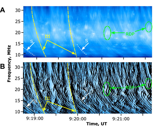
Figure 1. Three-minute fragment of the S-bursts storm on 20–21 June 2022 recorded by URAN-2: (A) normal dynamic spectrum and (B) time-differential dynamic spectrum. Some S-bursts are marked with white arrows, Type III bursts are marked with yellow and reverse drift pairs with green ones.
The distinctive feature of the storm was abnormally high level of the background radio emission in the form of Type III bursts and drift pairs, whose average flux was about 500 s.f.u. Taking into account that S-bursts fluxes never exceed 100 s.f.u. It made almost impossible to accurately analyze the spectral parameters of the bursts, first of all the FWHM duration, in a standard way. Dorovskyy et al. (2017) showed that observations with the UTR-2 radio telescope operating in the interferometric mode allowed to suppress the background radio emission and thus to analyze weak S-bursts. Due to severe damage of the UTR-2 during the war this method could not be used. To solve this difficulty some additional techniques were used. To get correct FWHM duration we used the fact that the isolated S-burst profile was symmetrical (Melnik et al., 2010). So we proposed to approximate the S-bursts profiles with Gaussian curve. The correctness of Gaussian approximation of S-bursts profile and the method of detection of weak S-bursts durations are considered in Section 4.
To get the drift rate and its dependence on frequency we used a time-differential dynamic spectrum, which clearly highlights the bursts maxima and allows us to trace the drift of the bursts maxima in frequency and time with high accuracy (Figure 1B). This spectrum is obtained by time differentiating of the intensity profiles at each frequency channel of the power dynamic spectrum. The main criterion of S-bursts identification is the characteristic drift rate and appearance of the track in the dynamic spectrum.
No interferometric observations were performed thus we were unable to detect the bursts locations and to associate the observed storm with a certain active region directly. Then we relied on the well-known fact that S-bursts used to occur only when the associated active region was near the central meridian (Melnik et al., 2010). On 20–21 June 2022 there were several active regions on the solar disk (Figure 2). Only two of them produced C-class flares - NOAA 13030 and NOAA 13038. Since AR 13030 was on the limb and AR 13038 was near the meridian it was natural to suppose that the latter was likely responsible for the S-bursts generation.
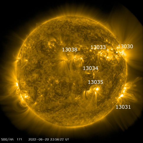
Figure 2. Active regions on the solar disk on 20 June 2022 according to SDO data, taken from https://sdo.gsfc.nasa.gov/data/aiahmi/.
Previous papers on S-bursts showed considerable discrepancies in determining of the S-bursts durations. While Ellis (1969), Melnik et al. (2010) and Clarke et al. (2019) reported that mean S-bursts durations were about 0.5 s, McConnell (1982) informed them to be an order shorter, about 50 ms at frequencies near 38 MHz. Moreover, he pointed out that a number of S-bursts had durations shorter than 25 ms with minimal value reaching 5 ms. For a while this obvious discrepancy appeared to be overlooked by the researchers. During the storm of 20–21 June 2022 the observed S-bursts manifested both the shortest and the longest durations reported before. Detailed analysis of the dynamic spectra shows that the morphology of the shortest and the longest S-bursts is quite different. Figure 3A shows the example of two S-bursts species observed almost simultaneously. It is quite obvious that the “short” S-burst has much shorter duration (no longer than 0.11 s using Gauss fit) and much narrower bandwidth (30 kHz) than the “long” one (1.4 s and 500 kHz respectively). These two bursts have significantly different drift rates. The “short” burst drifts with the rate of about −0.6 MHz/s while the “long” one drifts as only −0.2 MHz/s at frequency of 12 MHz. Moreover, Figure 3B clearly demonstrates that the “short” S-burst is considerably stronger polarized (about 90%) than the “long” one (∼30%). The stair-like appearance of the “short” S-burst in Figure 3A, B is due to the insufficient time resolution in this particular case. Such appearance of the S-burst track may also indicate that the actual duration of this burst is probably less than the time resolution of the equipment being equal to 100 ms.
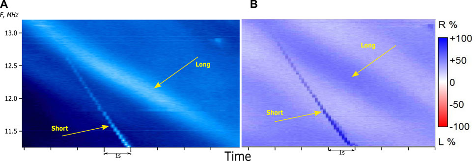
Figure 3. The morphology of the “short” and the “long” S-bursts: (A) amplitude dynamic spectrum and (B) polarization dynamic spectrum.
To determine whether these differences are statistically significant a brief statistical analysis was performed. Since the total amount of the “long” S-bursts covering the whole frequency band of the instrument equaled 50 we selected the same number of the “short” and “long” S-bursts in order to preserve equal statistical samples. To provide equal conditions for both variants of the S-bursts chosen for this analysis we tried to select the bursts observed within as short time interval as possible and approximately at the same frequency. Thus the statistical samples included the short and long S-bursts observed on 21 June between 8:40 and 9:07 UT at frequencies close to 14 MHz. The distributions of their durations and frequency drift rates are shown in Figure 4A, B respectively.
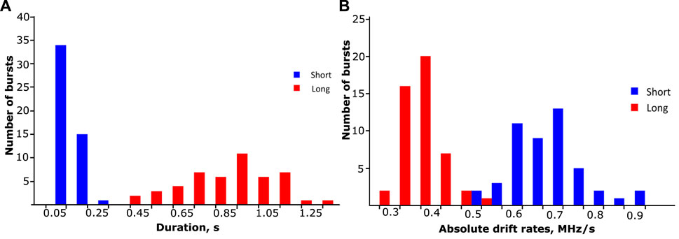
Figure 4. Distributions of the “short” (blue) and “long” (red) S-bursts: (A) by the durations and (B) by the absolute drift rates.
It is clear that each of these two groups of S-bursts have their specific durations and drift rates, which differ significantly. The durations of the “short” S-bursts do not exceed 0.25 s while mean duration of the “long” S-bursts equals 0.8 s. The frequency drift rates of these bursts are −0.7 MHz/s and −0.38 MHz/s, respectively. Moreover, the frequency ranges, over which an individual burst extends are considerably different for the two groups of the observed S-bursts. “Short” S-bursts usually cover the range of 1–2 MHz while the “long” ones extend over the band of around 10 MHz, in rare cases covering the whole frequency band of the radio telescope from 9 to 32 MHz. Mean degrees of circular polarization of the selected sets of S-bursts differ significantly: near 70% for the “short” bursts and about 35% for the “long” ones. The occurrence rate of the latter was much higher. The vast majority of all observed on 20–21 June 2022 S-bursts were the “long” ones.
In addition, we must note that aforementioned assumption that actual durations of the analyzed “short” S-bursts are most likely shorter than the time resolution is illustrated by the detailed durations distribution (Figure 5). Keep in mind that all durations were obtained from the S-bursts profiles approximated with the Gaussian curve.
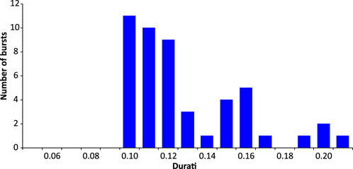
Figure 5. Detailed distribution of the 50 selected “short” S-bursts by their durations.
The obvious trend of the bursts number to increase towards smaller durations and then the abrupt cutoff of the distribution at the duration of 100 ms, which is exactly the time resolution of the equipment, all speak in favor of the assumption that maximum of this distribution lies somewhere below 100 ms and closer to the durations reported by McConnell (1982). All of the above suggests the existence of two separate variants of solar S-bursts: the “short” and the “long” (diffuse) ones.
Previous papers on S-bursts properties (McConnell, 1980; McConnell and Ellis, 1981; McConnell, 1982; Melnik et al., 2010; Morosan et al., 2015; Dorovskyy et al., 2017) were based on study of the mean parameters (e.g., durations and drift rates), which were obtained on the statistical analysis of a large amount of S-bursts, observed at different times during the storm and possibly from different locations of their sources. This technique allowed obtaining general parameters of S-bursts, averaged for periods from several hours up to few days and for different source locations. The dependences derived this way give the information about the long-term and large scale properties of coronal plasma at the corresponding coronal heights, while short-lived and small-scale coronal irregularities are smoothed and washed out. For diagnostics of such small-scale inhomogeneities the analysis of each individual S-burst properties is of great importance. The term small-scale in this context means the scale much smaller than the characteristic scale height of the solar corona.
This idea is not new. The first attempt to analyze the individual S-bursts dynamic spectra was done by Zhang et al. (2020). Authors clearly showed, that the drift rate and flux of each individual S-bursts in some cases may change non-monotonically along the burst track resulting in wave-like appearance of the S-burst on the dynamic spectrum. Sometimes it could even lead to S-bursts segmentation. From the tracks of individual S-bursts authors estimated the sizes and amplitudes of coronal density irregularities to be about 2 ⋅ 10−3Rs and 1 ⋅ 10−3N0, respectively (where Rs is the solar radius and N0 is the local plasma density assuming Newkirk and Gordon (1961) corona model).
At the same time, it should be noted that aforementioned S-bursts were observed at frequencies 120–180 MHz and their frequency extent didn’t exceed 10 MHz. In frames of the Newkirk corona model these frequencies correspond to the heliocentric heights of the emission source of about 1.1–1.2 Rs. Thus an individual S-burst covered the heights range of no more than 0.015 Rs. It is of no doubt that information about such small-scale coronal inhomogeneities higher in the corona is also very important.
The unique feature of the S-bursts storm of 20–21 June 2022 was the existence of the S-bursts which covered almost the entire frequency band of the URAN-2 radio telescope from 9 to 32 MHz. In the Newkirk corona model these boundary frequencies correspond to the heliocentric heights range from 1.7 to 3.2 Rs. Thus it becomes possible to analyze small scale and short-lived coronal inhomogeneities in unprecedentedly wide range of distances. The example of such extended in frequency S-burst is shown in Figure 6. The dynamic spectrum in the figure was 3-point median filtered and then time differentiated.
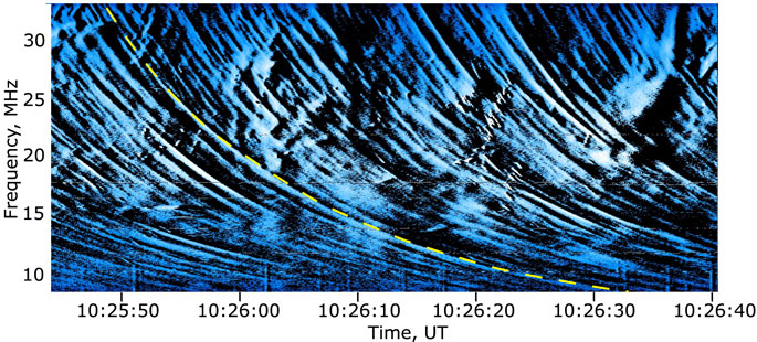
Figure 6. Example of the S-burst extended over the whole frequency band of the URAN-2 (marked with the yellow dashed curve).
During the S-bursts storm on 20–21 June 2022 about 50 bursts extending in frequency wider than 14 MHz were observed. For each of these bursts a set of parameters was obtained at 12 different frequencies from 10 MHz to 32 MHz with a step of 2 MHz. In addition to the drift rates and durations the times and frequencies of the maxima of the bursts were also detected. The latter allowed us to retrieve the individual bursts tracks on the dynamic spectrum. Some “long” S-bursts tracks, which are time-matched at frequency of 30 MHz are shown in Figure 7. The Figure illustrates that for different “long” S-bursts sources it takes from 24.4 to 30.3 s to travel between the 30 MHz and 12 MHz plasma frequency levels. Assuming the Newkirk corona and emission at the fundamental frequency these frequencies correspond to the heliocentric heights of 1.8 Rs and 2.6 Rs, respectively. The observed travel times variation can be attributed to either different source velocities or the non-stationary corona conditions and will be discussed below. In addition to different travel times of the sources some individual tracks of S-bursts manifest non-monotonic appearance on the dynamic spectrum, similar to that described by Zhang et al. (2020). An example of such S-burst is shown in Figure 8A.
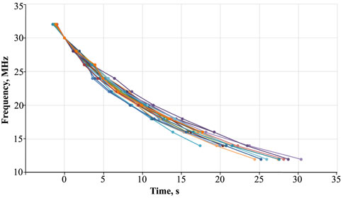
Figure 7. Tracks of the “long” S-bursts time-matched at frequency of 30 MHz.
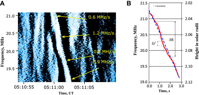
Figure 8. An example of the S-burst with non-monotonic track, observed on 21 June 2022: (A) time-differential spectrum and (B) retrieved track of the burst maximum (red curve) superimposed with expected monotonic track (blue dashed curve). The drift rates at separate frequencies are indicated with arrows.
Figure 8A clearly shows the wave-like oscillation of the drift rate of about ±0.3 MHz/s around the mean value of −0.9 MHz/s. In this particular case the drift rate at a certain frequency was estimated in frequency band of ±200 kHz around each frequency point marked in the figure. The mean frequency drift rate was measured in frequency band of 2 MHz. For each “long” S-burst chosen for the analysis the individual dependences of the drift rates on frequency were obtained. In this case the drift rates were estimated at a set of fixed frequencies spaced by 2 MHz in bandwidths of ±500 kHz around each frequency. Some of 50 individual dependences are shown in Figure 9.
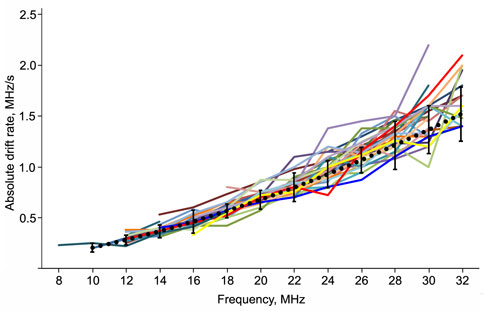
Figure 9. Individual dependences of “long” S-bursts drift rates on frequency.
It is important to note that almost all dependences in Figure 9 are not actually monotonic. At the same time, we didn’t distinguish any correlation between the drift rate and the flux in an individual “long” S-burst, as it was found by Zhang et al. (2020). In this connection we should note that in these two cases we have different plasmas with considerable different absolute densities and the gradients.
To compare the dependences shown in Figure 9 with previously obtained ones we averaged the whole set of curves and approximated the averaged dependence with power-law function in the form of
where
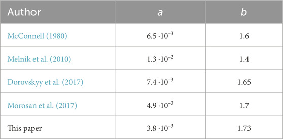
Table 1. The parameters of approximation Eq. 1 obtained by different authors.
One can see that our dependence is in good agreement with the previously obtained ones. All this indicates long-term stability of the parameters of the coronal plasma through which the S-bursts sources move. At the same time, large deviations of individual dependences from each other may be related to the sensitivity of separate sources to small-scale and short-term inhomogeneities of the coronal plasma. In addition, it should be noted that the obtained dependence is in a good agreement with well-known dependence by Alvarez and Haddock (1973) for the Type III bursts, being divided by the factor of 2–4. This indicates that the sources of Type III and S-bursts move through the coronal plasmas with similar mean profiles but with velocities differing by a factor of 2–4.
The duration is one of the distinct features of the S-bursts thus many authors use this parameter in their analysis. Nevertheless, the dependence of the S-bursts durations on frequency has not been obtained until recently (Dorovskyy et al., 2017). This fact is connected with difficulties in S-bursts duration measurement due to their weakness and with absence of the observational data in rather wide frequency band.
As was mentioned earlier, it was impossible to directly measure the FWHM durations of the S-bursts observed in 2022 due to their low fluxes and simultaneously high level of the background radio emission. In such circumstances taking into account symmetrical appearance of an individual S-burst profile we proposed to approximate it with the sum of Gaussian curve and linearly varying background in the form:
where t is the time, I(t) is the flux profile, I0, I1, I2 and τ0 are the parameters of the approximation.
To estimate the correctness of this approximation we selected several individual S-bursts whose profile peaks exceeded the background by a factor of 5–10 and approximated them with Eq. 2. In all cases we got excellent agreement between the experimental profiles and approximations. An example of such approximation is shown in Figure 10.
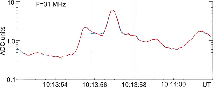
Figure 10. The example of the S-burst profile approximation with the sum of Gaussian curve and linearly varying background. The red curve depicts the original profile, the blue curve shows the approximation with Eq. 2 and the dashed lines delimit the approximation interval.
Thus when approximation parameters of Eq. 2 are found the initial FWHM duration of the S-burst τs can be determined as
This approximation also makes it possible to retrieve the initial flux of the S-burst (parameter I0 in Eq. 2).
From Eq. 2 and Eq. 3 the durations of all 50 selected “long” S-bursts were obtained in the whole frequency band of URAN-2 with a step of 2 MHz. Then we could find the dependence of the S-bursts durations on frequency. This dependence is shown in Figure 11 with the red curve.
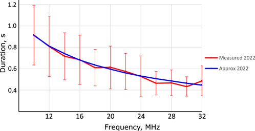
Figure 11. The experimental dependence of the “long” S-bursts duration on frequency (the red curve) and its approximation (the blue curve).
The obtained dependence of the “long” S-bursts durations on frequency was then approximated by the equation:
where τs is the FWHM duration [s] and f is the frequency [MHz]. The approximation Eq. 4 is shown in Figure 11 with the blue curve.
As was mentioned already the index of the drift rate dependence on frequency obtained for the S-bursts appeared to be close to that found by Alvarez and Haddock (1973) for Type III bursts. At the same time Melnik et al. (2021) showed that these dependences for Type III and IIIb bursts agree well with the empirical dependence derived from the Newkirk and Gordon (1961) corona model if source velocity was about 0.2c. Taking into account aforementioned facts and the estimations of Melnik et al. (2010) that S-bursts sources move 2–4 times slower than Type III bursts sources we suppose that the sources of S-bursts move through the Newkirk corona at the speeds of 0.05–0.1c. In order to additionally test whether the Newkirk corona model is suitable for analyzing S-bursts properties, some simple simulations have been preliminarily performed. First, the S-burst tracks were built on the frequency-time plane assuming the source velocity of 0.07c and several corona models, which were the Newkirk (Newkirk and Gordon, 1961), the Baumbach-Allen (Allen, 1947), the Saito (Saito et al., 1977) and the Leblanc (Leblanc et al., 1998) ones. Then from this tracks the dependences of the drift rate on frequency for these corona profiles were built numerically. The obtained data series were then approximated with the power-law Eq. 1. The results are summarized in Table 2.
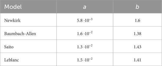
Table 2. Coefficients of Eq. 1 describing the empirical dependences of the drift rate on frequency derived for different corona models.
Table 1, 2 show that the power-law indexes, obtained by different authors and those derived from different corona models deviate by no more than 20%. In particular, Melnik et al. (2010) found this index to range from 1.2 to 1.4 for storms occurred in 2001 and 2002. They attributed this deviation to different corona state during different storms and hence came to the conclusion that the corona may be described by different models at different times. From this we may suppose that the sources of S-bursts observed on 20–21 June 2022 moved through the corona, whose profile was best described by the Newkirk model.
The tracks of individual S-bursts extending over a frequency range from 10 to 32 MHz are the unique diagnostic tool for study the instant corona profiles and the properties of the bursts sources at the heliocentric heights of 1.8–2.6 Rs. The individual tracks indicate rather large variations of the times required by separate sources to travel between the heights corresponding to the local plasma frequencies of 30 and 12 MHz, namely, from 24.4 to 30.3 s. Available set of data doesn’t allow us to separate the contributions of the source velocity and plasma inhomogeneity to the observed variations directly. In the experimental set of data, the fastest S-burst was observed at about 3:53 UT on 21 June 2022 and the slowest one at 5:48 UT on the same day. We tend to consider that large-scale corona properties can’t vary so much during such short time interval and to assume that the travel time variations are connected with different source velocities. Then assuming stationary corona following the Newkirk profile, the above figures mean that the “long” S-bursts sources move at the speeds of 0.06–0.08c. At the same time, it is natural to assume that non-monotonic appearance of the individual tracks is most likely reflects coronal inhomogeneities met by the sources along their paths rather than the velocities variations. The detailed differential dynamic spectrum allows us to determine the amplitude and scale of the electron density inhomogeneity causing the non-monotonic shape of the S-burst track shown in Figure 8A. Figure 8B illustrates how it is done. Here the red curve depicts the track of the maxima of the S-burst shown in Figure 8A across the time-frequency plane. The blue dashed line shows what appearance would have this S-burst track in the case when its source moved through the homogeneous Newkirk corona. The instantaneous frequency difference between the observed and expected frequency (δf) is directly defined by the amplitude of coronal density inhomogeneity. In this particular case it equals about 9 ⋅ 104cm−3 or 1.7% of the background plasma density. At the same time the frequency range which covers the period of quasi-oscillations of the drift rate (and thus the distance between corresponding plasma frequency levels (δR) assuming the Newkirk corona model), is defined by the radial scale of this inhomogeneity. It appears to be about 3 ⋅ 109 cm or 0.04 Rs at heliocentric height of 2 Rs.
Both obtained characteristics are at least by an order of magnitude larger than those found by Zhang et al. (2020) at frequencies near 120 MHz. In our opinion these results do not contradict each other since the characteristic scale of the corona at the level of local plasma frequency of 120 MHz is about an order of magnitude smaller than that corresponding to the frequency of 20 MHz.
It is important to note that the above discussion concerns exclusively the longitudinal sizes of the coronal inhomogeneities. The authors believe that the sensitivity of the burst to the longitudinal coronal inhomogeneities is defined by the relative lengths of the burst exciter and the inhomogeneity. From this point of view all the inhomogeneities with radial sizes less than the length of the electron beam do not manifest themselves in the dynamic spectrum, unlike those whose sizes are comparable or larger than the beam length. The exciter (electron beam) length in its turn is defined by the burst duration and the source velocity. In particular, for the S-bursts, observed on 20–21 June 2022 the source length appeared to be about (1–2) ⋅ 109 cm or not larger than 0.3 Rs. Thus this value delimits the minimal longitudinal scale of the coronal inhomogeneity which can be diagnosed using the observed S-bursts.
Statistical analysis of the S-bursts durations was performed by many authors. Nevertheless, the dependence of this parameter on frequency has not been analyzed. “Long” S-bursts, observed on 20–21 June 2022, which covered a wide range of frequencies, as well as using Gaussian profile fitting, allowed us to obtain reliable dependence of the S-bursts durations on frequency, which is described by Eq. 4. The obtained index of −0.61 is more than 2 times smaller than that found by Dorovskyy et al. (2017), equaled −1.5. In our opinion the discrepancy between two dependences happened due to overestimation of the measured durations of the S-bursts in 2013 at lower frequencies. While the FWHM durations at higher frequencies were measured directly, at lower frequency it was impossible because the bursts appeared to be too weak resulting in overestimation of the durations.
At the same time this index is very close to that of the analogous dependence for Type III bursts, obtained by different authors, which were −2/3 according to Elgaroy and Lyngstad (1972), −0.63 according to Krupar et al. (2020) and −0.59 obtained by Rutkevych and Melnik (2012) from the computer simulations. The only difference between the dependences of Type III and S-burst durations on frequency is the significantly different absolute values, by a factor of 13–16. The closeness of the indexes of these dependences for S-bursts and Type III bursts may indicate similar mechanisms of the bursts duration increase with time.
Currently the plasma emission mechanism is commonly accepted for interpretation of the S-bursts generation (Melnik et al., 2010; Morosan et al., 2015). In this mechanism the exciter is a beam of fast particles having a specific size and moving with a specific speed through the coronal plasma. Rutkevych and Melnik (2012) used a model of spherical beam expanding with the distance from the Sun linearly. They showed that Type III profile may become longer due to increase of the source size mostly along the observer’s line of sight. Later on, Zhang et al. (2019) assumed that the fastest electrons in the beam generated the rise of the burst while the slowest ones were responsible for the burst’s fall generation. The difference between the largest and the smallest velocities is apparently defined by the particles velocity dispersion in the beam. Thus non-zero velocity dispersion would lead to the increase of a burst duration with time. From the dependence of “long” S-bursts durations on frequency we can find the minimal and maximal velocities of their sources. They are vbmin = 2.2 ⋅ 109 cm/s and vbmax = 2.24 ⋅ 109 cm/s. This means that the velocity dispersion in beams responsible for S-bursts generation is Δvb/vb ∼ 2 ⋅ 10–2. One can note that the velocity dispersion of the electrons responsible for the S-bursts generation is rather small. This result can be very important for theoretical interpretation of the S-bursts generation.
The properties of the S-bursts observed during the intense storm on 20–21 June 2022 were discussed.
For the first time individual S-bursts covering the frequency range from 10 to 32 MHz were recorded during the storm. The properties of 50 individual tracks of such bursts observed during 20–21 June 2022 were analyzed. It was shown that individual S-bursts tracks can be used to identify short-term small-scale coronal inhomogeneities. While ensemble-averaged track reflects the long-term and large scale properties of the coronal plasma. From the drift rate dependence on frequency averaged over ensemble of 50 individual dependencies of the long S-bursts observed within 2 days, it was shown that S-burst sources most likely move through the Newkirk corona at velocities of 0.06–0.08c. The closeness of the obtained dependence to those by other authors indicates the long-term and large-scale stability of the corona density profile and the S-bursts sources velocities. It was supposed that non-monotonic appearance of the “long” S-bursts tracks reflects instant small-scale plasma inhomogeneities met by the sources on their paths. From the dynamic spectra these density inhomogeneities were found to have radial size of about 0.04 Rs and the amplitude of ∼1.7%.
The FWHM durations of S-bursts varied in a wide range from 0.1 to 1 s. It was shown that all the observed S-bursts can be divided into two groups mainly by their durations: the “short” S-bursts with the durations less than 100 ms and the “long” ones whose durations were an order of magnitude larger. Moreover, the S-bursts of these two groups differed noticeably by a number of other properties. The “short” S-bursts drifted in frequency twice as fast as the “long” ones at the same frequency. Individual “long” S-bursts extended over rather wide frequency band, sometimes covering the whole band of the URAN-2 instrument, while the “short” ones used to extend over 1–2 MHz. And finally, “short” S-bursts were much stronger circularly polarized than the “long” ones. The obtained duration distributions suggest that “short” S-bursts apparently have durations smaller than measured 100 ms. To make correct durations measurements at frequencies below 30 MHz the observations with time resolution of 5–10 ms are necessary.
The dependence of the “long” S-bursts durations on frequency was experimentally obtained in frequency band 10–32 MHz. The index of this dependence was found to be −0.61 that was very close to that for Type III bursts. We supposed that the bursts durations increased with time due to the electron velocity dispersion in the beam. This dispersion for the case of S-bursts observed on 20–21 June 2022 appeared to be very small and equal Δvb/vb ∼ 10–2. This indicates that the beams responsible for S-bursts generation are almost monoenergetic.
From the obtained values of the S-bursts durations and their sources velocities the longitudinal sizes of the S-bursts sources were estimated. At heliocentric distances 1.7–3 Rs these sizes were about 0.03 Rs. One can see that the source sizes are comparable to the estimated sizes of small-scale coronal inhomogeneities.
At the same time simultaneously observed Type III bursts were rather diffuse and did not exhibit any fine structure. From this we may assume that the sizes of the observed Type III bursts were possibly larger than those of the S-bursts and thus were not sensitive to the small-scale inhomogeneities.
Also for the first time the S-bursts polarization was measured at such low frequencies. The degree of circular polarization of the S-bursts observed on 20–21 June 2022 varied from 30 up to 90%.
The original contributions presented in the study are included in the article/Supplementary material, further inquiries can be directed to the corresponding author.
VD: Conceptualization, Formal Analysis, Investigation, Methodology, Software, Validation, Visualization, Writing–original draft. VM: Project administration, Supervision, Writing–review and editing. AB: Data curation, Resources, Writing–review and editing. AF: Data curation, Software, Writing–review and editing.
The author(s) declare that financial support was received for the research, authorship, and/or publication of this article. The work was funded within the framework of the state budget grants “Complex researches of sporadic radio emission of the Sun during 25 cycle of solar activity” (Radius) (0122U000616) and “Study of the polarization characteristics of decameter radio emission from space sources using the URAN-2 radio telescope” (0118U009760) of the National Academy of Sciences of Ukraine.
The authors express their deep gratitude to the technical staff of the URAN-2 radio telescope for the opportunity to make observations at such a difficult time. VD acknowledges the Europlanet 2024 RI project funded by the European Union’s Horizon 2020 Research and Innovation Programme (Grant agreement No. 871149).
The authors declare that the research was conducted in the absence of any commercial or financial relationships that could be construed as a potential conflict of interest.
All claims expressed in this article are solely those of the authors and do not necessarily represent those of their affiliated organizations, or those of the publisher, the editors and the reviewers. Any product that may be evaluated in this article, or claim that may be made by its manufacturer, is not guaranteed or endorsed by the publisher.
Allen, C. W. (1947). Interpretation of electron densities from corona brightness. Mon. Not. Roy. Astron. Soc. 107, 426–432. doi:10.1093/mnras/107.5-6.426
Alvarez, H., and Haddock, F. T. (1973). Solar wind density model from km-wave type III bursts. Sol. Phys. 29, 197–209. doi:10.1007/BF00153449
Barrow, C. H., Zarka, P., and Aubier, M. G. (1994). Fine structures in solar radio emission at decametre wavelengths. Astron. Astrophys. 286, 597–606.
Clarke, B. P., Morosan, D. E., Gallagher, P. T., Dorovskyy, V. V., Konovalenko, A. A., and Carley, E. P. (2019). Properties and magnetic origins of solar S-bursts. Astron. Astrophys. 622, A204. doi:10.1051/0004-6361/201833939
de La Noe, J., and Moller Pedersen, B. (1971). Relationship between drift pair bursts and decametre type III solar radio emission. Astron. Astrophys. 12, 371.
Dorovskyy, V. V., Melnik, V. N., Konovalenko, A. A., Brazhenko, A., Poedts, S., Rucker, H. O., et al. (2017). “Properties of groups of solar S-bursts in the decameter band,” in Planetary radio emissions VIII. Editors G. Fischer, G. Mann, M. Panchenko, and P. Zarka, 369–378. doi:10.1553/PRE8s369
Dorovskyy, V. V., Melnik, V. N., Konovalenko, A. A., Brazhenko, A. I., Panchenko, M., Poedts, S., et al. (2015). Fine and superfine structure of the decameter-hectometer type II burst on 7 June 2011. Sol. Phys. 290, 2031–2042. doi:10.1007/s11207-015-0725-9
Dorovskyy, V. V., Mel’nik, V. N., Konovalenko, A. A., Rucker, H. O., Abranin, E. P., and Lecacheux, A. (2006). “Observations of Solar S-bursts at the decameter wavelengths,” in Planetary radio emissions VI, 383–390.
Elgaroy, O., and Lyngstad, E. (1972). High-resolution observations of type III solar radio bursts. Astron. Astrophys. 16 (1).
Ellis, G. R. A. (1969). Fine structure in the spectra of solar radio bursts. Aust. J. Phys. 22, 177. doi:10.1071/PH690177
Krupar, V., Szabo, A., Maksimovic, M., Kruparova, O., Kontar, E. P., Balmaceda, L. A., et al. (2020). Density fluctuations in the solar wind based on type III radio bursts observed by parker solar probe. Astrophys. J. Suppl. 246, 57. doi:10.3847/1538-4365/ab65bd
Leblanc, Y., Dulk, G. A., and Bougeret, J.-L. (1998). Tracing the Electron Density from the Corona to 1 au. Sol. Phys. 183, 165–180. doi:10.1023/A:1005049730506
McConnell, D. (1980). Fine spectral structure of solar radio storms. Proc. Astron. Soc. Austr. 4, 64–67. doi:10.1017/S1323358000018816
McConnell, D. (1982). Spectral characteristics of solar S bursts. Sol. Phys. 78, 253–269. doi:10.1007/BF00151608
McConnell, D., and Ellis, G. R. A. (1981). Fine structure in fast drift storm bursts. Sol. Phys. 69, 161–168. doi:10.1007/BF00151263
Melnik, V. N., Brazhenko, A. I., Konovalenko, A. A., Frantsuzenko, A. V., Yerin, S. M., Dorovskyy, V. V., et al. (2021). Properties of type III and type IIIb bursts in the frequency band of 8 - 80 MHz during PSP perihelion at the beginning of april 2019. Sol. Phys. 296, 9. doi:10.1007/s11207-020-01754-5
Melnik, V. N., Konovalenko, A. A., Rucker, H. O., Boiko, A. I., Dorovskyy, V. V., Abranin, E. P., et al. (2011). Observations of powerful type III bursts in the frequency range 10 - 30 MHz. Sol. Phys. 269, 335–350. doi:10.1007/s11207-010-9703-4
Melnik, V. N., Konovalenko, A. A., Rucker, H. O., Dorovskyy, V. V., Abranin, E. P., Lecacheux, A., et al. (2010). Solar S-bursts at frequencies of 10 - 30 MHz. Sol. Phys. 264, 103–117. doi:10.1007/s11207-010-9571-y
Melnik, V. N., Rucker, H. O., and Konovalenko, A. A. (2008). “Solar type IV bursts at frequencies 10-30 MHz,” in Solar Physics research trends (Nova Science Publishers), 287–325.
Melnik, V. N., Shevchuk, N. V., Konovalenko, A. A., Rucker, H. O., Dorovskyy, V. V., Poedts, S., et al. (2014). Solar decameter spikes. Sol. Phys. 289, 1701–1714. doi:10.1007/s11207-013-0434-1
Morosan, D. E., and Gallagher, P. T. (2017). “Characteristics of type III radio bursts and solar S bursts,” in Planetary radio emissions VIII. Editors G. Fischer, G. Mann, M. Panchenko, and P. Zarka, 357–368. doi:10.1553/PRE8s357
Morosan, D. E., Gallagher, P. T., Zucca, P., O’Flannagain, A., Fallows, R., Reid, H., et al. (2015). LOFAR tied-array imaging and spectroscopy of solar S bursts. Astron. Astrophys. 580, A65. doi:10.1051/0004-6361/201526064
Newkirk, J., and Gordon, A. (1961). The solar corona in active regions and the thermal origin of the slowly varying component of solar radio radiation. Astrophys. J. 133, 983. doi:10.1086/147104
Rutkevych, B. P., and Melnik, A. V. (2012). Propagation of type iii bursts emission in the solar corona. 1. Time profile. Radio Phys. Radio Astron. 17, 23. doi:10.1615/RadioPhysicsRadioAstronomy.v3.i3.30
Saito, K., Poland, A. I., and Munro, R. H. (1977). A study of the background corona near solar minimum. Sol. Phys. 55, 121–134. doi:10.1007/BF00150879
Zeitsev, V. V., and Zlotnik, E. Y. (1986). A mechanism for generating the solar S-burst trains. Sov. Astron. Lett. 12, 128–131.
Zhang, P., Yu, S., Kontar, E. P., and Wang, C. (2019). On the source position and duration of a solar type III radio burst observed by LOFAR. Astrophys. J. 885, 140. doi:10.3847/1538-4357/ab458f
Keywords: decameter S-bursts, duration, drift rate, polarization, coronal inhomogeneity, velocity dispersion
Citation: Dorovskyy VV, Melnik VN, Brazhenko AI and Frantsuzenko AV (2024) Properties of individual S-bursts observed in the frequency band of 10–32 MHz during the rising phase of 25-th solar cycle. Front. Astron. Space Sci. 11:1403135. doi: 10.3389/fspas.2024.1403135
Received: 18 March 2024; Accepted: 28 May 2024;
Published: 25 June 2024.
Edited by:
Peijin Zhang, University of Helsinki, FinlandReviewed by:
Surajit Mondal, New Jersey Institute of Technology, United StatesCopyright © 2024 Dorovskyy, Melnik, Brazhenko and Frantsuzenko. This is an open-access article distributed under the terms of the Creative Commons Attribution License (CC BY). The use, distribution or reproduction in other forums is permitted, provided the original author(s) and the copyright owner(s) are credited and that the original publication in this journal is cited, in accordance with accepted academic practice. No use, distribution or reproduction is permitted which does not comply with these terms.
*Correspondence: V. V. Dorovskyy, ZG9yb3Zza3lAcmlhbi5raGFya292LnVh
Disclaimer: All claims expressed in this article are solely those of the authors and do not necessarily represent those of their affiliated organizations, or those of the publisher, the editors and the reviewers. Any product that may be evaluated in this article or claim that may be made by its manufacturer is not guaranteed or endorsed by the publisher.
Research integrity at Frontiers
Learn more about the work of our research integrity team to safeguard the quality of each article we publish.