Optimizing image processing for modern wide field surveys: enhanced data management based on the LSST science pipelines

Introduction: In recent decades, numerous large survey projects have been initiated to enhance our understanding of the cosmos. Among these, the Vera C. Rubin Observatory’s Legacy Survey of Space and Time (LSST) stands out as a flagship project of the Stage IV cosmology imaging surveys, offering an open-source framework for data management and processing adaptable to various instruments.

Methods: In this paper, we introduce the ‘obs_mccd’ software package, designed to serve as a bridge linking raw data from generic mosaic-CCD instruments to the LSST data management framework. The package also facilitates the deployment of tailored configurations to the pipeline middleware. To validate our data processing pipeline, we processed a batch of realistic data from a commissioning wide-field telescope.

Results: We established a prototype of the quality control (QC) system capable of assessing image quality parameters such as PSF size, ellipticity, and astrometric calibration. Our findings indicate that using a fifth-order polynomial for astrometric calibration effectively characterizes geometric distortion, achieving a median average geometric distortion residual of 0.011 pixel.

Discussion: When comparing the performance of our pipeline to our in-house pipeline applied to the same dataset, we observed that our new ‘obs_mccd’ pipeline offers improved precision, reducing the median average geometric distortion residual from 0.016 pixel to 0.011 pixel. This enhancement in performance underscores the benefits of the obs_mccd package in managing and processing data from wide-field surveys, and it opens up new avenues for scientific exploration with smaller, flexible survey systems complementing the LSST.

1 Introduction

The advancement of survey capabilities in optical telescopes, driven significantly by the introduction of wide field-of-view (FOV) Charge-Coupled Device (CCD) imaging technology, has been a critical breakthrough in modern astronomy. These comprehensive imaging surveys enable a wide spectrum of scientific research by allowing the identification of rare astrophysical phenomena and enabling the accurate quantification of astrophysical variables, despite the intrinsic noise present. They have revolutionized our approach to studying the universe, facilitating significant advances in areas like weak and microlensing, exoplanet discovery, transient phenomena, and identifying electromagnetic counterparts to gravitational waves (Abbott et al., 2016). Acquiring extensive datasets is essential for detecting unusual events and for the precise measurement of astronomical parameters.

However, generating a scientifically robust catalog from large-scale photometric surveys is challenging. The pursuit of rare astronomical objects, such as high-redshift quasars or strong gravitational lensing, is often hindered by the incidence of false positives, which primarily emerge from data processing anomalies like erroneous detections and insufficiently masked instrumental defects. Therefore, rigorous image processing techniques are necessary to filter the expansive dataset down to a viable set of candidates for in-depth analysis or subsequent observational verification.

Furthermore, validating these preliminary findings and extracting information pertinent to phenomena such as reionization and the substructure of dark matter require follow-up observations. At the same time, investigations of statistical phenomena like weak lensing and galaxy clustering demand exceptional accuracy in the measurement of galaxy morphologies and photometric properties, given their vulnerability to slight systematic deviations. As surveys broaden in scope and increase in depth, the margin for systematics narrows inversely to the anticipated statistical uncertainty, necessitating advancements in processing methodologies to effectively employ the full statistical power of the survey data.

Modern wide field surveys have imposed high demands on image processing systems during long-term observations, promoting the development of advanced software and algorithms. In the near future, as a flagship project of the Stage IV dark energy and dark matter surveys, the Rubin Observatory Legacy Survey of Space and Time (LSST) (Ivezić et al., 2019) will show its observing power in terms of not only its imaging quality but also its wide FoV from its 8-meter class aperture and 189 4 K × 4 K CCDs. To process the big data stream from LSST, the LSST Data Management Team is developing a next-generation data processing pipeline: the LSST Science Pipelines¹. The LSST Science Pipelines represent a sophisticated and advanced pipeline (Bosch et al., 2019), inheriting from the Sloan Digital Sky Survey (SDSS) Photo pipeline (Lupton et al., 2001). Although the pipeline is intrinsically developed to process data from the LSST, the pipeline’s well-designed architecture enables the processing of data from various instruments, a noteworthy example is the Hyper Suprime-Cam (HSC) (Bosch et al., 2018; Dalal et al., 2023). The data from HSC is processed using a customized version of the LSST Science Pipelines named hscPipe, demonstrating the adaptability of the LSST Science Pipelines. Both the hscPipe and the LSST Science Pipelines are open source, released under the GNU General Public Licence.

In the forthcoming LSST era, we anticipate numerous wide field imaging surveys that, while having smaller apertures and fewer CCDs compared to LSST, will play a complementary role to Stage IV surveys by filling gaps in timeline, bandpass, sky coverage, and enhancing imaging depth in specific areas. Achieving synergy among these diverse surveys necessitates a framework where data from various instruments can be homogeneously processed right from the level of detrended pixels, adhering to a unified data management schema. The infrastructure of the LSST Science Pipelines provides such a general-purpose, general-dataset platform to fulfill the possibility of data synergies among Stage III and Stage IV surveys.

Presently, the LSST Science Pipelines contain official interface packages for datasets from several telescopes and cameras, such as Sloan Digital Sky Survey (SDSS) (Gunn et al., 2006), Canada-France-Hawaii Telescope (CFHT) MegaCam (Erben et al., 2013), Dark Energy Camera (DECam) (Blum et al., 2016), and Subaru Suprime-Cam/HSC (Aihara et al., 2018; Aihara et al., 2019), all of which are tailored for CCD dimensions of approximately 2 K × 4 K. Drawing inspiration from the development of an interface package for the Gravitational Wave Optical Observer (GOTO) (Mullaney et al., 2021), we recognize a growing interest in smaller-scale, adaptable wide field imaging surveys featuring a reduced number of CCDs yet potentially larger individual CCD sizes. Our objective is to craft a bespoke pipeline that transitions imaging surveys from raw pixel data to refined source catalogs and implements quality control measures. This pipeline aims to extend the adaptability of the existing LSST Science Pipelines, offering customization for various instruments equipped with mosaic CCDs through minimal alterations. In the near future, this bespoke pipeline promises to be helpful across a multitude of survey initiatives. It seeks to reduce the cost associated with developing data processing software, while simultaneously fostering data synergy across projects with diverse scientific objectives.

In this paper, we present how to customize the LSST Science Pipelines to process data from a mosaic wide field CCD array. In Section 2 we briefly introduce the LSST Science Pipelines. In Section 3 we introduce the obs_mccd package, which serves as an interface connecting mosaic CCD data to the LSST Science Pipelines. In Section 4 we show how the mosaic CCD data is processed and evaluate the quality of data processing, and in Section 5 we summarize our work.

2 The LSST science pipelines

The Vera C. Rubin Observatory is a cutting-edge facility located on Cerro Pachón in Chile, home to the Simonyi Survey Telescope. With its impressive 8.4-meter primary mirror and a camera boasting a 9.6-degree field of view (FOV), the observatory is poised to undertake the Legacy Survey of Space and Time (LSST). This ambitious 10-year survey, expected to commence following the completion of construction and commissioning by 2025, aims to revolutionize our understanding of four core scientific areas: the mysteries of dark matter and dark energy, hazardous asteroids and the remote Solar System, the transient optical sky, and the formation and structure of the Milky Way (Ivezić et al., 2019).

LSST will allocate 90% of its observation time to the deep-wide-fast survey, covering an area of 18,000 square degrees in the southern sky with a detection limit of approximately 24.5 magnitudes (r band) for individual images and around 27.5 magnitudes (r band) in the final coadded images. The remaining 10% of the time is reserved for special projects, such as Very Deep and Very Fast time domain surveys. In terms of data size, LSST anticipates generating 15 TB of raw data each night, resulting in an estimated 500 PB of image data and 50 PB of catalog data over the ten-year survey period. The final Data Release catalog is expected to be around 15 PB (Ivezić et al., 2019).

In the “big data” era, the volume of data requires the creation of specialized processing frameworks. The LSST Data Management Team has crafted the LSST Science Pipelines, an adaptable and advanced software suite designed to handle the extensive imaging data collected by the observatory. These pipelines play a pivotal role in delivering timely data products essential for time-domain astronomy and in producing annual releases of comprehensive deep coadd images and catalogs. They are engineered to perform a range of critical tasks including object detection and measurement, image characterization, calibration, image coadding, and image differencing, etc.

In conventional imaging data processing workflows, software is often tailored for use with a particular instrument or to achieve a specific scientific objective. Examples include IRAF (Massey, 1997), SExtractor (Bertin and Arnouts, 1996), SCAMP (Bertin, 2006), DAOPHOT (Stetson, 1987), SDSS Photo (Lupton et al., 2001), Pan-STARRS Image Processing Pipeline (IPP) (Magnier et al., 2006), DECam Community Pipeline (Valdes and Gruendl, 2014), THELI (Schirmer, 2013), lensFIT (Miller et al., 2007), each designed for processing data from specific surveys or addressing distinct science cases. However, integrating and analyzing raw data across different telescopic sources poses a significant challenge, necessitating the orchestration of various software tools to complete the journey from pixel to catalog. It is worth noting that the exploration of catalog-to-cosmology consistency has received attention, Chang et al. (2018) use unified pipelines on catalogs to show that a number of analysis choices can influence cosmological constraints.

For Stage IV cosmology surveys, there is a clear advantage in developing a comprehensive pipeline akin to the LSST Science Pipelines. Such a pipeline would be capable of handling data from a variety of telescopes within a unified data framework, streamlining the data processing workflow and enhancing the capability for joint analysis.

In addition to processing LSST data, the modular design, separating data processing software packages from the telescope’s definition package (obs_package), enables the pipelines to process imaging data from other instruments. For example, the LSST Science Pipelines can process data from instruments like SDSS, CFHT, DECam (Fu et al., 2022; Fu et al., 2024), HSC (Jurić et al., 2017) and GOTO (Mullaney et al., 2021). The modification each instrument made is to develop an “obs_package” containing the necessary information related to the instrument that the pipelines require while processing data.

The following section provides an overview of our “obs_package” tailored for a standard mosaic CCD setup: obs_mccd. Within this prototype package, we employ a typical 3 × 3 CCD configuration as a model to showcase the operational flow. In particular, the newly commissioned 2.5-meter Wide Field Survey Telescope (WFST), which focus on time-domain events, such as supernovae, tidal disruption events (TDE), multi-messenger events; asteroids and the Solar System; the Milky Way and its satellite dwarf galaxies; cosmology and so on (Wang et al., 2023), equipped with its 3 × 3 array of 81-megapixel CCDs, serves as an ideal illustration of our obs_mccd package. Therefore, we have selected WFST as a case study to elaborate on the process of image handling at the CCD level.

3 The obs_mccd package

To process external data within the LSST Science Pipelines framework, our initial step involves creating an interface that serves as a bridge linking the specific dataset to the pipelines. This obs_package interface is also crucial for defining the data structure, which is managed by the data Butler (Jenness et al., 2022). The Butler system abstracts the complexities of data access for pipeline developers. The obs_package facilitates the pathway for the Butler to access both the raw data and subsequent intermediate data products.

The obs_package allows the LSST Science Pipelines to ingest and process raw data from different telescopes, using customized pipelines and task configurations for subsequent data processing steps. For example, obs_subaru² is one such obs_package empowering the LSST Science Pipelines to process Subaru Suprime-Cam and HSC data. Following the instructions provided by the LSST corporation³, we developed the obs_mccd package. The obs_mccd contains telescope information (e.g., the layout of the focal plane and passbands), data types of raw data (e.g., integer or double-precision floating-point), and so on. In addition to the telescope information, obs_mccd also includes data processing workflow about the subtasks involved in data processing (in the format of YAML files), and the configuration of these subtasks. Below we detail the obs_mccd and our development environment employs the LSST Science Pipelines version v23.0.1.

3.1 Interacting with the LSST science pipelines

The initial step in the data processing workflow involves enabling the LSST Science Pipelines to ingest and register the raw data. This process comprises two key aspects: the interaction of header and data.

3.1.1 Interacting with header

To enable the LSST Science Pipelines to handle data from other instruments, it is necessary to interact with the headers of raw data. Due to variations of different instruments, the LSST Science Pipelines has predefined a series of properties⁴. These properties are common information recorded in headers, such as telescope name, the physical filter used to observe, exposure time, RA and Dec of pointing, exposure ID, CCD number, etc. What we need to do is to convert the essential information stored in the headers, necessary for subsequent data processing, into the predefined properties. We implement this interaction by developing the MCCDTranslator based on the FitsTranslator⁵. The functionality of the MCCDTranslator is to tell the LSST Science Pipelines what headers should read and how to utilize the headers from our raw data. Then we can convert the required information in the headers of the raw data to the properties before finally writing them into the SQLite3 database. In the SQLite3 database, these properties correspond to the predefined keys.

Figure 1 shows an example illustrating four tables within the database. The diagram illustrates the relationships between these four tables: exposure, instrument, detector, and physical_filter. The relationships between these tables have been defined through the relationships between primary and foreign keys. A primary key is a column or a group of columns that make a record unique, and a foreign key is a column or a group of columns that provides a link between data in two tables. For example, the instrument and detector tables establish connections with each other by the key instrument name. In addition to the four tables, there are numerous other tables in the database. For example, the collection table and collection_chain table manage how to group a set of data; the dataset_type table manages the data type of the ingested data and the output data products containing the records related to dataset type like calexp, src, camera and so on. All these tables have well-defined relationships and are accessible by the pipelines. As the data processing advances, the outputs will be automatically written into the SQLite3 database.

Figure 1

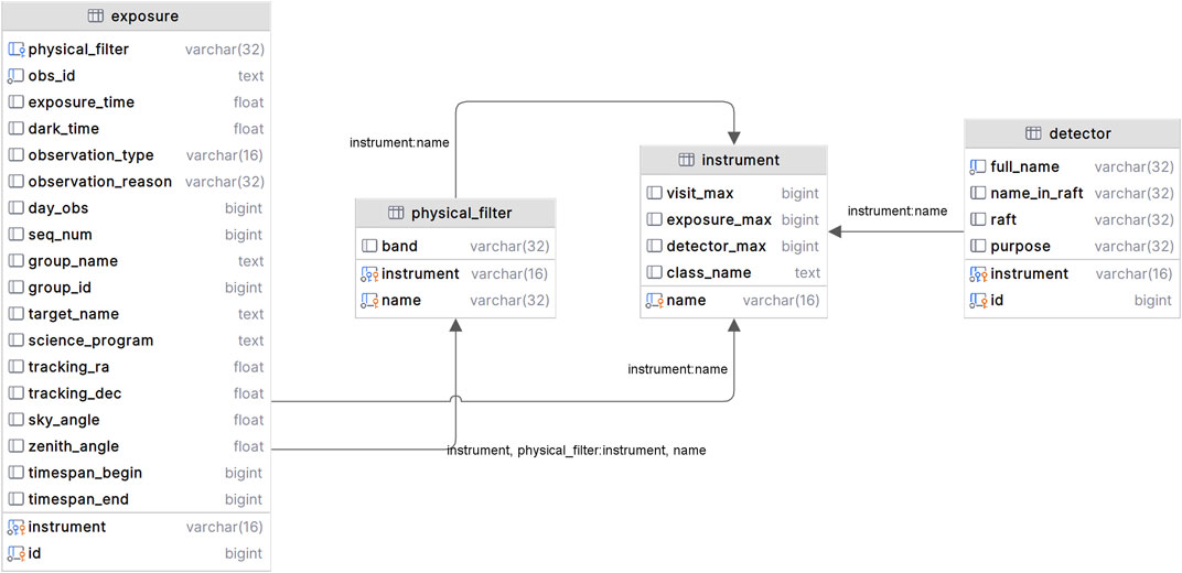
Figure 1. The LSST Science Pipelines utilizes SQLite3 to manage data. This figure illustrates the relationships between four tables: exposure, instrument, detector, and physical_filter. The relationships between these tables have been defined through the relations of primary and foreign keys. The keys marked with a yellow key pattern represent primary keys, while those with a blue key pattern represent foreign keys.

3.1.2 Interacting with data

Along with processing header information, efforts are also focused on enabling the LSST Science Pipelines to effectively process the actual data part of the raw data. This is achieved by integrating detailed camera and CCD information, along with other necessary information into the obs_mccd module. This integration covers aspects such as the layout of the focal plane, camera geometry, CCD dimensions, pixel size, and more. A practical reference for this is the camera.py⁶ script used for the HSC, which outlines the focal plane details and some CCD information.

In addition to camera.py, it is necessary for the LSST Science Pipelines to document specific details for each CCD amplifier, including the prescan region, science region, gain, saturation, readout direction, etc. Moreover, data about the telescope’s passband information—like filter names, coverage ranges, effective wavelengths, etc., — is crucial. The system also allows for the logging of comprehensive optical system transmission data, including filter transmission, CCD quantum efficiency, and atmospheric transmission.

In our obs_mccd, we use the information of the engineering diagram as reference to our prototype obs_package (shown in Figure 2), which outlines the CCD layout and gaps. In our prototype obs_package, assigned CCD IDs are assigned according to the following specification: from left to right, the first three CCDs are numbered as 0, 1, 2; the next row is sequentially numbered as 3, 4, 5; and the final row is sequentially numbered as 6, 7, 8. The CCD and amplifier details have been meticulously encoded. As an example, within the camera.py file, we specify that the instrument is equipped with nine CCDs, each having dimensions of 9,216 × 9,232 and a pixel size of 10 μm in both axes, with a pixel scale approximating 0.33′′. However, the actual layout of the focal plane may deviate from this design, for instance, during the processing of the engineering test data, we found numerous parameters needing modification. This update includes details such as the position of reference points (refpos_x(y)) and the physical coordinates of these points (offset_x(y)). Moreover, it was observed that the pixel scale is more accurately around 0.332″, slightly larger than the designed 0.33″, a discrepancy accounted for in the parameter transformDict. These values may require continual modification as changes occur during the operation and debugging of the instrument.

Figure 2

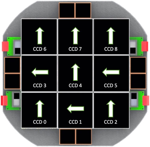
Figure 2. A sample CCD layout on the focal plane based on the engineering diagram of WFST (Lin et al., 2022). It specifies the CCD IDs, the gaps between any two adjacent CCDs, and the readout direction of each CCD.

3.2 Defining the pipeline for processing data

After establishing the interaction between raw data and the LSST Science Pipelines, the next critical step is defining a detailed pipeline. This process is more than just a linear progression; it involves the strategic assembly and coordination of various subtasks that cater to distinct requirements of data processing. The pipeline’s design is crucial because it dictates how data flows through the system, ensuring that each step is performed efficiently and accurately.

Pipelines are typically scripted in YAML files. An exemplary blueprint for a data release pipeline is the DRP-full.yaml⁷ which serves as a guideline. Within the scope of this paper, we specifically engage in singleFrame processing. This processing is an intricate procedure broken down into three pivotal subtasks: the correction of instrumental effects (ISR), the identification of key image features (characterizeImage), and the comprehensive calibration of the image (calibrate). Each of these subtasks plays a significant role in ensuring the integrity and quality of the processed data.

The singleFrame processing flow is systematically illustrated in Figure 3, where the visual representation aids in understanding the complex interactions and dependencies among different data processing stages. In this flowchart, rectangles are utilized to represent the inputs and outputs at various stages of the pipeline, symbolizing the transformation of raw data into refined, useable information. The orange ellipses highlight the operations applied to the data, indicating the dynamic nature of the processing steps.

Figure 3

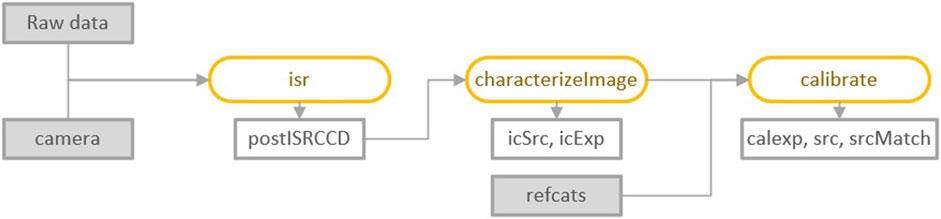
Figure 3. The flowchart of singleFrame processing, the rectangles represent input and output data, and the orange ellipses represent the operations to the data, the icSrc (SourceCatalog get by characterizeImage), icExp (ExposureF get by characterizeImage), calexp (calibrated exposureF) src (SourceCatalog get by calibrate) are all data types stored in the SQLite3 database.

This approach underscores the modular and flexible nature of pipeline design in the LSST Science Pipelines. Each subtask is carefully crafted to perform specific functions, and their collective execution leads to a comprehensive processing of the raw data. The design of these pipelines, therefore, is not just a technical task but also a conceptual challenge, requiring a deep understanding of both the astronomical phenomena being observed and the intricacies of data processing technologies.

The SQLite3 database plays a crucial role in managing the myriad of data products, such as postISRCCD, calexp, src and others, which are integral to the processing workflow. The presence of these data types within the dataset_type table of the SQLite3 database exemplifies the structured and methodical approach required for handling vast datasets typical in contemporary astronomical surveys. This database-driven approach ensures not only the integrity and accessibility of the data but also facilitates the complex computations and transformations that are fundamental to the LSST Science Pipelines.

3.3 Configuration information

Following the successful interaction of data with the LSST Science Pipelines and the construction of the data processing pipelines, the focus shifts to a critical aspect of pipeline execution: the customization and adjustment of task-specific configuration settings. This step is not merely a procedural requirement; it is a crucial aspect that ensures the pipeline’s performance is optimally tuned to the unique demands of the data and the specific objectives of the project.

Configuration settings act as the guiding parameters that dictate how each task within the pipeline processes the data. These settings can range from defining thresholds for data quality, setting parameters for image processing algorithms, to specifying criteria for data selection and analysis. Adjusting these configurations is a nuanced process that requires a deep understanding of both the nature of the data and the scientific goals of the project. It is where the theoretical aspects of astronomy, computational methods, and practical considerations of data handling converge.

Moreover, the configuration process is iterative and often involves a series of trials and refinements. This iterative approach allows for the fine-tuning of the pipeline to accommodate the inherent variability and complexity of astronomical data. It is a process that may involve consultation with domain experts, experimentation with different parameter settings, and extensive testing to evaluate the impacts of these configurations on the data processing outcomes.

In Section 4 that follows, some exposition on configuring and optimizing these pipelines is provided. The importance of this step in the data processing workflow cannot be overstated. Proper configuration is essential to achieving high-quality data processing outcomes, which in turn, has a direct impact on the reliability and validity of the scientific results.

4 Data processing with the pipelines

Following the development and implementation of the obs_mccd package, the initial phase in the data processing workflow entails the ingestion of data into the LSST Science Pipelines. For this purpose, we utilize version v23.0.1 of the LSST Science Pipelines, which has transitioned to using Generation 3 for data organization and task execution, moving away from the previous Generation 2 framework as introduced in Bosch et al. (2018). This shift marks a significant evolution in the way data is handled and processed.

The preparation process before the actual data processing involves a series of actions and checks to ensure smooth data interaction and processing. This preparatory phase includes tasks such as verifying data compatibility with the pipelines, ensuring all necessary metadata is correctly formatted and available, and setting up the initial parameters and configurations that the pipelines will use to process the data.

This stage is essential for laying a solid foundation for subsequent data processing steps. It ensures that the data is properly aligned with the requirements of the pipelines and that the pipelines are appropriately calibrated to handle the specific characteristics of the data. This preparation, as detailed below,

1. Create a Butler repository by the cmd butler create.

2. Register the mosaic CCD camera (MCCDCamera) into the Butler repository.

3. Ingest both the raw data and the calibration data by the cmd butler ingest-raws.

4. Group the exposures into visits by the cmd define-visits.

5. Ingest the reference catalogs.

Subsequently, we advanced to the data processing stage of our investigation. In this phase, we meticulously processed a dataset derived from a dense star field. These images were captured during the engineering test period of WFST. It is important to emphasize that this dataset was exclusively used to evaluate the feasibility of the pipeline and test our prototype obs_package, and does not ultimately reflect the quality of scientific images. This processing follows the singleFrame steps, as detailed in Figure 3. The upcoming sections provide a detailed account of the main data products generated from this processing, along with an evaluation by our QC system.

4.1 Instrumental signature removal (ISR)

Utilizing the calibration data that has been ingested, we create the master calibration files, specifically for bias and flat fields. This is executed through pipelines specifically engineered by the LSST Data Management team. The generation of the master bias is guided by the cpBias subtask⁸, while the creation of the master flat utilizes the cpFlat subtask⁹.

Subsequently, we establish the validity periods for these calibrations using the command certify-calibrations. This designation ensures that exposures captured during these periods will be processed using the appropriate bias and flat calibrations. Figure 4 displays the master flat that we have obtained, particularly employing twilight flats. The pipeline is adept at managing star trails, efficiently synthesizing multiple images to mitigate their effects.

Figure 4

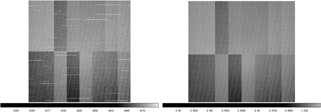
Figure 4. A sample flat image of CCD (ID 4), the left panel shows a single twilight flat, and the right panel is the resultant master flat combined by nine flats. The left image distinctly shows star trails, highlighting the initial quality of the single flat. The master flat demonstrates the effectiveness of the pipelines in mitigating such star trails. This improvement is achieved through the coaddition of multiple images, showcasing the capability of the pipelines to enhance image quality.

Beyond bias and flat, ISR includes adjustments for overscan areas, non-linearity in the detector response, crosstalk effects between different detector elements, and dark field corrections. Moreover, both variance and mask planes are generated for the subsequent data processing.

A key aspect of ISR is the identification and handling of defective pixels. Saturated and bad pixels are systematically detected, flagged, and then subjected to interpolation to minimize their impact on the final data. However, it is important to note that objects centered on these interpolated pixels might possess measurements that are deemed unreliable. To ensure data integrity, these objects are flagged in the catalogs to indicate potential measurement inaccuracies.

To preserve the integrity of the data and for future reference, a copy of the ISR-corrected images, along with the corresponding mask planes, is stored in the data repository. This archival ensures that the corrected data can be accessed and reanalyzed if necessary.

4.2 Image characterization (characterizeImage)

Once the instrumental signature has been removed from the raw image, the next step is to characterize the image, a process that involves a detailed assessment of its features. This step is visually represented in Figure 5 and entails a series of lower-level subtasks that are semi-iterative in nature. This means that many of these tasks are interdependent and cyclical. For instance, the source detection step can enhance background reduction, and conversely, more effective background reduction can lead to improved source detection.

Figure 5

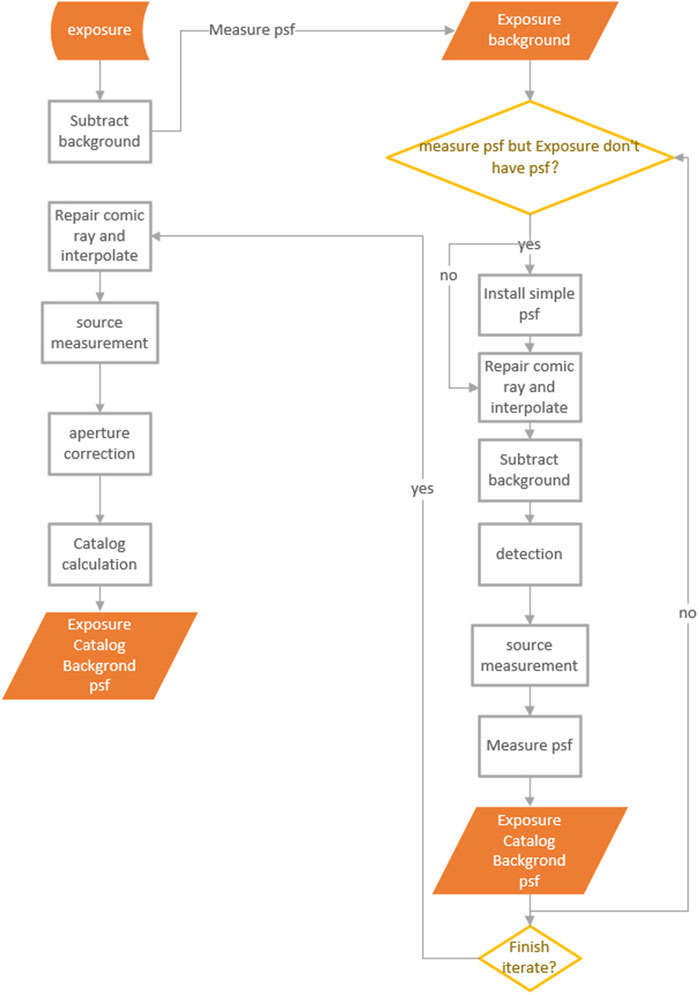
Figure 5. Flowchart of CharacterizeImageTask.

The workflow for this task is intricate and involves several stages. Initially, the image undergoes a thorough background estimation and subtraction, which is critical for accurately identifying and measuring the sources in the image. Following this, source detection algorithms are applied to identify potential objects within the image. After sources are detected, the next step typically involves measuring their properties, such as their positions, shapes, and fluxes.

The characterization process also includes the identification and masking of artifacts and anomalies in the image, such as cosmic rays or satellite trails, which can otherwise affect the accuracy of source detection and measurement. Additionally, the task involves refining the Point Spread Function (PSF) model, which describes how a point source (like a distant star) appears in the image. An accurate PSF model is crucial for precise photometric and astrometric measurements.

The semi-iterative nature of these tasks allows for continuous refinement and improvement of the image characterization. As the process iterates, the accuracy of source detection, background estimation, and other measurements gradually improves, leading to a more precise and detailed characterization of the image. This iterative process is key to extracting the maximum amount of useful information from raw images, paving the way for in-depth analysis and research. The task workflow is shown as follows:

1. Background Subtraction: The process begins with the initial reading of the original background, considering that background subtraction is iterative. After masking the image, the background is recalculated and refitted for different bins.

2. PSF-Related Information: The task evaluates if the image contains PSF-related information. In the absence of such data, and if the configuration does not require PSF measurement, a default two-dimensional Gaussian PSF (11 × 11 pixels, with a standard deviation of 1.5 pixels) is assigned to the image at that point.

3. Cosmic Ray Repair: This involves detecting cosmic rays by analyzing the brightness gradient. The identified cosmic rays are then masked and interpolated, followed by a re-calculation of the background.

4. Source Detection: The goal here is to identify a group of bright stars for constructing the PSF model, setting the detection threshold at 50σ. This step includes a nested task for updating the sky background after source detection, improving the fitting of the sky background.

5. Star/galaxy Classification This phase concentrates on determining if a source in the image is a point source or an extended one. This classification is based on extendedness, which is the difference between the PSF magnitude and the CModel magnitude of the source. Once classified, the source is then appropriately flagged in the system.

6. PSF Measurement: Measuring the PSF is iterative, with the number of iterations being selectable. Initially, if PSF information is absent, a simple Gaussian PSF is set. Subsequent tasks, like cosmic ray repair and source detection, are rerun, with the PSF being measured based on sources having a signal-to-noise ratio higher than 50σ.

7. Source Characteristic Measurement: In this step, various built-in algorithms can be chosen for calculating source features. For example, for flux calculation, options include aperture flux (base_CircularApertureFlux_12_0), PSF flux (base_PsfFlux), Gaussian flux (base_GaussianFlux), and CModel for galaxy photometry (Abazajian et al., 2004). Different algorithms can also be selected for measuring galaxy morphology.

8. Aperture Correction: This step is focused on aperture photometry, a fundamental technique in astrophysics for measuring the flux of astronomical objects. The process involves computing the ratios of different flux algorithm measurements to the measurement used for photometric calibration and using Chebyshev polynomials to interpolate.

Each of these steps is integral to the comprehensive processing and analysis of raw data, ensuring accurate and detailed characterization of the captured images.

4.2.1 Configurations of characterizeImage

Once the pipelines for data processing are outlined, the next step involves fine-tuning the configurations for various tasks, such as characterizeImage. This includes setting parameters for different stages of the process. For instance, during background subtraction, we can adjust the bin size for calculating the sky background, select the statistical method (like the default mean with clipping, or alternatives like mean without clipping or median), and choose the fitting algorithm for the sky background. Various functions can be used for this fitting, such as a single constant, a linear function, or spline functions like NATURAL_SPLINE or AKIMA_SPLINE, with AKIMA_SPLINE being the usual default. In tasks like PSF measurement and source characteristic measurement, we can also configure the size of the PSF. Similarly, for cosmic ray repair, settings include configuring the gradient to identify signals as cosmic rays and adjusting the threshold for source detection is also feasible.

In obs_mccd, it is essential to customize the configurations of different subtasks according to the specific characteristics of the instrument and the results obtained from preliminary data processing. This tailored approach ensures that the data processing is optimally aligned with the unique attributes of the instrument and the data, leading to more accurate and efficient processing outcomes.

4.2.2 PSF modeling and assessment

One of the most important products of characterizeImage is PSF. In the LSST Science Pipelines, PSF stars are selected via a k-means clustering algorithm (Bosch et al., 2018). PSF candidates are identified by rejecting objects with unusual brightness and size. After three iterations, PSF stars are determined across each CCD. In the output source catalogs, they are flagged as calib_psf_used=1. Intrinsically, the LSST Science Pipelines use PSFEx (Bertin, 2013) to model PSF stars on 41 × 41 − pixel postage stamps extracted from the post-ISR images. The PSF models on each CCD are established independently. In Figure 6, we show illustrative examples of PSF model residuals.

Figure 6

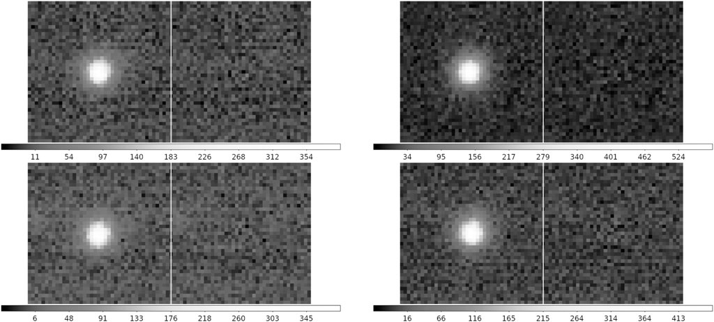
Figure 6. Four illustrative cases of PSF model residuals. The left part of each panel shows the original source image, while the right part displays the residuals remaining subsequent to the PSF subtraction. In the majority of instances, the residuals remaining after subtraction of the PSF model are negligible and merge with the background.

As a quality control, we fit a 2D Moffat function on each PSF star selected by the pipeline, and measure the FWHM to assess the PSF size. Meanwhile, we calculate the ellipticity of each PSF star from the characterizeImage output source catalogs. As a clarification, the ellipticity in this paper is defined using the distortion parameterization similar to (Bosch et al., 2018). In Figure 7, we demonstrate 2D plots of PSF FWHM and ellipticity for an example commissioning visit. The size and ellipticity are continuous across the entire focal plane. The central CCD has a relatively lower PSF size and ellipticity, whilst the PSF stars near the limbic and corner regions show larger values. In Figure 8, we plot the statistics of the FWHM and ellipticity.

Figure 7

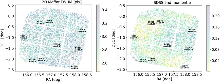
Figure 7. Example full FoV plots of PSF size (FWHM) and ellipticity. Each data point corresponds to the position of a PSF star. The color of the point represents the PSF size and ellipticity respectively. The median values of PSF size and ellipticity within each CCD are also labeled on the plots. Note: the plots are shown for validation of the QC system only.

Figure 8

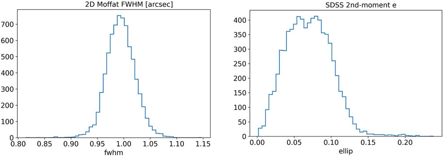
Figure 8. Example histogram plots of PSF size (FWHM) and ellipticity distribution. The FWHM is measured from the fitted 2D Moffat function on each PSF star selected by the pipeline. The ellipticity is calculated from the “SDSS 2nd-moments,” which are the photometric measurements using the SDSS algorithm as described in Lupton et al. (2001). This algorithm is integrated into the LSST Science Pipelines along with other photometric measurements and shape measurements. Note: the plots are shown for validation of the QC system only.

For the purpose of static cosmology, a desired median PSF in r-band should have a size smaller than 1.2 arcsec, and ellipticity lower than 0.13 according to the criteria described in Fu et al. (2022). In this example of commissioning r-band PSF assessment, most PSF stars have FWHM lower than 1.05 arcsec and ellipticity lower than 0.13. For the official survey data release in the future, adaptive optics and scheduling observations for optimal conditions can mitigate impacts from atmospheric conditions. Fine-tuning instrumental calibration, PSF modeling, artifact handling, and background modeling can also improve the data quality and reliability of photometric measurements. We wish to clarify that the example data presented in this paper serves solely for the purpose of validating and demonstrating the pipeline; it should not be interpreted as formal scientific results or as a reflection of the ultimate image quality.

4.3 Calibrate

Following the image characterization, the next step is to engage in the calibration process, akin to the procedures in characterizeImage. The calibrate stage involves several subtasks, initiating with source detection. Contrasting with the source detection in characterizeImage, which targets sources with a signal-to-noise ratio above 50σ, this phase broadens its scope to include all sources with a signal-to-noise ratio greater than 5σ. The subsequent stages of the calibration process encompass tasks such as source deblending, aperture correction, and the measurement of source characteristics. The procedure culminates with astrometry and photometry calibration. In our study, particular attention is given to assessing the efficacy of astrometric calibration within the data processing workflow.

4.3.1 SIP convention

Astrometry plays a fundamental role in image processing, and its quality significantly influences subsequent steps in data processing. One primary task of astrometry involves correcting geometric distortion caused by the optical system. The general process for handling distortion is described in (Calabretta et al., 2004), distortions can be corrected in either the initial pixel coordinate system or the intermediate pixel coordinate system. Subsequently, the corrected coordinate system obtained can be transformed into a spherical coordinate system and then into the desired celestial coordinate system. Distortion correction commonly involves polynomial fitting, with various polynomial specifications for this purpose. Examples include the polynomial specification output by SCAMP (Bertin, 2006) which is represented by PVi_j, and the SIP (Simple Imaging Polynomial) convention (Shupe et al., 2005). However, these two conventions are essentially interchangeable (Shupe et al., 2012), the LSST Science Pipelines we employ adopt the SIP convention, which is denoted by Eqs 1–3:

$\left(\begin{array}{c}\hfill x\hfill \\ \hfill y\hfill \end{array}\right)=\left(\begin{array}{cc}\hfill CD1\text{\_}1\hfill & \hfill CD1\text{\_}2\hfill \\ \hfill CD2\text{\_}1\hfill & \hfill CD2\text{\_}2\hfill \end{array}\right)\left(\begin{array}{c}\hfill u+f\left(u,v\right)\hfill \\ \hfill v+g\left(u,v\right)\hfill \end{array}\right)(1)$

$f\left(u,v\right)={\displaystyle \sum _{p,q}}A\text{\_}p\text{\_}q{u}^p{v}^q,p+q<=order(2)$

$g\left(u,v\right)={\displaystyle \sum _{p,q}}B\text{\_}p\text{\_}q{u}^p{v}^q,p+q<=order(3)$

4.3.2 Source matching

Fitting the SIP polynomial, which describes distortion, necessitates accurately determining the actual positions of stars in an image. This step requires correlating the stars detected in the image with their counterparts in the reference catalogs. The typical method for achieving this is by creating and comparing patterns constructed from stars in both the image and the reference catalog. This comparison process is known as “matching.”

One common approach to matching is the construction of triangles using stars and then comparing specific geometric properties of these triangles. For example, a method involves comparing the ratio of the longest to the shortest side of the triangles, along with the cosine value of the included angles, as described by Groth (1986). Other methods have evolved from this, varying in the attributes compared. For instance, Valdes et al. (1995) developed a technique involving the comparison of ratios like b/a and c/a in patterns from two star catalogs, where a, b, and c represent the sides of the triangle in decreasing lengths.

These matching techniques are crucial for astrometric calibration, ensuring that the observed positions of stars align with their known positions in the celestial sphere, thereby enabling accurate distortion modeling in astronomical imaging. In addition to triangles, various other geometric patterns are employed for the matching process. For instance, the Optimistic Pattern Matching B (OPMb) algorithm uses a pinwheel pattern, as depicted in Figure 3 of the study by Tabur (2007). The matching process in OPMb involves comparing the separations of stars and their position angles (PA) relative to a central star in the pattern.

However, OPMb encounters difficulties in regions with high stellar density. To address this, the LSST Science Pipelines have adapted a modified version of this algorithm, known as the Pessimistic Pattern Matcher B (PPMb). PPMb is designed to be more robust in dense star fields. The steps of implementing the PPMb algorithm can be summarized as follows:

1. Determine the center of the loaded reference catalog based on the telescope pointing and rotation angle. The size of the catalog is determined by the geometric description of the instrument in camera.py. During the loading process, a sky region marginally larger than described in camera.py is loaded, followed by the application of proper motion correction to the loaded reference star catalog.

2. In the source detection step, star catalogs are sorted by brightness in descending order for both the image and reference catalogs. The position of each star is then converted into x, y, z coordinates within a unit sphere coordinate system. Based on brightness, pinwheel patterns are created separately for the image and reference catalogs, facilitating the alignment and comparison process in astrometric analysis.

3. Automatically compute the matching tolerance dist_tol. Employ the previously constructed patterns and utilize cKDTree to find the two most similar patterns in the image catalog and calculate the average difference between these two patterns. Repeat the same process for the reference catalog. The final tolerance value is determined by selecting the smaller of the two differences. During the matching process of the patterns in the image catalogs and the reference catalog, the difference in spokes’ lengths between two patterns must be smaller than the tolerance value to consider them as the same group of stars.

4. Set additional tolerances for the subsequent matches, including shift and rotation. During the iterative process, automatically relax the criteria when there are no matches.

5. The matching process starts with the catalog from the image, selecting reference stars for comparison based on their brightness. A spoke pattern is created using star pairs from the image, and similar patterns from the reference catalog are identified within a certain tolerance range as calculated in the second step. After this initial filtering, a further, more detailed comparison will be conducted, ultimately resulting in a list of matches, which is used for fitting the SIP polynomial for astrometric calibration.

We processed 50 exposures from a dense star field. Gaia DR3 catalog (Brown et al., 2021) was used as the reference catalog to test the correction quality of geometric distortion. Figures 9, 10 showcases the comparison between corrections using fifth-order and third-order SIP polynomials for distortion fitting. We divided each CCD into 16 × 16 bins, with the red line segment indicating a 0.1-pixel residual. For the central CCD (ID 4), employing a third-order polynomial to correct geometric distortions yields relatively satisfactory results. The outcomes derived from fitting the geometric distortions of the central CCD with a fourth-order polynomial are approximately equivalent to those obtained with a third-order polynomial, and employing a fifth-order polynomial, nonetheless, can improve the precision of the fit. However, for CCDs further from the center, the third-order polynomial fitting showed significant residuals, suggesting inadequate correction of distortion. In contrast, the fifth-order polynomial fitting more effectively accounted for the distortion. Based on these observations, we opted for a fifth-order polynomial for SIP fitting in our data processing. Figure 11 also present the distribution of mean on-sky distance and scatter for all these CCDs. After processing with the LSST science pipelines, the HSC’s systematic error is approximately 10 mas. Our processed final results are on the same order of magnitude as those of the HSC.

Figure 9

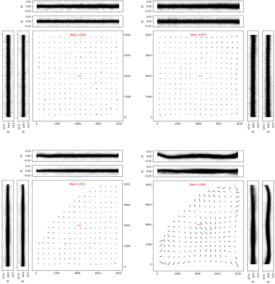
Figure 9. From top to bottom, the geometric distortion maps for CCD ID 4 and 0. The left panel displays residuals using the fifth-order SIP polynomial while the right panel shows results using the third-order SIP polynomial. The size of the residual vectors is magnified by a factor of 4,000, and the red vector in the center represents a residual of 0.1 pixel. The median of these vectors is displayed above the image. We also show the residual trends along the X and Y-axes. Units are in pixels.

Figure 10

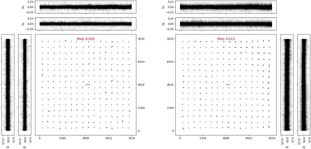
Figure 10. The geometric distortion maps for CCD ID 4 processed by two different pipelines. The left panel displays residuals using the LSST science pipelines while the right panel shows results using our in-house pipelines. The size of the residual vectors is magnified by a factor of 4,000, and the red vector in the center represents a residual of 0.1 pixel. The median of these vectors is displayed above the image. We also show the residual trends along the X and Y-axes. Units are in pixels.

Figure 11

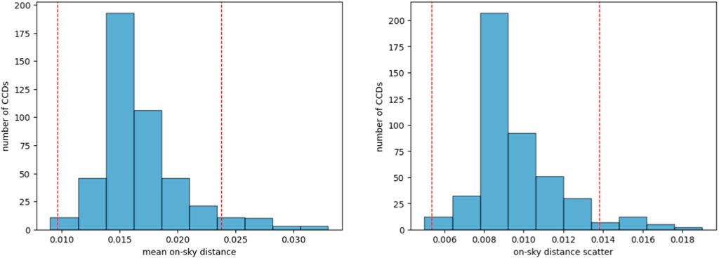
Figure 11. The distribution of mean on-sky distance and scatter is presented, with the red line indicating the 2σ level of this distribution. The units on the horizontal axis are in arcseconds.

In addition to employing the LSST pipelines for astrometry, we also utilize our in-house developed pipeline, which is based on Sextractor (Bertin and Arnouts, 1996), PSFEx, and SCAMP, to perform tasks such as source detection, PSF construction, and astrometry. Similar configurations are applied to process the results of the same data batch. For instance, we match stars with a signal-to-noise ratio greater than 40 and similarly employ a fifth-order polynomial for fitting. The final outcomes for the correction of geometric distortions are akin between the two approaches, the median average of nine CCDs obtained from processing with the LSST pipeline is 0.011″, while the median average yielded by our in-house pipeline stands at 0.016′′. Both outcomes are satisfactory and exhibit a small discrepancy. However, considering that the LSST pipeline not only executes the aforementioned tasks but also offers a plethora of additional features and facilitates convenient data management through databases, we plan to adopt the LSST pipeline for data processing in future endeavors.

As previously stated, the sample data showcased in this paper is utilized strictly for the purposes of validating the pipeline and testing the astrometric calibration algorithms and configurations. It is important to note that these examples are not indicative of finalized scientific outcomes or the definitive quality of images.

5 Summary

In this study, with guidance and resources provided by the LSST community, including valuable comments and tutorials, and inspired by the successful implementation of these pipelines by the HSC team, we have adopted the LSST Science Pipelines for processing data from a mosaic CCD instrument. To showcase the workflow, we demonstrate the CCD-level processing of raw images from the engineering test of WFST. This paper outlines our development of the obs_mccd package and the execution of various data processing operations enabled by this package, such as ISR, characterizeImage, and calibrate. Additionally, we assess the outcomes of our data processing workflow, focusing on the PSF modeling and the correction of geometric distortion. Our findings recommend using a fifth-order polynomial for effective distortion correction in a realistic dataset.

The LSST Science Pipelines have proven their advanced capabilities and high-quality data processing, as evidenced by the HSC. In our data validation, data processing was conducted on a computer equipped with an AMD EPYC 7763 64-core processor and 1008 GB RAM. We present the wall-clock time for processing 450 CCDs at each stage on a single core: the calibration step averaged 293.0 s, the characterizeImage required an average of 123.2 s, and ISR took 77.3 s. On average, processing a single image took approximately 8 min. The obs_package makes the execution of LSST pipeline tasks more accessible to our instrument. Our work aims to serve as a practical guide and introduction for others interested in leveraging the LSST Science Pipelines for their observational data.

Furthermore, we recognize the untapped potential of the LSST Science Pipelines. They offer a wealth of features, such as utilizing multi-epoch data for improved calibrations and exploring functionalities like coaddition and forced photometry. Our future work will delve into these additional capabilities, expanding the scope and impact of our research with the LSST Science Pipelines.

Data availability statement

The data analyzed in this study is subject to the following licenses/restrictions: The data used for pipeline validation is from the engineering test of WFST and is not public due to relevant data policy. The data may be available upon request. Requests to access these datasets should be directed to BL, byliu@pmo.ac.cn.

Author contributions

YH: Writing–original draft, Writing–review and editing. CY: Writing–original draft, Writing–review and editing. MZ: Writing–original draft, Writing–review and editing. YC: Writing–original draft, Writing–review and editing. BL: Writing–original draft, Writing–review and editing.

Funding

The author(s) declare that financial support was received for the research, authorship, and/or publication of this article. This study is supported by the National Key Research and Development Program of China (2023YFA1608100), and the Cyrus Chun Ying Tang Foundations. YH acknowledges the scholarship from the Cyrus Chun Ying Tang Foundations.

Acknowledgments

We thank the referees and Prof. Xianzhong Zheng and Prof. Min Fang at Purple Mountain Observatory for their supervision and constructive discussion. We extend our heartfelt gratitude to the LSST community and the Data Management team. Their invaluable contributions, ranging from the development of cutting-edge tools to the supportive environment they foster, have been instrumental in our research. We would like to express our gratitude to the LSST Community Forum and its members for their enthusiastic, proactive, and prompt responses in addressing our questions and helping us navigate challenges encountered during the utilization and modification of LSST science pipelines. This paper makes use of LSST Science Pipelines software developed by the Vera C. Rubin Observatory. We thank the Rubin Observatory for making their code available as free software at https://pipelines.lsst.io.

Conflict of interest

The authors declare that the research was conducted in the absence of any commercial or financial relationships that could be construed as a potential conflict of interest.

The reviewer JY shared authors YH, CY, YC second affiliation at the time of review.

Publisher’s note

All claims expressed in this article are solely those of the authors and do not necessarily represent those of their affiliated organizations, or those of the publisher, the editors and the reviewers. Any product that may be evaluated in this article, or claim that may be made by its manufacturer, is not guaranteed or endorsed by the publisher.

Footnotes

¹https://pipelines.lsst.io/

²https://github.com/lsst/obs_subaru

³https://pipelines.lsst.io/modules/lsst.obs.base/creating-an-obs-package.html

⁴https://github.com/lsst/astro_metadata_translator/blob/main/python/ astro_metadata_translator/properties.py

⁵https://github.com/lsst/astro_metadata_translator/blob/main/python/ astro_metadata_translator/translators/fits

⁶https://github.com/lsst/obs_subaru/blob/main/hsc/camera/camera.py

⁷https://github.com/lsst/drp_pipe/blob/main/pipelines/_ingredients/ DRP-full.yaml

⁸https://github.com/lsst/cp_pipe/blob/23.0.1/pipelines/cpBias.yaml

⁹https://github.com/lsst/cp_pipe/blob/23.0.1/pipelines/cpFlat.yaml

References

Abazajian, K., Adelman-McCarthy, J. K., Agüeros, M. A., Allam, S. S., Anderson, K., Anderson, S. F., et al. (2004). The second data release of the sloan digital sky survey. AJ 128, 502–512. doi:10.1086/421365

CrossRef Full Text | Google Scholar

Abbott, B. P., Abbott, R., Abbott, T., Abernathy, M., Acernese, F., Ackley, K., et al. (2016). Observation of gravitational waves from a binary black hole merger. Phys. Rev. Lett. 116, 061102. doi:10.1103/physrevlett.116.061102

PubMed Abstract | CrossRef Full Text | Google Scholar

Aihara, H., AlSayyad, Y., Ando, M., Armstrong, R., Bosch, J., Egami, E., et al. (2019). Second data release of the hyper suprime-cam subaru strategic Program. PASJ 71, 114. doi:10.1093/pasj/psz103

CrossRef Full Text | Google Scholar

Aihara, H., Armstrong, R., Bickerton, S., Bosch, J., Coupon, J., Furusawa, H., et al. (2018). First data release of the hyper suprime-cam subaru strategic Program. PASJ 70, S8. doi:10.1093/pasj/psx081

CrossRef Full Text | Google Scholar

Bertin, E. (2006). “Automatic astrometric and photometric calibration with SCAMP,” in Astronomical data analysis software and systems XV. Editors C. Gabriel, C. Arviset, D. Ponz, and S. Enrique (San Francisco: Astronomical Society of the Pacific Conference Series), 351, 112.

Google Scholar

Bertin, E. (2013). Psfex: point spread function extractor. Astrophys. Source Code Libr. 1301, 001.

Google Scholar

Bertin, E., and Arnouts, S. (1996). SExtractor: software for source extraction. Astron. Astrophys. Suppl. Ser. 117, 393–404. doi:10.1051/aas:1996164

CrossRef Full Text | Google Scholar

Blum, R. D., Burleigh, K., Dey, A., Schlegel, D. J., Meisner, A. M., Levi, M., et al. (2016). “The DECam legacy survey,” in American astronomical society meeting abstracts #228 (American Astronomical Society Meeting Abstracts).

Google Scholar

Bosch, J., AlSayyad, Y., Armstrong, R., Bellm, E., Chiang, H.-F., Eggl, S., et al. (2019). “An overview of the LSST image processing pipelines,” in Astronomical data analysis software and systems XXVII. Editors P. J. Teuben, M. W. Pound, B. A. Thomas, and E. M. Warner (San Francisco: Astronomical Society of the Pacific Conference Series), 523, 521. doi:10.48550/arXiv.1812.03248

CrossRef Full Text | Google Scholar

Bosch, J., Armstrong, R., Bickerton, S., Furusawa, H., Ikeda, H., Koike, M., et al. (2018). The Hyper Suprime-Cam software pipeline. PASJ 70, S5. doi:10.1093/pasj/psx080

CrossRef Full Text | Google Scholar

Brown, A. G., Vallenari, A., Prusti, T., De Bruijne, J., Babusiaux, C., Biermann, M., et al. (2021). Gaia early data release 3. Astronomy Astrophysics 649, A1. doi:10.1051/0004-6361/202141135

CrossRef Full Text | Google Scholar

Calabretta, M. R., Valdes, F., Greisen, E. W., and Allen, S. L. (2004). “Representations of distortions in FITS world coordinate systems,” in Astronomical data analysis software and systems (ADASS) XIII. Editors F. Ochsenbein, M. G. Allen, and D. Egret (San Francisco: Astronomical Society of the Pacific Conference Series), 314, 551.

Google Scholar

Chang, C., Wang, M., Dodelson, S., Eifler, T., Heymans, C., Jarvis, M., et al. (2018). A unified analysis of four cosmic shear surveys. Mon. Notices R. Astronomical Soc. 482, 3696–3717. doi:10.1093/mnras/sty2902

CrossRef Full Text | Google Scholar

Dalal, R., Li, X., Nicola, A., Zuntz, J., Strauss, M. A., Sugiyama, S., et al. (2023). Hyper suprime-cam year 3 results: cosmology from cosmic shear power spectra. Phys. Rev. D. 108, 123519. doi:10.1103/PhysRevD.108.123519

CrossRef Full Text | Google Scholar

Erben, T., Hildebrandt, H., Miller, L., van Waerbeke, L., Heymans, C., Hoekstra, H., et al. (2013). Cfhtlens: the Canada–france–Hawaii telescope lensing survey – imaging data and catalogue products. Mon. Notices R. Astronomical Soc. 433, 2545–2563. doi:10.1093/mnras/stt928

CrossRef Full Text | Google Scholar

Fu, S., Dell’Antonio, I., Chary, R.-R., Clowe, D., Cooper, M. C., Donahue, M., et al. (2022). Lovoccs. i. survey introduction, data processing pipeline, and early science results. Astrophysical J. 933, 84. doi:10.3847/1538-4357/ac68e8

CrossRef Full Text | Google Scholar

Fu, S., Dell’Antonio, I., Escalante, Z., Nelson, J., Englert, A., Helhoski, S., et al. (2024). Lovoccs – ii. weak lensing mass distributions, red-sequence galaxy distributions, and their alignment with the brightest cluster galaxy in 58 nearby x-ray-luminous galaxy clusters. arXiv.

Google Scholar

Groth, E. J. (1986). A pattern-matching algorithm for two-dimensional coordinate lists. AJ 91, 1244–1248. doi:10.1086/114099

CrossRef Full Text | Google Scholar

Gunn, J. E., Siegmund, W. A., Mannery, E. J., Owen, R. E., Hull, C. L., Leger, R. F., et al. (2006). The 2.5 m telescope of the sloan digital sky survey. AJ 131, 2332–2359. doi:10.1086/500975

CrossRef Full Text | Google Scholar

Ivezić, Ž., Kahn, S. M., Tyson, J. A., Abel, B., Acosta, E., Allsman, R., et al. (2019). LSST: from science drivers to reference design and anticipated data products. ApJ 873, 111. doi:10.3847/1538-4357/ab042c

CrossRef Full Text | Google Scholar

Jenness, T., Bosch, J. F., Salnikov, A., Lust, N. B., Pease, N. M., Gower, M., et al. (2023). “The Vera C. Rubin Observatory Data Butler and pipeline execution system,” in Proc. SPIE 12189, Software and Cyberinfrastructure for Astronomy VII. August 29, 2022, 1218911. doi:10.1117/12.2629569

CrossRef Full Text | Google Scholar

Jurić, M., Kantor, J., Lim, K. T., Lupton, R. H., Dubois-Felsmann, G., Jenness, T., et al. (2017). “The LSST data management system,” in Astronomical data analysis software and systems XXV. Editors N. P. F. Lorente, K. Shortridge, and R. Wayth (San Francisco: Astronomical Society of the Pacific Conference Series), 512, 279. doi:10.48550/arXiv.1512.07914

CrossRef Full Text | Google Scholar

Lin, Z., Jiang, N., and Kong, X. (2022). The prospects of finding tidal disruption events with 2.5-m Wide-Field Survey Telescope based on mock observations. Mon. Notices R. Astronomical Soc. 513, 2422–2436. doi:10.1093/mnras/stac946

CrossRef Full Text | Google Scholar

Lupton, R., Gunn, J. E., Ivezić, Z., Knapp, G. R., and Kent, S. (2001). “The SDSS imaging pipelines,” in Astronomical data analysis software and systems X. Editors J. Harnden, F. R., F. A. Primini, and H. E. Payne (San Francisco: Astronomical Society of the Pacific Conference Series), 238, 269. doi:10.48550/arXiv.astro-ph/0101420

CrossRef Full Text | Google Scholar

Magnier, E., Kaiser, N., and Chambers, K. (2006). “The pan-starrs ps1 image processing pipeline,” in The Advanced Maui Optical and Space Surveillance Technologies Conference, Wailea, Maui, Hawaii, September 10-14, 2006 (Maui: The Maui Economic Development Board), 50.

Google Scholar

Massey, P. (1997). A user’s guide to ccd reductions with iraf. Tucson: National Optical Astronomy Observatory.

Google Scholar

Miller, L., Kitching, T., Heymans, C., Heavens, A., and Van Waerbeke, L. (2007). Bayesian galaxy shape measurement for weak lensing surveys–i. methodology and a fast-fitting algorithm. Mon. Notices R. Astronomical Soc. 382, 315–324. doi:10.1111/j.1365-2966.2007.12363.x

CrossRef Full Text | Google Scholar

Mullaney, J. R., Makrygianni, L., Dhillon, V., Littlefair, S., Ackley, K., Dyer, M., et al. (2021). Processing GOTO data with the Rubin observatory LSST science pipelines I: production of coadded frames. PASA 38, e004. doi:10.1017/pasa.2020.45

CrossRef Full Text | Google Scholar

Schirmer, M. (2013). Theli: convenient reduction of optical, near-infrared, and mid-infrared imaging data. Astrophysical J. Suppl. Ser. 209, 21. doi:10.1088/0067-0049/209/2/21

CrossRef Full Text | Google Scholar

Shupe, D. L., Laher, R. R., Storrie-Lombardi, L., Surace, J., Grillmair, C., Levitan, D., et al. (2012). “More flexibility in representing geometric distortion in astronomical images,” in Software and cyberinfrastructure for astronomy II. Editors N. M. Radziwill, and G. Chiozzi (Bellingham: Society of Photo Optical Instrumentation Engineers), 8451, 84511M. doi:10.1117/12.925460

CrossRef Full Text | Google Scholar

Shupe, D. L., Moshir, M., Li, J., Makovoz, D., Narron, R., and Hook, R. N. (2005). “The SIP convention for representing distortion in FITS image headers,” in Astronomical data analysis software and systems XIV. Editors P. Shopbell, M. Britton, and R. Ebert (San Francisco: Astronomical Society of the Pacific Conference Series), 347, 491.

Google Scholar

Stetson, P. B. (1987). Daophot: a computer program for crowded-field stellar photometry. San Francisco: Publications of the Astronomical Society of the Pacific, 191.

CrossRef Full Text | Google Scholar

Tabur, V. (2007). Fast algorithms for matching CCD images to a stellar catalogue. PASA 24, 189–198. doi:10.1071/AS07028

CrossRef Full Text | Google Scholar

Valdes, F., and Gruendl, R. (2014). The decam community pipeline. Astronomical Data Analysis Softw. Syst. XXIII 485, 379.

Google Scholar

Valdes, F. G., Campusano, L. E., Velasquez, J. D., and Stetson, P. B. (1995). FOCAS automatic catalog matching algorithms. PASP 107, 1119. doi:10.1086/133667

CrossRef Full Text | Google Scholar

Wang, T., Liu, G., Cai, Z., Geng, J., Fang, M., He, H., et al. (2023). Science with the 2.5-meter wide field survey telescope (WFST). Sci. China Phys. Mech. Astronomy 66, 109512. doi:10.1007/s11433-023-2197-5

CrossRef Full Text | Google Scholar