Spatial profiles of magnetosheath parameters under different IMF orientations: THEMIS observations

Modification of the solar wind parameters at the bow shock (BS) and through the magnetosheath (MSH) is essential for the solar wind–magnetosphere interaction chain. The present study uses two approaches to determine the spatial profile of magnetic field strength and plasma parameters and their fluctuations along the Sun-Earth line under different interplanetary magnetic field (IMF) orientations with an emphasis on radial IMF conditions. The first method is based on the superposed epoch analysis of all the complete THEMIS MSH crossings between 2007 and 2010. The second approach uses the distance of the observing spacecraft from the model magnetopause (MP) expressed in units of an MSH thickness for all THEMIS observations. The results of both these analyses are consistent, and their comparison with simulations reveals the following features: 1) the sign of the IMF north-south component has a negligible effect on the spatial profile of the magnetic field strength or plasma parameters as well as on the level of fluctuations; 2) the ion temperature is enhanced for a radial MF and it is nearly isotropic throughout MSH; 3) the fluctuation level of plasma parameters just downstream BS is enhanced under a radial IMF, but it gradually decreases toward MP to a value typical for other IMF orientations; 4) magnetic field fluctuations are enhanced by a factor of 1.7 in the whole magnetosheath when IMF points radially.

1 Introduction

The Earth’s magnetosphere is embedded in the solar wind and adjusts itself to the prevailing solar wind conditions. Numerous previous studies have investigated the relations between the magnetospheric phenomena and solar wind observations recorded at the L1 point. However, the solar wind plasma and interplanetary magnetic field (IMF) undergo changes at the bow shock (BS) and pass through the magnetosheath (MSH) before reaching the magnetosphere. Thus, the changes of solar wind parameters in MSH on large and small scales directly affecting the magnetosphere should be studied deeply. Despite the importance of MSH processes, relatively few large-scale statistical studies have been devoted to the situation in the entire MSH. It might be due to the continuous motion of BS and magnetopause (MP) locations, causing difficulty in the determination of the exact location of these boundaries for a particular MSH observation.

Hydrodynamic models of MSH plasma and magnetic field profiles (Spreiter et al., 1966; Spreiter and Stahara, 1980) predict that the velocity decreases from BS toward MP, whereas the density and temperature increase. Magnetohydrodynamic simulations confirm these global MSH profiles (e.g., Liu et al., 2015). However, multipoint observation studies (e.g., Zastenker et al., 2002) show that the hydrodynamic model could only predict the large-scale MSH profile. Still, it cannot reproduce the small-scale structures where values of particular plasma parameters can differ from the predicted values by a factor of 5 (Němeček et al., 2000). Such structures can be generated in MSH, and their generation processes would depend on the IMF cone angle (arccos (|B_X|/|B|)) because the hydrodynamic model predictions are less accurate when the IMF vector is aligned with a solar wind flow (Němeček et al., 2000). The follow-up study of Němeček et al. (2002) further points out that the IMF orientation strongly influences the dayside MSH radial profile of the ion flux.

Several statistical studies (Paularena et al., 2001; Longmore et al., 2005) have applied the MSH interplanetary medium reference frame (Bieber and Stone, 1979) to solve the problem of boundary locations. Their global studies have shown a dawn-dusk asymmetry in the plasma density; it is larger at the dawn side, whereas the flow speed is higher on the dusk side, and this asymmetry depends on the solar cycle. Dimmock and Nykyri (2013) applied the same method to the THEMIS data and showed the asymmetries of the magnetic field, density, and flow speed in MSH. The results also reveal that the IMF orientation plays a role in forming the MSH magnetic field strength profile. Ma et al. (2020) used more than 12 years of THEMIS data to investigate MSH and magnetospheric asymmetries and compare them with BATS-R-US simulations. The results show that the plasma density is higher at the region close to MP during northward IMF (nIMF) than southward IMF (sIMF) orientation.

One of the most critical parameters for modifying upstream solar wind parameters at BS is an angle between the IMF vector and the normal to the BS surface (ϴ_BN) (Czaykowska et al., 2000). BS influences only the components perpendicular to the shock normal; therefore, the solar wind parameters would exhibit more significant changes downstream quasi-perpendicular shocks (ϴ_BN > 45°) than downstream quasi-parallel shocks (ϴ_BN < 45°). The proton temperature is nearly isotropic downstream of the quasi-parallel shock, but the increase of the temperature anisotropy is typical for the downstream of quasi-perpendicular shocks. Temperature anisotropy can directly affect plasma instability excitation and growth rates (Gary et al., 1993), forming more waves in the downstream region of perpendicular shocks. On the other hand, reflected particles move upstream along the magnetic field line under the quasi-parallel shock topology, generating a foreshock region in front of BS. The highly disturbed solar wind in the foreshock ultimately propagates into MSH. Different kinds of transients (e.g., Xirogiannopoulou et al., 2024) are generated in the foreshock and influence the downstream structures (see Zhang et al., 2022 for a review). For example, the hot flow anomalies originating due to the interaction of an IMF tangential discontinuity substantially decrease the dynamic pressure (P_d) and cause a local MP expansion (Šafránková et al., 2012). Similar effects can result from the interaction of MP with the MSH jets (Němeček et al., 2023).

In addition to the different types of bow shock and foreshock effects, the plasma and magnetic field profiles are also influenced by the local structures in MSH, such as the depletion layer (Midgley and Davis, 1963). The depletion layer in front of MP is characterized by a strong magnetic field and low plasma density. Such structures also depend on the IMF orientations; the depletion layer usually appears when the IMF points northward because an inward flow compresses the magnetic field, and the increased magnetic pressure pushes the plasma away along the magnetic field lines, but dayside reconnection destroys the depletion layer under sIMF (e.g., Anderson and Fuselier, 1993; Šafránkova et al., 2009). On the other hand, MP reconnection occurs at the lobe region, and it creates a dense low-latitude boundary layer on the magnetospheric side of the MP and/or MSH boundary layer on the opposite side under nIMF, but these layers are missing for sIMF (Němeček et al., 2015). Zhang et al. (2019) studied the plasma parameters in MSH and their influence on the reconnection rate. They conclude that the IMF clock angle, MSH plasma β, and the solar wind sound Mach number are significant factors controlling the MP reconnection rate.

Based on the above results, we know that the IMF orientation plays an important role in the determination of the MSH environment. Aside from the south-north magnetic orientation, the radial IMF (rIMF) component is also essential because IMF points nearly radially approximately 10%–15% of the total observation time (Pi et al., 2014). RIMF shifts the foreshock toward the BS nose, and the foreshock covers almost the whole dayside magnetosphere (Blanco-Cano et al., 2009). Foreshock transients, such as spontaneous hot flow anomalies, foreshock bubbles, etc., are more likely to be generated in this huge region and influence the magnetosphere. RIMF forms a thinner MSH because of the low Mach number (Pi et al., 2014; Wang et al., 2020), and the magnetic field at the subsolar MSH would be low due to the low compression ratio at the quasi-parallel BS (Czaykowska et al., 2000). The radial (B_X) component converts into B_Y and B_Z components in MSH (Pi et al., 2016), and it leads to different B_Z orientations in the north and south hemispheres and the simultaneous appearance of subsolar and lobe reconnection locations in different hemispheres (Pi et al., 2017). This asymmetric reconnection can generate a thick MSH boundary layer (Pi et al., 2018).

Several simulation results show that the pressure profiles, including total (P_tot), dynamic (P_d), thermal (P_t), and magnetic (P_b) pressures across MSH reflect different IMF orientations (e.g., Samsonov et al., 2012; Wang et al., 2018). The simulations reveal three interesting results: 1) P_t increases with a distance from BS for sIMF, but it shows a bump in MSH for nIMF because the depletion layer decreases P_t near MP; 2) the ratio between upstream and downstream P_tot across BS changes with upstream P_d; and P_tot decreases significantly after the BS crossing for a large P_d; 3) P_tot roughly remains constant across the whole MSH for nIMF, but it decreases during the MSH pass for sIMF (see Figs. 8, 9 in Wang et al. (2018)). Samsonov et al. (2012) compare the results of isotropic and anisotropic MHD models and show that the anisotropic temperature modeling leads to a lower effective P_tot under rIMF than the nIMF orientation. These phenomena have not yet been confirmed by observations.

In summary, we know many effects of changing the incoming solar wind parameters before reaching MP, and most depend on the IMF orientation. However, the effects themselves or whether they will occur in the whole MSH still need to be quantified, especially for rIMF. Therefore, we use 4 years of THEMIS observations to study the MSH spatial profiles of the plasma parameters, magnetic field strength, and pressure components and discuss the influence of IMF orientations on them. After the introduction, section 2 describes the data used in this study, section 3 contains the data processing methods, and section 4 is devoted to the results obtained by two different approaches. The discussion and conclusions are presented in sections 5 and 6.

2 Data used

We use measurements from all probes of the THEMIS mission (Sibeck and Angelopoulos, 2008) from 2007 to 2010 because these probes with apogees ranging from 10 to 30 R_E provide frequent MSH observations during the selected period. The electrostatic analyzer (ESA; McFadden et al., 2008) records the plasma data continuously with a 3-s resolution. In the target region of our study, ESA often switches between the solar wind and magnetospheric modes, which could influence the statistical results. Therefore, the onboard moments (MOM) calculated from data gathered in the magnetospheric mode are selected. The fluxgate magnetometer (FGM; Auster et al., 2008) records the magnetic field vector with even higher time resolution, but all measurements mentioned above are averaged into 1-min intervals.

3 Methodology

Each statistical MSH study faces the task of determining the distance between the MSH point of observation and MP/BS without continuously recording MP/BS locations. To solve this task, we apply two approaches and check the consistency of the results.

3.1 Superposed epoch analysis

In the first approach, we visually checked THEMIS B (THB) and THEMIS C (THC) data plots during 2007–2010 to select the complete subsolar MSH crossings for different IMF orientations. Such crossing is chosen using the following steps: 1) we identified all THB and THC trajectories when the angle between the spacecraft position vector and the Sun-Earth line is smaller than 30°; 2) the complete MSH crossing (complete in here means that both the MP and BS are observed) is fully covered by the data. If there are multiple BS and MP crossings, the first (or last, based on the direction of the satellite motion) encounters of MP and BS are selected as the MSH boundaries; 3) the event is classified as an rIMF if the average IMF cone angle is ≤30°. If the upstream IMF cone angle is larger than 30° in the whole MSH period and IMF maintains one B_Z polarity, the event is marked as the sIMF/nIMF event according to the B_Z polarity. In the superposed epoch analysis, we apply the OMNI data set as the corresponding upstream solar wind data and BS and MP locations as reference points. The measurements in MSH were interpolated into 500 data points.

3.2 Magnetosheath coordinate method

In the second approach, we apply the MSH coordinate method where the MSH coordinate, R represents the distance of the spacecraft position from the MP model in units of MSH thickness along the spacecraft position vector. It equals zero at the model MP location and unity at the model BS. As mentioned in the Introduction section, some previous studies use the MSH interplanetary medium reference frame, but the MSH coordinate method is more straightforward and more intuitive than this frame. Moreover, our study is focused on the region near the Sun-Earth line where the MSH coordinate is sufficient for the description of the spacecraft location. We use all THEMIS measurements in MSH, and the propagated Wind observations are used for the determination of MP and BS locations as well as for the normalization of THEMIS measurements to upstream conditions. A standard two-step propagation method is applied (Šafránková et al., 2002); first, we assume 400 km/s of the solar wind speed and compute an auxiliary shifting time. The actual velocity measured by the upstream monitor at this auxiliary time is used to calculate the final time lag, and 5-min averages of solar wind observations are used as the upstream solar wind conditions.

We have tested several frequently used BS and MP empirical models, and we selected the Shue et al. (1997) MP and Chao et al. (2002) BS models because they exhibit minimum misidentifications in comparison with the method of region classifications (Jelínek et al., 2012). To account for the Earth’s orbital motion, we use the aberrated GSE coordinate system (e.g., Šafránková et al., 2002).

Since the number of MSH observations is large enough in this approach, we use only the observations within the cone ± 15° around the aberrated X coordinate.

4 Statistical determination of spatial profiles of magnetosheath parameters

4.1 Superposed epoch analysis

We identified 61 complete MSH crossings using the criteria described above (33 under nIMF, 23 under sIMF, and only 5 for rIMF). Since the number of rIMF events is too small for a statistical evaluation, we have chosen one of them with a small and stable cone angle throughout the whole crossing as a representative and show it in Figure 1; the red lines stand for the predictions of each parameter in MSH by the open GGCM model using Mshpy23 software (Jung et al., 2024). The selected period from 0506 to 0610 UT is dominated by IMF B_X (Figure 1C), and the average cone angle is ∼160°. THC moves from SW and crosses the whole MSH profile from BS to MP. The upstream SW speed is constant, but the density decreases from 6 to 4 cm^-3 at 0503 UT, and this change leads to a THEMIS BS crossing (Figures 1D, E, G). THC ion speed decreases toward MP, and we can only speculate whether the increase of the ion speed observed in front of MP reflects a typical MSH speed profile under radial IMF or whether it is connected with the presence of MSH jets that are frequent for such IMF orientation (e.g., Němeček et al., 2023). We prefer the latter interpretation because multiple MP crossings following the MSH interval together with stable upstream conditions probably suggest the presence of jets that modify the velocity profile and deform the magnetopause surface (Němeček et al. (2023) and references therein). The density (Figure 1E) exhibits large fluctuations just after the BS crossing, but it is more or less constant through MSH, and the same is true for the temperature (Figure 1F) and magnetic field strength (Figure 1H) because B_Z and B_Y increase at the expense of B_X when the spacecraft approaches MP. All these features correspond to the profiles published for rIMF cases (Pi et al., 2014; 2017). The comparison of observed and modeled parameters reveals a good matching of mean values, but the model does not predict the high level of fluctuations of all parameters that is typical for rIMF.

Figure 1

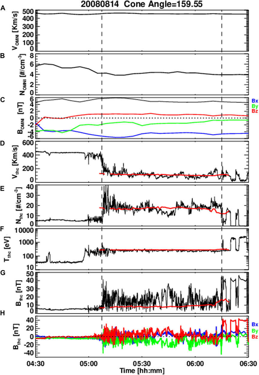
Figure 1. An example of a complete magnetosheath crossing under rIMF conditions recorded by THC and its corresponding upstream conditions from OMNI. From top to bottom: (A) SW speed, (B) SW number density, (C) IMF in GSE coordinates (blue for B_X, green for B_Y, red for B_Z), (D) the proton velocity, (E) proton number density, (F) proton temperature, (G) magnetic magnitude, (H) magnetic field in GSE coordinates, note that the colors stand for same components as in (C). The red lines in panels (D)–(G) are the openGGCM model predictions for each parameter.

The MSH profiles of the magnetic field and plasma parameters of each individual crossing under nIMF or sIMF orientations normalized by their upstream values (OMNI database) are shown in Figure 2 by the gray lines, and red lines stand for medians. A comparison of the left and right panels reveals that the bulk plasma velocity decreases with a distance through MSH under both IMF orientations (Figures 2A, E). The normalized temperature is constant along the whole MSH profile for nIMF (Figure 2B), but it rapidly increases just in front of MP for sIMF (Figure 2F). Since the sIMF results in magnetic reconnection at the subsolar magnetopause, this increase of the temperature is connected with a presence of the boundary layer adjacent to the magnetopause. The normalized N is stable in the first half of MSH and slowly decreases in the region close to MP for nIMF (Figure 2C), but this trend is less distinct for sIMF (Figure 2G). The normalized magnetic field magnitude increases along the path through MSH for both IMF orientations (Figures 2D, H) but the trend is more significant for nIMF (Figure 2D) as the ratio of normalized magnetic field strengths averaged over first and last tenths of the MSH thickness documtents; it is 2.32 for nIMF and 2.08 for sIMF.

Figure 2

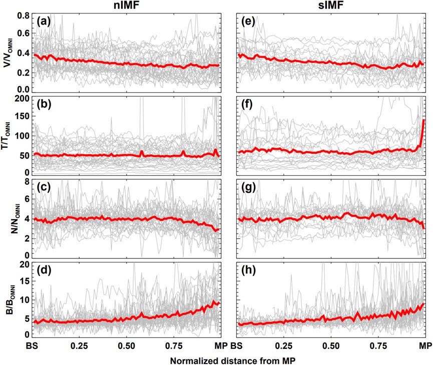
Figure 2. Normalized plasma parameters and magnetic field magnitude for superposed epoch analysis. From (A–H) the proton velocity, proton temperature, proton density, and magnetic field magnitude. (A–D) represents parameters for nIMF, and (E–H) displays them for sIMF.

We have shown that the general trends are similar in both sIMF and nIMF cases—the plasma velocity decreases with distance in MSH, the plasma density and temperature are constant, and the magnetic field increases throughout the MSH. Taking into account a negligible increase of the magnetic field in front of MP for rIMF (Figure 1), we can conclude that the MSH profile under rIMF is more similar to that under the sIMF condition.

Figure 3 shows the median profiles of normalized P_tot and its components in MSH for nIMF (Figure 3A) and sIMF (Figure 3B) orientations. There is a clear decreasing trend of P_tot (black lines) for both IMF orientations, but P_tot at BS is higher under sIMF (1.0 for sIMF and 0.9 for nIMF). Nevertheless, both profiles converge to 0.8 at MP. The decreasing trend is caused by P_d (blue) because P_t (red) is nearly constant (if we ignore the sudden increase of P_t near MP), and P_b (green) increases toward MP; the increasing trend is more rapid for nIMF due to magnetic field pile-up characteristics for this IMF orientation. Nevertheless, P_b in MSH is a minor pressure component with the exception of the close vicinity of MP, where it reaches 30% of the upstream pressure. It is worth noting that the magnitudes of the three pressures are comparable near MP for nIMF, but they are clearly ranked for sIMF (P_t∼0.4, Pd∼0.3, and P_b∼0.1).

Figure 3

Figure 3. The normalized pressures under (A) nIMF and (B) sIMF conditions for the superposed epoch results. The different colors stand for the different pressures.

4.2 Magnetosheath coordinate approach

As noted, we chose the measurements located less than 15° from the Sun-Earth line and in the interval between −0.5 and 1.5 of MSH coordinate, R, and averaged all measurements to 1-min resolution. If the IMF cone angle was lower than 30°, the event was classified as rIMF, and to avoid overlapping of data sets, only events with IMF B_z >2 nT or IMF B_z < −2 nT were considered as nIMF or sIMF, respectively (Šafránková et al., 2009). All measurements were binned into 0.1 R distance bins and normalized to the corresponding upstream observations (propagated Wind observations). Finally, the median values of normalized measurements are used to represent the parameters in a given location. The panels in Figure 4 present (from top to bottom) the normalized values of the plasma velocity V, ion temperature T, number density N, and magnetic field magnitude B with uncertainties; three colors mark IMF orientations, and two dashed vertical lines highlight MP and BS positions. Note that we select the standard error of the mean as a measure of the uncertainties. In our study, the value in each bin is the average of more than hundreds of data points, and thus, the standard error of the mean is rather small, and it often cannot be distinguished in the figures. Hence, we can consider the difference between profiles of MSH parameters presented here as statistically significant.

Figure 4

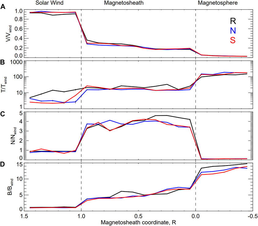
Figure 4. The normalized plasma parameters and magnetic field magnitude as a function of the magnetosheath coordinate. (A) The proton velocity, (B) proton temperature, (C) proton density, and (D) magnetic field magnitude. The colored lines stand for different IMF orientations (red for southward, blue for northward, and black for the radial field). The vertical lines mark the BS (1.0) and MP (0.0) locations.

The majority of results for nIMF (blue) and sIMF (red) in MSH are consistent with the results of a superposed epoch analysis: the velocity profiles are decreasing, the temperature is slightly higher for sIMF near both BS and MP, and the increasing trend of the magnetic field magnitude toward MP is more significant for nIMF. Small-scale features like the decrease in density and temperature increase in front of MP for nIMF are not seen due to the uncertainty of the boundary position in this approach.

The rIMF profiles (black lines) of V are similar to those for the nIMF and sIMF orientations, but the N profile shows a substantial enhancement in the last part of the MSH profile prior to MP. Furthermore, T and B show a decrease and increase trend in different MSH parts.

Although our analysis concentrates on MSH, Figures 4–7 also show normalized profiles of parameters just upstream BS or in the magnetosphere, and we can note preconditioning of the SW in front of BS due to the presence of the foreshock, especially for rIMF. In this respect, one can note a slight decrease in the velocity (Urbar et al., 2019; Xirogiannopoulou et al., 2024) and a rapid increase in the normalized temperature. Upstream temperatures for nIMF and sIMF are by a factor of ∼2 higher than SW temperatures, but it is probably connected with the THEMIS overestimation of the proton temperature (Artemyev et al., 2018).

Figure 5

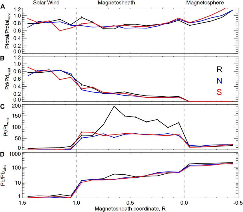
Figure 5. The normalized pressures as a function of the magnetosheath coordinate: (A) the total pressure, Ptotal; (B) Dp; (C) thermal pressure, Pt; and (D) magnetic field pressure, Pb. The color format is the same as in Figure 4.

Figure 6

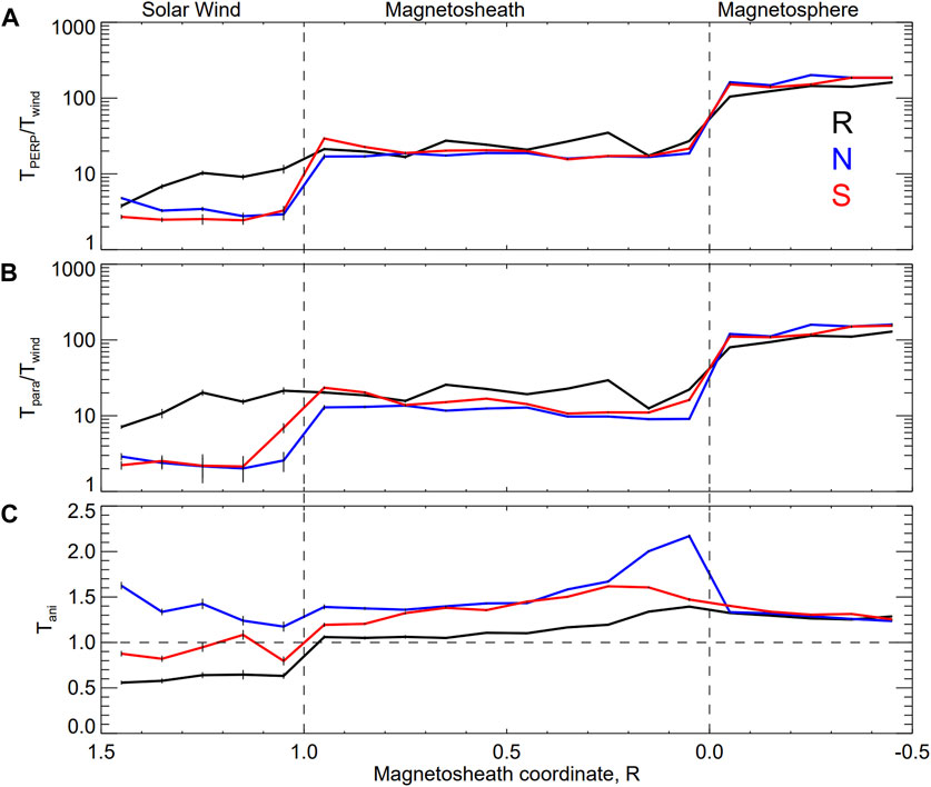
Figure 6. Normalized temperature and T_ANI (T_perp/T_para) as a function of the magnetosheath coordinate: (A) perpendicular temperature, T_perp, (B) parallel temperature, T_para, and (C) T_ANI. The color format is the same as in Figure 4.

Figure 7

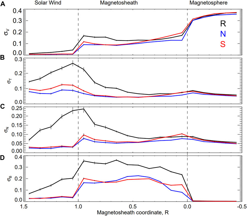
Figure 7. A level of fluctuations as a function of the magnetosheath coordinate. (A) The standard deviation of proton velocity, (B) the standard deviation of proton temperature, (C) the standard deviation of proton density, and (D) the standard deviation of magnetic field magnitude. The color format is the same as in Figure 4.

Figure 5 shows the overview of MSH normalized profiles of individual pressure components for three IMF orientations (the format follows Figure 4). P_tot (Figure 5A) slightly varies around a level of about 0.8 of the upstream pressure, but it does not exhibit pronounced decreasing trend seen in Figure 3, and it is valid for all IMF orientations. P_d follows the decreasing trends for all IMF orientations that correspond to the decreasing trend of the velocity (Figures 2a, 4a). P_t is nearly constant for nIMF and sIMF, but it rapidly increases after the BS crossing for rIMF and its value is significantly larger than for other IMF orientations (Figure 5C). The large value of P_t for rIMF is caused by a combination of the larger N (Figure 4C) and T (Figure 4B, note logarithmic scale in this panel). In the superposed epoch analysis, sIMF exhibits a higher P_t in MSH than in the nIMF case (Figure 3), and it is partly consistent with Figure 5C. A similar increasing trend of P_b (Figure 5D) is observed for all IMF orientations but P_b of rIMF starts to change upstream BS due to foreshock structures. Moreover, P_b in rIMF events exhibits a peak of an unclear origin in the middle of MSH, and such a peak is also seen in the example of the rIMF event in Figure 1.

Since our analysis suggests that foreshock/magnetosheath instabilities can contribute to the overall profile of the average values of magnetic field and plasma parameters in MSH, Figure 6 analyzes profiles of the perpendicular (T_perp) and parallel (T_para) temperatures normalized to their upstream values, as well as temperature anisotropy (T_ANI = T_perp/T_para). The enhanced T_perp and T_para for all IMF orientations in the upstream region are connected with the already mentioned overestimation of the temperature by THEMIS. On the other hand, both T_perp and T_para for rIMF are affected by the reflected particles in the foreshock, and we observe their gradual rise toward MSH values, whereas both components are close to constant prior to the BS crossing for the other two IMF orientations. T_ANI for both sIMF and nIMF orientations are always larger than unity through the whole MSH and increase toward MP with the exception of the boundary layer where T_ANI jumps up for nIMF, whereas a slight decrease can be seen for sIMF. By contrast, the temperature for rIMF is nearly isotropic in the first half of MSH, and an increasing trend of T_ANI is observed in the second half of MSH.

The profiles of T_ANI are consistent with profiles of fluctuation amplitudes shown in Figure 7, presenting the normalized standard deviations of σ_V, σ_T, σ_N, and σ_B, which are used as a measure of the fluctuation level. The standard deviations are calculated in 1-min intervals and normalized by the average upstream SW observations. The foreshock enhances the fluctuation level in front of BS for the rIMF case, and thus, the fluctuation level of all parameters (Figures 7A–D) is higher than that in the other two cases. Also, we observe the highest fluctuation level in MSH for rIMF. A slight increasing trend in MSH of the normalized σ_V for sIMF and nIMF is consistent with the wave generation due to temperature anisotropy. On the other hand, the decrease of the fluctuation level of all plasma parameters (σ_V, σ_T, and σ_N) from BS to the middle of MSH for rIMF is consistent with T_ANI ∼ 1 in this region (Figure 6C). This trend stops at the middle of MSH when T_ANI starts to rise, and its profile is more similar to the profiles of other two IMF orientations.

The rIMF intervals are typically characterized by low N and V (Pi et al., 2014) and, thus, the low pressure exerted on MP. In order to clarify whether a small P_d itself is a proper cause of observed features, Figure 8 highlights the normalized profiles of P_tot and its components for two ranges of upstream P_d. We selected upstream P_d > 2 nPa (red lines) and compared them with P_d < 1 nPa (blue lines) to reveal its influence on other MSH parameters. The figure shows that, besides small dissimilarities like a steeper rise of P_b from BS toward MP for small P_d, the only notable difference is in enhanced normalized P_t through the whole MSH for the low P_d set. However, since this enhancement is lower than that for rIMF (Figure 5C), we can conclude that the proper cause of the enhanced P_t is the larger portion of rIMF events in the low upstream pressure set.

Figure 8

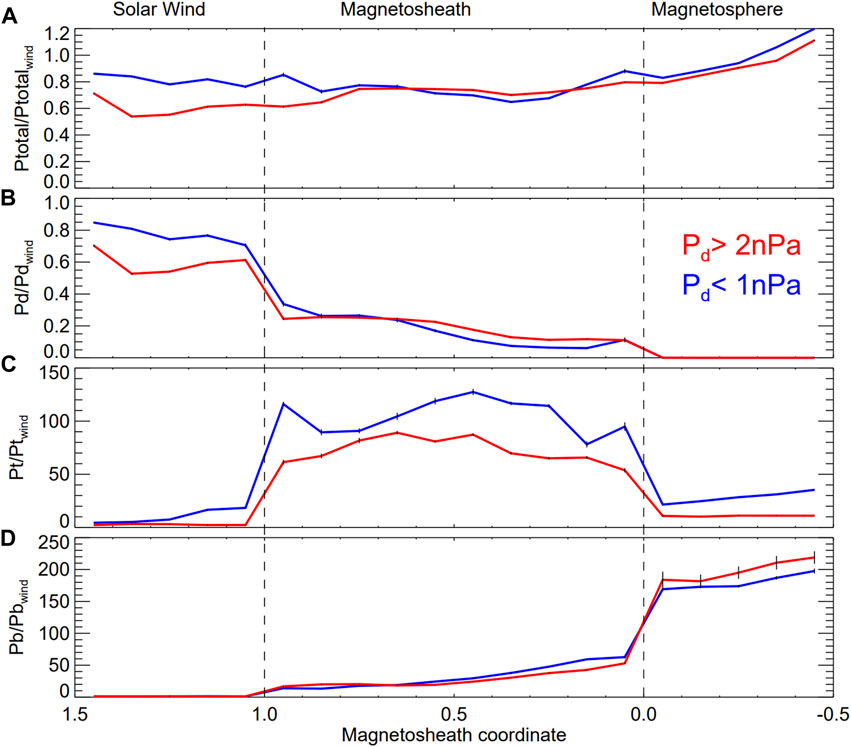
Figure 8. The normalized pressures as a function of the magnetosheath coordinate for two ranges of upstream D_P (red, D_P>2 nPa and blue, D_P<1 nPa): (A) the tota pressure, Ptotal; (B) D_P; (C) thermal pressure, Pt; and (D) magnetic field pressure, Pb.

5 Discussion

This study is devoted to the influence of the IMF direction on the average spatial profiles of magnetic field and plasma parameters across dayside MSH. First, let us clarify the uncertainties affecting this study. It is known that the SW speed changes in a range of 250–800 km/s; the proton density varies from a few units to two hundred cm^-3, and the temperature varies by an order of magnitude. Variations of the IMF magnitude are similar, but the IMF direction can dramatically change in seconds, and all these changes are reflected in MSH. Since the MSH parameters would be related to upstream ones, we use normalized quantities in our analysis. Unfortunately, no near upstream monitor is permanently available, and thus, we use the observations made at the L1 point and propagate them to the spacecraft location (deceleration in MSH is omitted). The propagation routines cannot take into account plasma instabilities modulating SW parameters so that the actual upstream conditions can differ from those predicted. Moreover, Urbar et al. (2019) compared the velocity measured by THEMIS upstream BS with propagated Wind data and found that THEMIS in the magnetospheric mode underestimates the velocity by a factor of 0.93, and it results in ∼15% difference in the dynamic pressure; nevertheless, the difference can be as significant as 30% in individual cases. The inter-calibration, therefore, does not allow us a direct comparison of particular values, but we believe that they cannot change the observed trends. Moreover, the width of the distribution of THEMIS/Wind velocity ratios is about ± 3%, and this uncertainty also contributes to the uncertainty of MP and BS models. The uncertainty of the Shue et al. (1997) model is around 0.8 R_E near the Sun-Earth line (Lin and Wang, 2009), and the Chao et al. (2002) model exhibits an average standard deviation of around 5.7 R_E (e.g., Dmitriev and Chao, 2003). For these reasons, we analyzed the MSH passes using superposed epoch analysis, where the boundaries were certain. This fact allows us to distinguish the MP boundary layers, but this approach still suffers from the uncertainty of estimations of upstream SW parameters. Since the number of MSH passes under a stable IMF orientation is limited, we apply the second approach—a method of the MSH coordinate. However, its results are affected by all aforementioned uncertainties, and it causes relatively huge standard deviations of our average profiles. For example, the average ion speed in MSH is 180.6 km/s with a standard deviation of 97.5 km/s under rIMF conditions.

We use the standard error of the mean as the measure of uncertainty and show it in plots. The number of points used to determine average profiles is large, and the error bars are often hidden within the line thickness. Therefore, we believe that differences between presented profiles are reliable and that they are associated with a particular IMF direction or with a value of the upstream pressure.

As noted, we try to answer three questions from simulation results (Samsonov et al., 2012; Wang et al., 2018):

(1) How does the ratio of upstream to downstream Ptot at BS change with increasing upstream Pd? Specifically, does Ptot decrease significantly after the BS crossing for large Pd (Wang et al., 2018)?

(2) How do the spatial profiles of normalized MSH pressure (P_tot and its components, P_d, P_t, P_b) vary with the IMF orientation with an emphasis on rIMF? In particular, is it roughly constant in the whole MSH profile for nIMF, and does it decreases along the MSH pass for sIMF (Wang et al., 2018) or rIMF (Samsonov et al., 2012)?

(3) What is the role of plasma instabilities in the formation of the MSH spatial profile?

According to the simulation results by Wang et al. (2018) a large upstream pressure cause a decrease in P_tot across BS. This effect is more pronounced for nIMF but still visible for sIMF. However, our analysis (Figure 8) shows different results. The low THEMIS P_d in the upstream was already discussed and attributed to an underestimation of the ion velocity, but it would not affect the overall profiles. Nevertheless, Figure 8 shows that P_tot is maintained from the solar wind toward MP if the upstream P_d is low, and even P_tot increase in the BS vicinity is observed for higher P_d. The low MSH P_tot in the model is probably connected with an underestimation of MSH P_t that compensates the decrease of P_d. We cannot compare this feature with our analysis because it combines all IMF orientations, and thus, the higher P_t in the P_d<1 nPa set is probably connected with an enhanced portion of rIMF events in this set (Pi et al., 2014).

The influence of the IMF orientation on the pressure profiles in MSH was investigated in two ways, and their results are almost consistent (Figures 3, 5); the differences near MSH boundaries are connected with the problem of their determination in the MSH coordinate approach. The Wang et al. (2018) simulations predict constant P_tot across MSH for nIMF and its decrease toward MP for sIMF, but we do not see any notable difference between these two IMF orientations. The P_t profile in simulations rises toward MP and exhibits a bump in the MSH center for nIMF, but it is flat for all IMF orientations in observations. A much larger P_t for rIMF than for the other two orientations is consistent with calculations by Samsonov et al. (2012), but these calculations predict a gradual rise of P_t toward MP, but a decrease is observed in Figure 5C.

Figure 5 shows the distribution of P_tot and its components along the path from the SW to the magnetosphere. As could be expected, the whole system is in the pressure equilibrium because an increase in P_t and P_b for all IMF orientations balances a decrease in P_d. The only notable feature is the excess of normalized P_t for rIMF in MSH due to an increased temperature and a density peak in front of MP (Figure 4). This increase of P_t can also be related to T_ANI changes under rIMF conditions. As the V decreases, an increasing N is expected, but they are absent for nIMF and sIMF. It can be related to the draped magnetic field lines increasing the magnetic field strength, pushing the plasma away, and creating a depletion layer for nIMF. Note that subsolar reconnection also moves the solar wind flux away for sIMF.

P_d for rIMF shows a smooth change when it crosses BS. We suggest that it is related to BS non-stationarity. The simulations of the BS formation by De Stretck and Poedts (1999) reveal that BS under a field-aligned flow is an unstable structure. They conclude that the intermediate BS could form under rIMF conditions. Lin and Wang (2005) also performed a 3D simulation of BS under rIMF. Their results show that the quasi-parallel BS is nonstationary and its reformation frequently occurs. Both studies imply that BS is unstable under rIMF, and this can result in the non-sharp BS crossing in our statistics.

In order to elucidate the possible sources of differences between models and observations, we have investigated the role of fluctuations in the formation of the mean MSH profiles. The foreshock effect is a general phenomenon that can be noticed in our results because the foreshock can be found in front of BS under all IMF orientations and covers the whole dayside BS under rIMF conditions. The high fluctuation level of all parameters (Figure 7) in front of BS increases the temperature (Figure 4B) for rIMF. Figure 6C shows that T_ANI under rIMF is ∼0.5 in the foreshock region and becomes ∼1 in the first-half MSH, but Pi et al. (2022) report that T_ANI is close to 1 in SW for the rIMF events. The reason for the T_ANI decrease is the increasing T_PARA (Figure 6B) by the reflected particles in the foreshock. T_ANI jumps to around 1 in MSH for rIMF, and it is consistent with the finding of Czaykowska et al. (2000) that quasi-parallel BS is less effective in increasing T_ANI than quasi-perpendicular BS. The simulation results of Samsonov et al. (2012) also imply that T_ANI in MSH is ∼1 for rIMF (see Figure 2 in that paper). Large MSH T_ANI for nIMF and sIMF orientations maintain the level of fluctuations of all parameters through the whole MSH but nearly isotropic temperature for rIMF in the first half of MSH leads to their damping. As a result, there are no noticeable differences in fluctuation levels between different IMF orientations just in front of MP, with the exception of the magnetic field.

6 Conclusion

We used two methods to investigate the SW modification in MSH for different IMF orientations. The first approach is based on the superposed epoch analysis of complete MSH crossings recorded by THB and THC during 2007–2010. The second method applies the radial distance of the spacecraft from the model MP normalized to the MSH thickness for all THEMIS observations in the subsolar MSH. We should note that the results of both approach analyses are generally consistent, regardless of the fact that we encountered some of the above-mentioned differences.

Applications of our two analyses allow us to summarize the results as follows:

(1) We did not find any influence on the value of the upstream pressure on the mean magnetosheath profile.

(2) The sign of the IMF north-south component has a negligible effect on the spatial profile of the magnetic field strength or plasma parameters as well as on the level of fluctuations;

(3) Radially pointing IMF does not change the profiles of the magnetic field strength, ion velocity, or ion density, but the temperature is enhanced by a factor of 2 through MSH;

(4) The temperature anisotropy, T_ANI, in MSH with the exception of the MP boundary layer is approximately 1.4 for nIMF and sIMF, but it is close to unity for rIMF;

(5) The fluctuation level of plasma parameters just downstream BS is enhanced under a radial IMF, but it gradually decreases toward MP to a value typical for other IMF orientations;

(6) When IMF points radially, the magnetic field fluctuations in the whole MSH are enhanced by a factor of 1.7.

All these features are associated with the preconditioning of the SW plasma and IMF in the foreshock that is present under rIMF but missing during the other IMF orientations.

Since we did not confirm the suggestions following from models (Samsonov et al., 2012; Wang et al., 2018), we plan to use the collected data for a complex comparison with local magnetosheath models like Vandas et al. (2020) in the near future.

Data availability statement

Publicly available datasets were analyzed in this study. This data can be found here: https://cdaweb.gsfc.nasa.gov/.

Author contributions

GP: Conceptualization, Data curation, Formal Analysis, Investigation, Methodology, Visualization, Writing–original draft, Writing–review and editing. ZN: Formal Analysis, Investigation, Supervision, Validation, Writing–review and editing. JŠ: Funding acquisition, Investigation, Methodology, Writing–review and editing. KG: Methodology, Writing–review and editing.

Funding

The author(s) declare that financial support was received for the research, authorship, and/or publication of this article. This work was supported by the Czech Science Foundation under project 21-26463S.

Acknowledgments

The authors thank Prof. Vitek for his helpful comments during late-night meetings.

Conflict of interest

The authors declare that the research was conducted in the absence of any commercial or financial relationships that could be construed as a potential conflict of interest.

Publisher’s note

All claims expressed in this article are solely those of the authors and do not necessarily represent those of their affiliated organizations, or those of the publisher, the editors and the reviewers. Any product that may be evaluated in this article, or claim that may be made by its manufacturer, is not guaranteed or endorsed by the publisher.

References

Anderson, B. J., and Fuselier, S. A. (1993). Magnetic pulsations from 0.1 to 4.0 Hz and associated plasma properties in the Earth's subsolar magnetosheath and plasma depletion layer. J. Geophys. Res. 98, 1461–1479. doi:10.1029/92JA02197

CrossRef Full Text | Google Scholar

Artemyev, A. V., Angelopoulos, V., and McTiernan, J. M. (2018). Near-Earth solar wind: plasma characteristics from ARTEMIS measurements. J. Geophys. Res. Space Phys. 123, 9955–9962. doi:10.1029/2018JA025904

CrossRef Full Text | Google Scholar

Auster, H. U., Glassmeier, K. H., Magnes, W., Aydogar, O., Baumjohann, W., Constantinescu, D., et al. (2008). The THEMIS fluxgate magnetometer. Space Sci. Rev. 141, 235–264. doi:10.1007/s11214-008-9365-9

CrossRef Full Text | Google Scholar

Bieber, J. W., and Stone, S. C. (1979). “Energetic electron bursts in the magnetopause electron layer and in interplanetary space,” in Magnetospheric Boundary layers. Editors B. Battrick, J. Mort, and G. Haerendel (Neuilly, France: Eur. Space Agency Spec. Publ.), 131–135. ESA SP-148.

Google Scholar

Blanco-Cano, X., Omidi, N., and Russell, C. T. (2009). Global hybrid simulations: foreshock waves and cavitons under radial interplanetary magnetic field geometry. J. Geophys. Res. 114 (A1). doi:10.1029/2008JA013406

CrossRef Full Text | Google Scholar

Chao, J. K., Wu, D. J., Lin, H.-H., Yang, Y.-H., Kessel, M., Chen, S. H., et al. (2002). Models for the size and shape of the earth’s magnetopause and bow shock. COSPAR Colloq. Ser. 12 (C), 127–135. doi:10.1016/S0964-2749(02)80212-8

CrossRef Full Text | Google Scholar

Czaykowska, A., Bauer, T. M., Treumann, R. A., and Baumjohann, W. (2000) Average observed properties of the Earth's quasi-perpendicular and quasi-parallel bow shock. arXiv: physics/0009046v1.

Google Scholar

De Sterck, H., and Poedts, S. (1999). Field-aligned magnetohydrodynamic bow shock flows in the switch-on regime. Astron. Astrophys. 343, 641–649.

Google Scholar

Dimmock, A. P., and Nykyri, K. (2013). The statistical mapping of magnetosheath plasma properties based on THEMIS measurements in the magnetosheath interplanetary medium reference frame. J. Geophys. Res. 118, 4963–4976. doi:10.1002/jgra.50465

CrossRef Full Text | Google Scholar

Dmitriev, A. V., Chao, J.-k., and Wu, D. J. (2003). Comparative study of bow shock models using Wind and Geotail observations. J. Geophys. Res. 108, A12,1464. doi:10.1029/2003JA010027

CrossRef Full Text | Google Scholar

Gary, S. P., McKean, M. E., and Winske, D. (1993). Ion cyclotron anisotropy instabilities in the magnetosheath: theory and simulations. J. Geophys. Res. 98, 3963–3971. doi:10.1029/92JA02585

CrossRef Full Text | Google Scholar

Jelínek, K., Němeček, Z., and Šafránková, J. (2012). A new approach to magnetopause and bow shock modeling based on automated region, identification. J. Geophys. Res. 117, A05208. doi:10.1029/2011JA017252

CrossRef Full Text | Google Scholar

Jung, J., Connor, H., Dimmock, A., Sembay, S., Read, A., and Soucek, J. (2024). Mshpy23: a user-friendly, parameterized model of magnetosheath conditions. Earth Planet. Phys. 8 (1), 89–104. doi:10.26464/epp2023065

CrossRef Full Text | Google Scholar

Lin, Y., and Wang, X. Y. (2005). Three-dimensional global hybrid simulation of dayside dynamics associated with the quasi-parallel bow shock. J. Geophys. Res. 110, A12216. doi:10.1029/2005JA011243

CrossRef Full Text | Google Scholar

Liu, Z.-Q., Lu, J. Y., Wang, C., Kabin, K., Zhao, J. S., Wang, M., et al. (2015). A three-dimensional high Mach number asymmetric magnetopause model from global MHD simulation. J. Geophys. Res. Space Phys. 120, 5645–5666. doi:10.1002/2014JA020961

CrossRef Full Text | Google Scholar

Longmore, M., Schwartz, S. J., Geach, J., Cooling, B. M. A., Dandouras, I., Lucek, E. A., et al. (2005). Dawn-dusk asymmetries and sub-Alfvénic flow in the high and low latitude magnetosheath. Ann. Geophys. 23, 3351–3364. doi:10.5194/angeo-23-3351-2005

CrossRef Full Text | Google Scholar

Ma, X., Nykyri, K., Dimmock, A., and Chu, C. (2020). Statistical study of solar wind, magnetosheath, and magnetotail plasma and field properties: 12+ years of THEMIS observations and MHD simulations. J. Geophys. Res. Space Phys. 125, e2020JA028209. doi:10.1029/2020JA028209

CrossRef Full Text | Google Scholar

McFadden, J. P., Carlson, C. W., Larson, D., Bonnell, J., Mozer, F. S., Angelopoulos, V., et al. (2008). The THEMIS ESA plasma instrument and in-flight calibration. Space Sci. Rev. 141, 277–302. doi:10.1007/s11214-008-9440-2

CrossRef Full Text | Google Scholar

Midgley, J. E., and Davis, L. (1963). Calculation by a moment technique of the perturbation of the geomagnetic field by the solar wind. J. Geophys. Res. 68, 5111–5123. doi:10.1029/JZ068i018p05111

CrossRef Full Text | Google Scholar

Němeček, Z., Šafránková, J., Grygorov, K., Mokrý, A., Pi, G., Aghabozorgi Nafchi, M., et al. (2023). Extremely distant magnetopause locations caused by magnetosheath jets. Geophys. Res. Lett. 50 (24), e2023GL106131. Art. No. doi:10.1029/2023GL106131

CrossRef Full Text | Google Scholar

Němeček, Z., Šafránková, J., Kruparova, O., Přech, L., Jelínek, K., Dušík, Š., et al. (2015). Analysis of temperature versus density plots and their relation to the LLBL formation under southward and northward IMF orientations. J. Geophys. Res. Space Phys. 120, 3475–3488. doi:10.1002/2014JA020308

CrossRef Full Text | Google Scholar

Němeček, Z., Šafránková, J., Zastenker, G. N., Pisoft, P., and Jelínek, K. (2002). Low-frequency variations of the ion flux in the magnetosheath. Planet. Space Sci. 50 (5-6), 567–575. doi:10.1016/S0032-0633(02)00036-3

CrossRef Full Text | Google Scholar

Němeček, Z., Šafránková, J., Zastenker, G. N., Pišoft, P., Paularena, K. I., and Richardson, J. D. (2000). Observations of the radial magnetosheath profile and a comparison with gasdynamic model predictions. Geophys. Res. Lett. 27, 2801–2804. doi:10.1029/2000GL000063

CrossRef Full Text | Google Scholar

Paularena, K. I., Richardson, J. D., Kolpak, M. A., Jackson, C. R., and Siscoe, G. L. (2001). A dawn-dusk density asymmetry in Earth’s magnetosheath. J. Geophys. Res. 106 (A11), 25377–25394. doi:10.1029/2000ja000177

CrossRef Full Text | Google Scholar

Pi, G., Němeček, Z., Šafránková, J., Grygorov, K., and Shue, J.-H. (2018). Formation of the dayside magnetopause and its boundary layers under the radial IMF. J. Geophys. Res. Space Phys. 123, 3533–3547. doi:10.1029/2018JA025199

CrossRef Full Text | Google Scholar

Pi, G., Pitňa, A., Zhao, G.-Q., Němeček, Z., Šafránková, J., and Tsai, T.-C. (2022). Properties of magnetic field fluctuations in long-lasting radial IMF events from wind observation. Atmosphere 13, 173. doi:10.3390/atmos13020173

CrossRef Full Text | Google Scholar

Pi, G., Shue, J.-H., Chao, J.-K., Němeček, Z., Šafránková, J., and Lin, C.-H. (2014). A reexamination of long-duration radial IMF events. J. Geophys. Res. Space Phys. 119, 7005–7011. doi:10.1002/2014JA019993

CrossRef Full Text | Google Scholar

Pi, G., Shue, J.-H., Grygorov, K., Li, H.-M., Němeček, Z., Šafránková, J., et al. (2017). Evolution of the magnetic field structure outside the magnetopause under radial IMF conditions. J. Geophys. Res. Space Phys. 122, 4051–4063. doi:10.1002/2015JA021809

CrossRef Full Text | Google Scholar

Pi, G., Shue, J.-H., Park, J.-S., Chao, J.-K., Yang, Y.-H., and Lin, C.-H. (2016). A comparison of the IMF structure and the magnetic field in the magnetosheath under the radial IMF conditions. Adv. Space Res. 58 (2), 181–187. doi:10.1016/j.asr.2015.11.012

CrossRef Full Text | Google Scholar

Šafránková, J., Goncharov, O., Němeček, Z., Přech, L., and Sibeck, D. G. (2012). Asymmetric magnetosphere deformation driven by hot flow anomaly(ies). Geophys. Res. Lett. 39 (15). Art. No. L15107. doi:10.1029/2012GL052636

CrossRef Full Text | Google Scholar

Šafránková, J., Hayosh, M., Gutynska, O., Němeček, Z., and Přech, L. (2009). Reliability of prediction of the magnetosheath B_<i>Z</i> component from interplanetary magnetic field observations. J. Geophys. Res. Space Phys. 114, A12213. doi:10.1029/2009JA014552

CrossRef Full Text | Google Scholar

Šafránková, J., Němeček, Z., Dušík, Š., Přech, L., Sibeck, D. G., and Borodkova, N. N. (2002). The magnetopause shape and location: a comparison of the Interball and Geotail observations with models. Ann. Geophys. 20 (3), 301–309. doi:10.5194/angeo-20-301-2002

CrossRef Full Text | Google Scholar

Samsonov, A. A., Němeček, Z., Šafránková, J., and Jelínek, K. (2012). Why does the subsolar magnetopause move sunward for radial interplanetary magnetic field? J. Geophys. Res. Space Phys. 117, A5. doi:10.1029/2011JA017429

CrossRef Full Text | Google Scholar

Shue, J.-H., Chao, J. K., Fu, H. C., Russell, C. T., Song, P., Khurana, K. K., et al. (1997). A new functional form to study the solar wind control of the magnetopause size and shape. J. Geophys. Res. 102 (A5), 9497–9511. doi:10.1029/97JA00196

CrossRef Full Text | Google Scholar

Sibeck, D. G., and Angelopoulos, V. (2008). THEMIS science objectives and mission phases. Space Sci. Rev. 141, 35–59. doi:10.1007/s11214-008-9393-5

CrossRef Full Text | Google Scholar

Spreiter, J. R., and Stahara, S. S. (1980). A new predictive model for determining solar wind-terrestrial planet interactions. J. Geophys. Res. 85, 6769–6777. doi:10.1029/JA085iA12p06769

CrossRef Full Text | Google Scholar

Spreiter, J. R., Summers, A. L., and Alksne, A. Y. (1966). Hydromagnetic flow around the magnetosphere. Planet. Space Sci. 14, 223–253. doi:10.1016/0032-0633(66)90124-3

CrossRef Full Text | Google Scholar

Urbář, J., Němeček, Z., Šafránková, J., and Přech, L. (2019). Solar wind proton deceleration in front of the terrestrial bow shock. J. Geophys. Res. Space Phys. 124 (8), 6553–6565. doi:10.1029/2019JA026734

CrossRef Full Text | Google Scholar

Vandas, M., Němeček, Z., Šafránková, J., Romashets, E. P., and Hajoš, M. (2020). Comparison of observed and modeled magnetic fields in the Earth's magnetosheath. J. Geophys. Res. Space Phys. 125 (3), e2019JA027705. doi:10.1029/2019JA027705

CrossRef Full Text | Google Scholar

Wang, J., Guo, Z., Ge, Y. S., Du, A., Huang, C., and Qin, P. (2018). The responses of the earth’s magnetopause and bow shock to the IMF Bz and the solar wind dynamic pressure: a parametric study using the AMR-CESE-MHD model. J. Space Weather Space Clim. 68, A41. doi:10.1051/swsc/2018030

CrossRef Full Text | Google Scholar

Wang, M., Lu, J. Y., Kabin, K., Yuan, H. Z., Zhou, Y., and Guan, H. Y. (2020). Influence of the interplanetary magnetic field cone angle on the geometry of bow shocks. Astrophys. J. 159, 227. doi:10.3847/1538-3881/ab86a7

CrossRef Full Text | Google Scholar

Xirogiannopoulou, N., Goncharov, O., Šafránková, J., and Němeček, Z. (2024). Characteristics of foreshock subsolar compressive structures. J. Geophys. Res. 129 (2). Art. No. e2023JA032033. doi:10.1029/2023JA032033

CrossRef Full Text | Google Scholar

Zastenker, G. N., Nozdrachev, M. N., Němeček, Z., Šafránková, J., Paularena, K. I., Richardson, J. D., et al. (2002). Multispacecraft measurements of plasma and magnetic field variations in the magnetosheath: comparison with Spreiter models and motion of the structures. Planet. Space Sci. 50 (5-6), 601–612. doi:10.1016/S0032-0633(02)00039-9

CrossRef Full Text | Google Scholar

Zhang, H., Fu, S., Pu, Z., Lu, J., Zhong, J., Zhu, C., et al. (2019). Statistics on the magnetosheath properties related to magnetopause magnetic reconnection. Astrophys. J. 880, 122. doi:10.3847/1538-4357/ab290e

CrossRef Full Text | Google Scholar

Zhang, H., Zong, Q., Connor, H., Delamere, P., Facskó, G., Han, D., et al. (2022). Dayside transient phenomena and their impact on the magnetosphere and ionosphere. Space Sci. Rev. 218, 40. doi:10.1007/s11214-021-00865-0

PubMed Abstract | CrossRef Full Text | Google Scholar