Evidence of Kelvin-Helmholtz and tearing mode instabilities at the magnetopause during space weather events

Introduction: Kelvin-Helmholtz (KH) and tearing mode (TM) instabilities are one of the most important mechanisms of solar wind energy, momentum and plasma transport within the magnetosphere.

Methods: To investigate the conditions under which KHTM instabilities occur in the Earth environment it is fundamental to combine simultaneous multipoint in situ measurements and MHD simulations. We analyzed data from the THEMIS and Cluster spacecraft considering two Space Weather (SWE) events starting with an M2.0 flare event (hereafter Case-1) that occurred on 21 June 2015 and the most-intensive flare (X9.3) of solar cycle 24 that occurred on 6 September 2017 (hereafter Case-2).

Results: Our analysis utilized a 2D MHD model for incompressible and viscous flow. The results from Case-1 indicate the presence of KH and TM instabilities, suggesting existence of observed low-amplitude oscillations at the nose of the magnetopause. However, the MHD simulations for Case-2 did not show any evidence of KH vortices, but did reveal the presence of “magnetic island” structures during a low-shear condition. The reconnection rate derived from the observations is compared with the computed one in the presence of developed instabilities inside the Earth’s magnetopause.

1 Introduction

Kelvin-Helmholtz instability (Axford and Hines, 1961) (KHI) is an ubiquitous phenomenon that occurs in several distinct environments: from oceans (e.g., Mahony, 1977; Smyth and Moum, 2012) to clouds (e.g., Houze, 2014; Cann et al., 2022) on Earth, from diffusive nebulae (e.g., Orion Nebula, Berné et al., 2010; Berné and Matsumoto, 2012; Yaghouti et al., 2017) to the internal structure of relativistic outflows (e.g., the jet in 3C 273, Lobanov and Zensus, 2001; Perucho et al., 2006). KHI is considered one of the main processes of transferring solar wind energy, momentum and plasma inside magnetosphere (Kivelson and Chen, 1995; Chen et al., 1997; Fairfield et al., 2000; Hasegawa et al., 2004). At the Earth, KHIs are observable in the form of waves (KHWs) within the magnetopause region between the anti-Sunward magnetosheath and the relatively stagnant magnetosphere. The onset of KHI is influenced by the interplay between the stabilizing effects of compressibility and magnetic tension force (Masson and Nykyri, 2018) and the destabilizing effects arising from velocity shear produced by the magnetosphere and the magnetosheath. This shear creates a difference in momentum, leading to an unstable condition, that provides the energy required to initiate and eventually further sustain the instability. When the velocity shear exceeds the magnetic energy, it destabilizes the magnetopause boundary and enables the development of Kelvin-Helmholtz waves into nonlinear rolled-up vortices (KHVs) (Hwang et al., 2022). Analysing 7 years of in situ data collected by the NASA THEMIS mission, Kavosi and Raeder (2015) found that KHWs occur at the (flank) magnetopause for approximately 19% of that time. The occurrence of these waves is influenced by factors such as solar wind speed, Alfven Mach number and number density, and is mostly independent on the IMF magnitude. These conditions can be easily met when a perturbation propagates within the interplanetary medium, such as during the occurrence of a coronal mass ejection. KHIs have also been observed in other planetary systems either when they possess a magnetic field, such as Mercury (e.g., Sundberg et al., 2010; Liljeblad et al., 2014) and Saturn (e.g., Masters et al., 2010; Delamere et al., 2013), or in planets that lack an intrinsic magnetic field, such as Venus (e.g., Amerstorfer et al., 2007; Pope et al., 2009).

The dominant process that governs the solar wind plasma entry in the magnetosphere is magnetic reconnection (MR, Dungey, 1961), both at the magnetopause dayside (Trattner et al., 2021) and at the magnetotail nightside (Øieroset et al., 2001). This mechanism takes place in a diffusion region centred around a magnetic X-line, where magnetic field lines of opposite polarity interact, break, and then reconnect in a different configuration (Øieroset et al., 2001). Both KHI and MR facilitate the transport of plasma in the magnetosphere-ionosphere system but differ in various aspects. Firstly, KHI typically occurs at both duskward and dawnward flanks of the magnetopause, whereas MR is less likely to take place in these regions. Secondly, the occurrence of MR at the sub-solar magnetopause is closely connected with the IMF orientation at the planetary magnetosphere. At Earth, MR is favoured when the IMF is directed southward (Kavosi and Raeder, 2015; Masson and Nykyri, 2018), because the planetary magnetic field has opposite direction. When the IMF is northward, MR becomes less favoured but could occur through several distinct mechanisms, such as the (i) merging of magnetosheath magnetic field lines and (ii) opening (lobe) of magnetic field lines poleward of the cusps (for detailed description see Fuselier et al., 2018). In contrast to MR, KHIs could develop regardless of the IMF direction. However, recent works about the Earth’s and Mercury’s magnetospheres show that KHWs are much less frequent when the IMF is southward, because (i) MR and flux transfer events disrupt the development of vortex structures (Hwang et al., 2011; Sundberg et al., 2012; Hwang et al., 2022) and (ii) when the magnetic field is aligned with the plasma flow, the field tension is minimized by northward IMF (Chandrasekhar, 1961; Sundberg et al., 2012).

Over the past few decades, several missions have been launched to investigate the dynamics of the circumterrestrial environment aiming to answering unresolved questions on magnetopause dynamics related, for instance, to the occurrence rate of KHIs and their evolution into rolled-up vortices, the asymmetry between dawnward and duskward regions, and whether MR could occur inside rolled-up vortices or via their interaction (for more details see Masson and Nykyri, 2018). Missions such as THEMIS (Angelopoulos, 2008), Cluster (Escoubet et al., 2001) and MMS (Burch et al., 2016) have contributed significantly to our understanding of KHI. Based on data from these missions, several important findings have emerged: (i) KHIs are a common phenomenon (Hasegawa et al., 2004; 2006), (ii) KHIs can be generated under different IMF conditions (Hasegawa et al., 2006; Liljeblad et al., 2014), (iii) KHIs can lead to rolled-up vortices (Lin et al., 2014; Hwang et al., 2020), (iv) KHVs drive the onset of magnetic reconnection (Vortex-Induced Reconnection, VIR) leading to development of Tearing Mode instability (Chen et al., 1997) and formation of magnetic islands, evolving into flux ropes (Eriksson et al., 2009; Nakamura et al., 2013), and (v) in the late nonlinear phase, vortex merging and secondary KHIs development in a wider latitudinal range (Sisti et al., 2019).

The phenomenon of KHI gives rise to the formation of KHWs. The latter can be classified as linear or non-linear waves based on their association with a mixing region. Non-linear KHWs produce KHVs, that are distinguishable during spacecraft transitions through their leading and trailing edges (e.g., Vernisse et al., 2016; Settino et al., 2022). The rolled-up vortices are characterised by sawtooth signatures in IMF (e.g., Figure 6 in Fairfield et al., 2007; Hasegawa et al., 2009; Sundberg et al., 2012) and by the density reversal signatures in plasma data (e.g., Figure 2 in Hasegawa et al., 2004; Hwang et al., 2022). KHVs can provide favourable conditions for MR, driving transient magnetic structures at the dayside magnetopause, i. e., flux-transfer events (FTEs, Fear et al., 2008). FTEs transfer magnetic flux and plasma within the magnetosphere, leading to a temporary restructuring of the magnetic field lines. This process influences the evolution of KHVs dampening their spatial evolution. Contrary, the linear KHWs exhibit a box-like pattern in observations, that represents an abrupt transition from the more-turbulent magnetosheath to the more-stable magnetosphere. This transition is characterised by (i) reduced B_z, (ii) more flux of low-energy ions ($<$ 1 keV), (iii) enhanced anti-sunward flow velocity v_x and (iv) ion density (Hwang et al., 2022). Note that the linear KHWs do not trigger MR, thus, preventing the transfer of energy and plasma through the magnetopause.

In the last years, several works (e.g., Hasegawa et al., 2004; Fairfield et al., 2007; Hasegawa et al., 2009; Vernisse et al., 2016; Masson and Nykyri, 2018; Hwang et al., 2022; Settino et al., 2022) have analysed observations of terrestrial KHWs and have established three criteria for identifying them (Liljeblad et al., 2014), as summarized as follows:

• quasi-periodicity of waves;

• presence of magnetospheric and magnetosheath signatures during each wave period;

• absence of active processes in the magnetopause, such as the flux transfer events and either ion cyclotron, or mirror waves. The presence of alternative processes could potentially interfere with or obscure the identification of Kelvin-Helmholtz waves. Ensuring the absence of these specific processes enhances our confidence in attributing observed magnetic field fluctuations to KHW. Essentially, this criterion practically helps isolating and identifying KHWs.

All these criteria are utilised to identify the development of KHWs. In this study, we performed data analysis for two distinct events, according to the fulfillment of these criteria. Model-based investigations can be conducted to confirm the development of KHIs.

The study and interpretation of the KHIs have been carried out using various magnetohydrodynamic (MHD) models (e.g., PLUTO, BATS-R-US, Mignone et al., 2007; Powell et al., 1999) that can be categorized according to their complexity. The simplest single-fluid models solve the set of coupled equations that describe the behaviour of magnetised plasma, including the conservation of mass, momentum, energy, and Maxwell’s equations. More complex two-fluid simulation MHD models (e.g., Sisti et al., 2019) play a significant role in interpreting and simulating KHIs. These simulations provide information about the growth, evolution, and characteristics of KHIs, such as the formation of vortices, mixing of plasma, and energy dissipation. In this work, we take advantage of a MHD model for incompressible, viscous and electrically-conductive flow presented by Ivanovski et al. (2011). The code uses a flexible numerical scheme that allows to simulate the 2D coupled KH and TM instabilities.

This paper is organised as follows. Section 2 focuses on two specific cases: a solar eruption on 21 June 2015 and one on 6 September 2017. In both cases the related interplanetary (IP) shock compressed the magnetopause earthward at about 5 Earth radii (R_⊕). In Case-1, the THEMIS and Cluster spacecraft constellations crossed the stable magnetopause at their minimum distance from the Earth. In Case-2, THEMIS, Cluster and MMS encountered the magnetopause during its abrupt transition toward and outward the Earth. In Section 3 we present our MHD model. In Section 4.1 and 4.2 we show the results of the simulations for Case-1 and Case-2, respectively. We also report the reconnection rates derived from spacecraft data with those obtained from the MHD simulations. We compare the results against the observational data collected by the aforementioned spacecraft and in Section 5 we summarize our findings.

2 21 June 2015 and 6 September 2017 events

In this work, the Space Weather events starting on 21 June 2015 (Case-1) and on 6 September 2017 (Case-2) have been studied, as intended in Laurenza et al. (2023). In both cases an intense flare and halo-CME were produced but the geomagnetic effects were different. In Case-1, the halo-CME headed to Earth and led to a major geomagnetic storm (Dst = −204 nT, Joshi et al., 2018), whereas the halo-CME generated by Case-2 produced a less intense storm (Dst = −124 nT, Bruno et al., 2019) because the CME is not directed to Earth and, therefore, only the lateral part of the CME reached the Earth.

2.1 Case-1: the 21–22 June 2015 event

On 21 June 2015 two distinct flares of class M2.0 (2015-06-21T01:02:00-FLR-001) and M2.6 (2015-06-21T02:06:00-FLR-001) erupted from the same active region (AR 12371) located at the heliospheric position N13E23. The Solar Dynamics Observatory (SDO, Pesnell et al., 2012) provides a visual representation of the event through a series of images captured from 01:26 to 03:11 UT (Supplementary Figure S3). This sequence clearly shows that the evolution between the two events occurred without interruption, suggesting a unique continuous event, as indicated in Piersanti et al. (2017). Also Joshi et al. (2018) investigated the AR during the first and second flares, identifying a two-step eruption process of a magnetic flux rope, that resulted in two consecutive flares. More in detail, the flux rope eruption proceeded in a distinct direction in the two phases. Nevertheless, hereafter we indicate the event as unique instead of two distinguished events, as indicated in Piersanti et al. (2017).

This event triggered the development of a CME flux rope, as highlighted by the post-eruptive arcades (Tripathi et al., 2004). Images of a CME expansion through the heliosphere were retrieved by the SOHO/LASCO coronographs (Brueckner et al., 1995), whose fields-of-view (FoVs) span 2–6 R_⊙ (LASCO-C2) and 3.7–32 R_⊙ (LASCO-C3) (see Supplementary Figure S4). More specifically, a halo-CME can be observed moving towards the spacecraft within its FoV. Moreover, a shock-front is visible ahead of the CME. The resulting velocity measurements indicated $\bar{v}\sim$ 1,400 km s⁻¹ and retrieved an acceleration a ∼ 21 m s⁻² at a height of 20 R_⊙. On the whole, during the early phase the halo-CME slightly accelerated (a ∼ 100 m s⁻²), whereas it decelerated (a ∼ − 200 m s⁻²) during the successive expansion.

The resulting interplanetary coronal mass ejection (ICME), produced an IP shock that arrived at Earth at 17:59 UT on 22 June 2015. The developed ICME magnetic sheath region and the magnetic cloud (MC) were identified by the ACE spacecraft (see Supplementary Figure S5). On one hand, the magnetic sheath region was characterised by enhanced plasma density (nearly 40 p cm⁻³) and by magnetic field turbulence, which led to abrupt oscillations. On the other hand, the MC was located about 8 h after the shock wave. Distinct features marked its passage both on the magnetic field (e.g., the coherent smooth oscillation of the magnetic field components or smooth increase of B_z) and plasma data. Then, the smooth speed decrease from the ICME front (∼750 km s⁻¹) to the back (∼600 km s⁻¹) suggests that the MC was expanding.

Energetic Storm Particles (ESPs) events, i.e., local increases of energetic charged particle intensities can be observed at IP shocks (Chiappetta et al., 2021, and references therein). The arrival of the IP shock produced an enhancement in the proton intensities of ∼ 1 order of magnitude in all energy channels.

The Case-1 event led to a major geomagnetic storm on 23 June 2015. Specifically, immediately after the IP shock two abrupt changes of the Dst and K_p indices were noted: the first one, at 21:00 UT Dst= −114 nT and K_p= 8+ evidences the intense storm regime; and the second one, nearly 12 h later, evidences ∼ intense (Dst = −198 nT, 2 times more intense than the first one) and severe storm (K_p = 8-) regimes. The evolution of the geomagnetic storm suggests the presence of a double storm, associated with periods when the z-component of IMF was negative. Piersanti et al. (2017) attributed the first period to the arrival of the sheath region of the ICME whereas the second was associated with the initial magnetic cloud. Therefore, MR could occur enabling the plasma transport within the magnetosphere. Shortly after the second storm, the recovery phase started. Consequently, a range of phenomena resulted from this geomagnetic storm, such as the erosion of the plasmasphere and its inward movement of up to approximately ∼ 2.5 R_⊙ (see Piersanti et al., 2017, for a description of magnetospheric, ionospheric and ground-based magnetic response).

We refer the reader to the more detailed description provided in the Supplementary Material.

2.2 Case-2: the 6–7 September 2017 event

On September 6, the AR 12673 produced two X-class flares. The first X2.2 flare erupted at ∼ 09:00 UT, whilst the second X9.3 flare started at 11:53 UT. However, only the latter flare was associated with a halo-CME. Due to its critical peak-intensity, the X9.3 flare is considered the largest event in solar cycle 24 (Jiang et al., 2018; Mitra et al., 2018; Yasyukevich et al., 2018). According to Yang et al. (2017), the X9.3 flare was triggered by a filament that erupted owing to the kink instability (e.g., Hood and Priest, 1979; Rust and LaBonte, 2005; Török and Kliem, 2005). Based on continuum and UV images collected by SDO, Verma (2018) confirmed that the origin of increasing flare activity should be attributed to the collision between the newly emerging flux and the already existing regular, α-spot.

A CME was associated with the major X9.3 class event. It was first detected by SOHO/LASCO-C2 as a halo-CME at 12:24 UT on 6 September 2017. Supplementary Figure S10 tracks the early evolution of the CME. As one may notice, a shock-front is visible ahead of the CME. A posterior analysis revealed the radial velocity of the CME, using LASCO ($\bar{v}\sim$ 1,571 km s⁻¹) and STEREO ($\bar{v}\sim$ 1,100 km s⁻¹) data.

The spacecraft located at the Lagrangian point L1 (e.g., ACE, WIND and DSCOVR) were the first to detect the arrival of the related interplanetary (IP) shock. The IP shock associated with the fast halo CME was detected on September 7 at 22:34 UT (see Supplementary Figure S11). Note that the IP shock was immediately followed by a magnetic turbulent sheath region. The ICME shows some evidence of a rotation in field direction, but lacks some other characteristics of a magnetic cloud.

Supplementary Figure S11 illustrates the temporal evolution of proton flux profile in the range 0.046–4.7 MeV, between 6 and 9 September 2017. In correspondence to the arrival of the IP shock an abrupt increase was observed in all eight channels.

Supplementary Figure S12 shows the geomagnetic effect of the event in the period 6–9 September 2017. Immediately after the arrival of IP shock, the Dst index started to gradually decline reaching a minimum of −122 nT at 03:00 UT on September 8. The decrease of Dst index occurred along with the increase of K_p index (K_p = 8). Note that the Dst index indicates a “slight” intense storm on September 6, while K_p indicates an intense storm. Moreover, a successive substorm was produced at about 14:00 UT later enough to be caused by magnetic reconnection in the magnetotail.

3 The model

The model used in this paper describes the flow dynamics of the magnetopause mixing layer in a fluid limit. It was originally proposed by Vatkova and Kartalev (1998) and, then, revised by Ivanovski et al. (2011). Figure 1 shows that the simulation domain consists of a rectangular region in (x,y)-plane. On the local Cartesian grid, it is defined as follows: (i) neglecting the realistic curvature; (ii) considering the x-coordinate pointing to the direction along the velocity of the incident magnetosheath flow; (iii) assuming the y-coordinate in the direction downward to the Earth’s center (from the magnetosheath to the magnetosphere) and (iv) ensuring a right-handed coordinate system with the z-coordinate. In practice, we consider the equatorial plane of the magnetopause-boundary layer. The velocity and plasma density differences across the boundary layer between the magnetosheath and the magnetosphere region lead to the formation and development of vortices within this mixing layer.

Figure 1

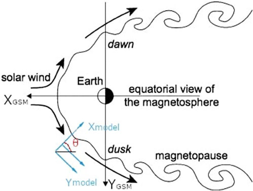
Figure 1. Schematic representation of the low-latitude boundary layer in the Earth’s equatorial plane. Adapted from: Sibeck et al. (2011).

The governing MHD equations are derived for an incompressible, viscous, electrically-conductive fluid with the following simplification: the derivatives of all the parameters along the z-direction are assumed to be zero. The dimensionless form of the MHD equations is provided in the Supplementary Materials of the paper.

For reader reference here we report the GSM reference with respect to the chosen model reference frame. In fact, the computational reference frame varies w.r.t. the GSM magnetopause reference frame depending on the position of the spacecraft along the magnetopause. More in detail, the x-axis is normal to the magnetopause layer and points towards the magnetosphere, the y-axis and z-axis are on the tangent plane to the magnetopause (see Figure 1). We assume that the front side of magnetopause can be approximated as an elliptical paraboloid. If we intersect this figure with the XY and XZ planes of the GSM system, we obtain two parabolas on the same partition planes, each having an equation of the form:

$\chi =a{\gamma }^2+b\gamma +cwitha<0.(1)$

Following this scheme, the position of the spacecraft allows to derive the shape of each parabola. To make the desired change of coordinates it is necessary to calculate the “longitude” θ, defined as the angle between the x-axis of the model and the one of the GSM system on the plane x-y, and the “latitude” α, defined in the same way but on the plane x-z.

To calculate the coefficients of Eq. (1), first we assume that the Earth is located at the parabola’s focus

$F=\left(\frac{1-\mathrm{\Delta }}{4a},-\frac{b}{2a}\right)=\left(\mathrm{0,0}\right).(2)$

so that we can rewrite the Eq. 2 as

$\chi =a{\gamma }^2+\frac{1}{4a}witha<0.(3)$

First, we solve Eq. (3) using the spacecraft’s position to find the coefficient a. After that we calculate the tangent of the parabola at the point where the spacecraft is located, i.e., the derivative of the equation of the parabola. Last, we derive the angles as follows:

$\theta =-arctg\left(\frac{d\chi }{d\gamma }\right)\alpha =-arctg\left(\frac{d\chi }{d\gamma }\right).(4)$

Using Eq. 4 we obtain the following rotation matrices:

$R\left(\theta \right)=\left[\begin{array}{ccc}\hfill \cos \left(\theta \right)\hfill & \hfill -\sin \left(\theta \right)\hfill & \hfill 0\hfill \\ \hfill \sin \left(\theta \right)\hfill & \hfill \cos \left(\theta \right)\hfill & \hfill 0\hfill \\ \hfill 0\hfill & \hfill 0\hfill & \hfill 1\hfill \end{array}\right](5)$

and

$R\left(\alpha \right)=\left[\begin{array}{ccc}\hfill \cos \left(\alpha \right)\hfill & \hfill 0\hfill & \hfill \sin \left(\alpha \right)\hfill \\ \hfill 0\hfill & \hfill 1\hfill & \hfill 0\hfill \\ \hfill -\sin \left(\alpha \right)\hfill & \hfill 0\hfill & \hfill \cos \left(\alpha \right)\hfill \end{array}\right](6)$

Doing the matrix product

$T=R\left(\alpha \right)\cdot R\left(\theta \right)\cdot T_{\text{GSM}}(7)$

where

$T_{\text{GSM}}=\left[\begin{array}{c}\hfill -x\hfill \\ \hfill y\hfill \\ \hfill z\hfill \end{array}\right]andT=\left[\begin{array}{c}\hfill x\hfill \\ \hfill y\hfill \\ \hfill z\hfill \end{array}\right](8)$

we are able to calculate the final parameters’ components in the new spacecraft system.

For example, B_x, B_y and B_z components in our computational reference frame correspond to -$B_x^{\text{GSM}}$, $B_y^{\text{GSM}}$ and $B_z^{\text{GSM}}$ components of the magnetic field at the subsolar point, respectively. Supplementary Table S3 summarises the correspondence between the GSM coordinate system and the computational coordinate system.

The used approach is flexible enough to represent any position on the dayside magnetopause by posing appropriate boundary conditions (see Supplementary Materials), provided the magnetosheath solution is available. The length scale of the imposed perturbation, L, is calculated as the distance covered by the spacecraft to cross the magnetopause.

4 Kelvin-Helmholtz and tearing-mode instabilities

In this section we investigate the presence of KH and TM instabilities, within the Earth’s magnetopause, in response to 21 June 2015 and 6 September 2017 events. Then, using the data provided by different spacecraft we simulate the development and evolution of the instability with our MHD model. This study has been performed following several necessary steps, as follows: (i) inspect the position of spacecraft, (ii) analyse the plasma and magnetic field data to describe the response to the shock impact, (iii) derive the spatial and temporal properties of the magnetopause crossing by the spacecraft, (iv) analyse the plasma and magnetic field parameters during this passage, to identify signatures of KHWs, (iv) extract the proton density, velocity and magnetic field components at the innermost and outermost region of the magnetopause and using them as input parameters for (v) running MHD instability simulations.

4.1 Event 1: 22–23 June 2015

4.1.1 The spacecraft position and the shock-3 arrival

Figure 2 shows the spacecraft orbits at the shock-3 impact, i.e., at 18:34 UT on 22 June 2015. As one can see, THEMIS and Cluster constellations were located at the magnetosheath and no magnetopause crossing were observed. However, the collected data provided key information on the processes produced by the magnetic cloud arrival. Due to their tetrahedral configuration, the four Cluster spacecraft–as well as the three THEMIS spacecrafts - are unique laboratories for investigating the spatial properties of KHWs, because it allows multipoint in situ measurements.

Figure 2

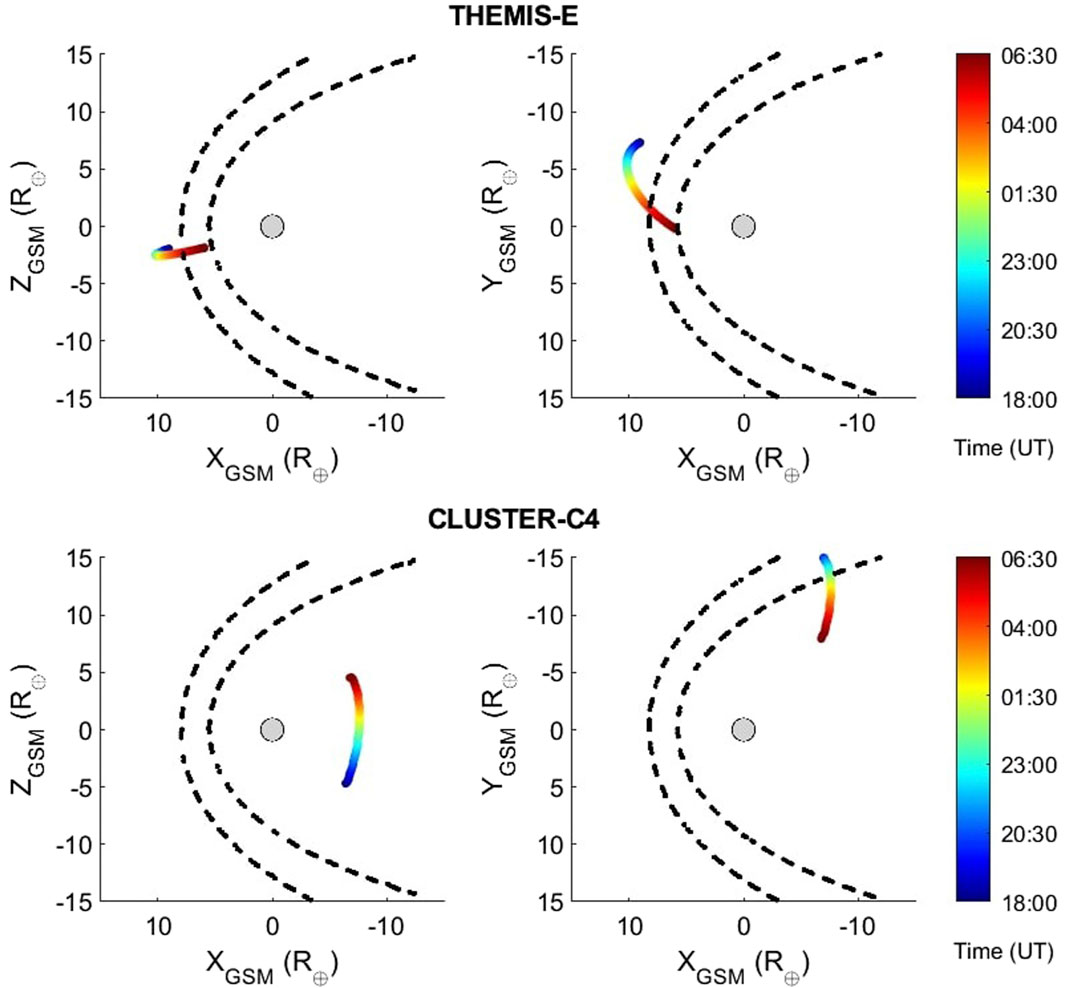
Figure 2. Spacecraft position between 18:00 UT on 22 June 2015 and 06:30 UT on 23 June 2015. Coordinates are expressed in GSM system. Left panel: X-Z plane. Right panel: X-Y plane. Dashed lines indicate the Shue et al. (1998) magnetopause model, at 18:00 UT and 06:00 UT.

During this period the spacecraft THEMIS-E was at the equatorial nose (X_GSM = 9.2, Y_GSM = −7.1, Z_GSM = −2.5 R_⊕), whereas Cluster-C4 was at the equatorial dawnward flank (X_GSM = −6.4, Y_GSM = −15.0, Z_GSM = −5.3 R_⊕). Therefore these two spacecraft offer an excellent opportunity to investigate Case-1 event at two very important magnetopause locations for the transfer plasma momentum in Earth’s magnetosphere.

The IP shock-3 was firstly detected by the ACE spacecraft at L1 (see Supplementary Figure S5). As previously noted in Section 2, ACE recorded an enhancement both in density (Δρ ∼25 p cm⁻³) and in radial velocity (Δv ∼200 km s⁻¹). After ∼30 min, the shock-3 was detected by the Cluster-C4 (see Supplementary Figure S13, left) and THEMIS-E (see SSupplementary Figure S13, right) spacecraft. Data from ACE, Cluster-C4, and THEMIS-C show that the enhancement in the plasma parameters was kept during the propagation towards Earth. The shock-3 produced a variation in solar wind velocity, in IMF strength and in IMF z-component (see Supplementary Table S4). More precisely, Cluster-C4 revealed two small and rapid enhancements of B_z (ΔB_z ∼ 37 nT) due to the magnetic field compression shortly before the transition from about 25 nT to −60 nT. Suvorova et al. (2005) and Piersanti et al. (2017) suggested that these signatures could be a result of the magnetopause crossing.

As a consequence of the shock arrival the magnetopause moved inward reaching a minimum distance of about 5 R_⊕ at 20:00 UT and stabilised at about 8 R_⊕ till 03:00 UT on June 23. Supplementary Figure S14 reports the standoff distance of the magnetopause at the local noon from June 21 to June 24, calculated by empirical models (Space Weather Modeling Framework (SWMF) coupled with the Rice Convection Model (RCM)) using real-time solar-wind data.

4.1.2 Cluster-C4: solar wind and magnetic field parameters

Figure 2 shows the position of Cluster-C4 between June 22 at 18:00 UT and June 23 at 04:00 UT. Due to its polar orbit the spacecraft was travelling along the dawnside flank, mainly in the X-Z plane, close to the equatorial plane. The spacecraft was situated between −7.2 R_⊕ (at 00:00 UT) and −7.3 R_⊕ (at 02:00 UT) along the GSM x-axis, −13.4 R_⊕ and −12.4 R_⊕ along the GSM y-axis and −2.4 R_⊕ and −0.1 R_⊕ along the GSM z-axis. Figure 3 presents an overview of plasma and magnetic field parameters detected by the Cluster-C4 spacecraft¹. The plasma parameters (e.g., proton velocity and density) remained nearly constant in the period June 22 at 23:00 UT and June 23 at 01:00 UT. Similarly, the x- and y-components of the magnetic field (3a-3b) were very steady in the same period, whereas the z-component (3c) was northward. The latter is a key condition for the development of KH waves, as shown in Fairfield et al. (2000) and Ivchenko et al. (2000). Figure 3D reports the strength of the magnetic field. Plasma density and velocity are shown in panels 3e-3f, respectively. Two distinct patterns can be identified. On one hand, the plasma density slightly decreases from ρ = 10 p cm⁻³ (23:00 UT) to ρ = 4 p cm⁻³ (02:30 UT) and it remains constant at about 0.5 p cm⁻³. On the other hand, the plasma velocity lasted nearly constant, v ∼ 400 km s⁻¹, till 01:00 UT and then oscillated around 100 km s⁻¹. Panels 3g-3i show the proton and electron energy spectrogram and the electron pitch angle distribution between 500 and 1,500 eV. As it can be seen, fluctuations in these parameters became clearly visible around 00:00 UT, suggesting that the spacecraft may have encountered multiple magnetopause crossings.

Figure 3

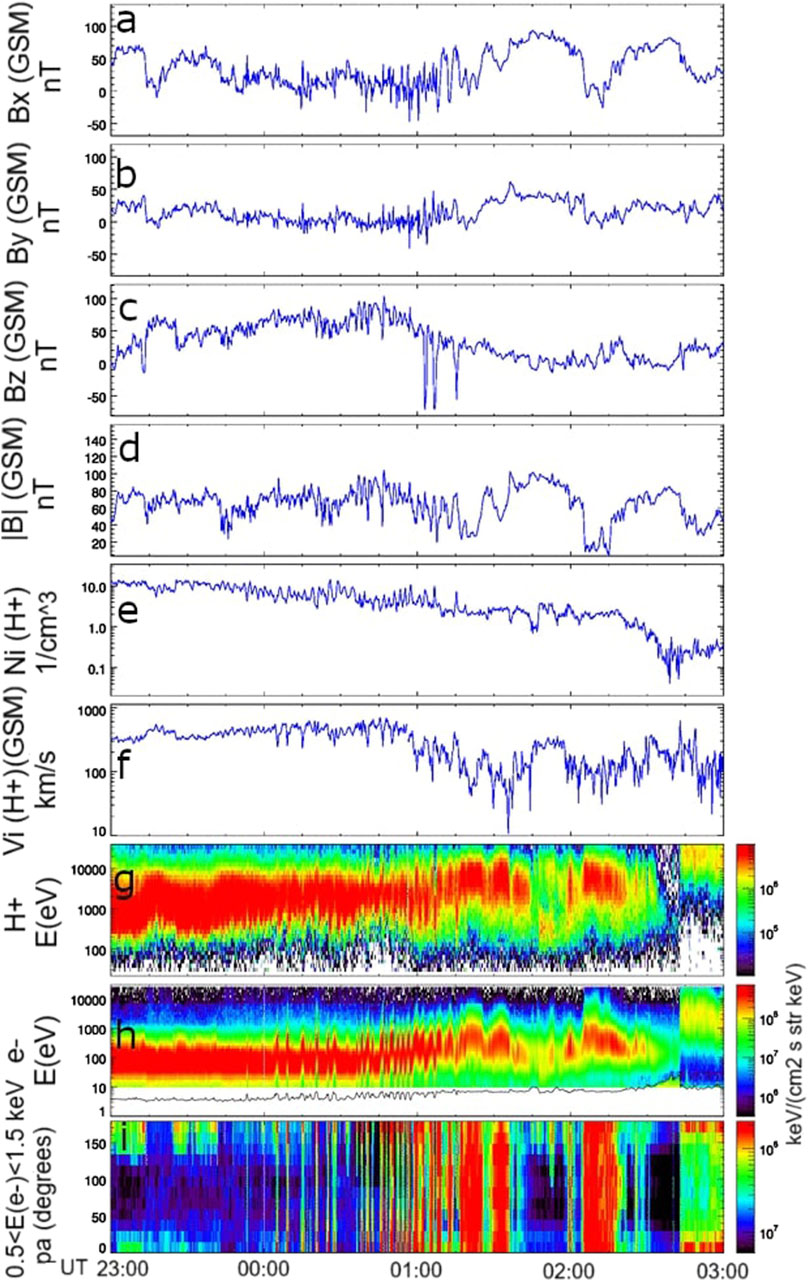
Figure 3. Proton plasma and magnetic field measurements made by Cluster between 22 June 2015 at 23:00 UT and 23 June 2015 at 03:00 UT. Panel (A–C): field components. Panel (D): total field. Panel (E): proton density. Panel (F): proton speed. Panel (G–H): proton and electron energy spectrogram. Panel (I): electron pitch angle distribution between 500 and 1,500 eV. Credits: ESA/Cluster.

Supplementary Figure S15 shows the Cluster-C4 data from 00:40 to 01:00 UT. Several current sheet crossings are visible in the magnetic field measurements, as an abrupt transition of B_y component (panel b). According to Vernisse et al. (2016) these signatures might indicate the crossing of the trailing edge of a KH wave (e.g., Figure 6 in Hasegawa et al., 2009). This hypothesis is supported by another observational signature, i.e., the density reversal (panel e), that characterises rolled-up vortices. This signature is produced by layers of high density that are interposed by layers of lower density. The reader must note that the density reversal appeared soon after the B_y reversal (solid vertical pink lines). However, it is worth mentioning that sawtooth signatures are not visible in the magnetic field, questioning the presence of nonlinear KHWs. In fact, the presence of sawtooth-like structures and their quasi-periodicity are the main of three criteria used to identify nonlinear KHWs (see Section 1). Lastly, it is crucial to emphasize that any observed KH waves are unlikely to be locally produced by the KH mechanism but, rather, indicate a global-scale phenomenon.

Between 02:05 and 02:20 UT the spacecraft crossed an isolated blob of plasma, characterized by reduced |B| and enhanced flux of low-energy ions and electrons ($<$ 2 keV). The latter may have been produced as a result of the detachment of vortices, which could be a post-development of KHIs. Cluster-C4 entered the magnetosphere at about 02:45 UT.

4.1.3 THEMIS-E: solar wind and magnetic field parameters

An analogous analysis has been performed for the THEMIS data. Figure 2 shows the location of THEMIS-E from 18:00 UT on June 22 to 06:30 UT on June 23. During this period the spacecraft was moving earthward along the nose, in proximity to the equatorial plane. Figure 4 presents the plasma and IMF parameters. Note that plasma and magnetic field parameters remained nearly constant until June 23 at 04:37 UT, i.e., the entry within the magnetopause. During this transition the magnetic field components changed: specifically B_x increased from about −20–30 nT, B_y decreased from ∼ 40 nT to ∼ 0 nT and B_z increased of about −80–90 nT (Figure 4B). Similarly, plasma parameters experienced several fluctuations: the proton density reduced of nearly 10 p cm⁻³ (Figure 4C), the electron density reduced of 10 p cm⁻³ (Figure 4D), reduced proton pressure of nearly 1,000 eV cm⁻³ (Figure 4E), the anti-sunward flow velocity reduced of about 50 km s⁻¹ (Figure 4F) and enhanced ion and electron flux of energy $>$1 keV (Figures 4G,H). Upon closer examination of the data, it is observed that a train of low-amplitude fluctuations persisted for up to 1 h (05:45 UT). These structures can be explained either with ion plasma transport within the magnetosphere due to the onset of the magnetic reconnection or by the magnetopause compression caused by the impact of shock-3. In case of magnetic reconnection at the nose, the KH and TM instability could develop and be responsible for propagation of the magnetospheric feature originated after the shock-3 arrival. In the next subsection we study the plausibility of this scenario. Alternatively, in case of magnetosphere compression, the original shock propagates within the magnetosphere, and then it is followed by a reverse-going wave reflected from the denser regions closed to the Earth (e.g., Andréeová and Přech, 2007). Such compression scenario aligns with the observations made by THEMIS-E that registered the vanishing of the event at about 06:00 UT. During this period the spacecraft was situated between 7.3 (at 04:45 UT) and 6.0 (at 05:45 UT) R_⊕ along the GSM x-axis, −0.7 and 0.2 R_⊕ along the GSM y-axis and −2.1 and −1.9 R_⊕ along the GSM z-axis.

Figure 4

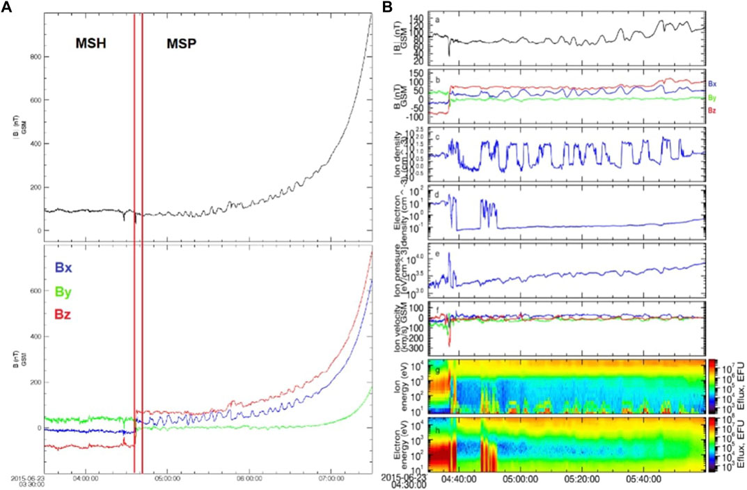
Figure 4. (A): Magnetic field strength and components provided by THEMIS-E spacecraft during 03:30–07:30 UT on 23 June 2015. (B): Overview of proton plasma and magnetic field parameters. Panel (a, b): magnetic field strength and components. Panel (c): proton density. Panel (d): electron density. Panel (e): proton pressure. Panel (f). proton velocity components (v_x: blue, v_y: green and v_z: red). Panel (g) proton energy spectrogram. Panel (h): electron energy spectrogram. Credits: THEMIS-E.

Differently to the data reported by Cluster-C4 (Supplementary Figure S15), no current sheet crossings are visible in the magnetic field measurements. A detailed analysis of the magnetosphere low-amplitude oscillations in the magnetic field data shows a two-phase behaviour - a gradual increasing phase followed by an abrupt decreasing phase. On the other hand, in the ion density data, a box-like pattern appeared as a result of the spacecraft’s transition through a mixing region of magnetosheath and magnetospheric plasma.

4.1.4 MHD instability simulations

In this section, a set of MHD simulations for Case-1 are discussed. The flexibility of the model allows for the representation of any position on the dayside equatorial magnetopause by adjusting the appropriate input parameters.

Table 1 provides a summary of the characteristics of the magnetosheath and magnetosphere regions, including the total magnetic field, its components and the proton density.

Table 1

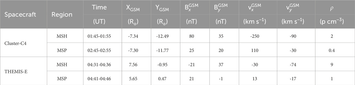
Table 1. Case 1. Magnetic and plasma data at the magnetosheath (MSH) and magnetospheric (MSP) boundaries of the magnetopause.

Regarding the Mach and the Reynolds numbers, specific considerations need to be taken into account.

The Mach number can be derived from the following equation:

$M_A=\frac{v_{SH}}{v_A}=\frac{v_{SH}}{|B|}\sqrt{\rho {\mu }_0{m}_p}(9)$

where v_SH is the sheath flow velocity and v_A is the Alfven velocity. The latter is proportional to the ratio between the total magnetic field (|B|) and the square root of the number ion density, ρ, the mass of the proton, m_p, and the vacuum magnetic permeability, μ₀. Thus, using the THEMIS-E data from the period between 04:31 and 04:36 UT, we choose v_SH = 85 km s⁻¹, |B| = 90 nT and ρ = 9 p cm⁻³, and derive M_A = 0.1. On the other hand, using Cluster-C4 data, we choose v_SH = 250 km s⁻¹, |B| = 95 nT and ρ = 2 p cm⁻³, and derive M_A = 0.2.

The Reynolds number (R_e) and its magnetic counterpart, R_m, are defined as follows:

$R_e=\frac{v_{SH}L}{\nu }(10)$

$R_m=\frac{v_{SH}L}{\eta }(11)$

where L is the characteristic length of the transition layer, ν is the kinematic viscosity and η the magnetic diffusivity. Distinct methods can be adopted to retrieve ν, for example, the gyrotropic motion of solar wind particles (e.g., Pérez-de-Tejada, 1999). In fact, due to the thermal motion produced by the velocity shear, momentum transport and exchange occur. Assuming that the first mechanism occurs via wave-particle interaction, then Ω_p and n_p are the frequency of the interaction and the particle density, respectively. Concerning the exchange by SW protons it occurs via a full period around their Larmor radius, r_L. Then, the kinematic viscosity obtained by Newcomb (1966) is defined as follows:

$\nu =\frac{\mu }{n_p{m}_p}=r_L^2{\mathrm{\Omega }}_p(12)$

where m_p is the mass of protons and μ the viscosity coefficient. Calculations of the transport of momentum to the Earth’s magnetosphere have provided values of kinematic viscosity of about 800 km² s⁻¹ (Eviatar and Wolf, 1968). This value is close to the viscosity previously estimated by Axford (1964), ν = 10³ km² s⁻¹, which satisfies the energy requirements for a typical magnetic storm. Haerendel et al. (1978) suggested that the magnetic diffusivity, η, is of the same order. A subsequent study conducted by Verma (1996) indicated that ν = 200 km² s⁻¹ and η = 50 km² s⁻¹, i.e., a ratio of about 4.

In the case of THEMIS-E, assuming L = 1,000 km (Le and Russell, 1994) as the thickness of the magnetopause at the nose, v_SH = 150 km s⁻¹, ν = 1,000 km² s⁻¹ and η = 250 km² s⁻¹ we obtain R_e = 150 and R_m = 600, respectively. In the case of Cluster-C4, assuming L = 1,000 km, v_SH = 250 km s⁻¹, ν = 1,000 km² s⁻¹ and η = 250 km² s⁻¹ we obtain R_e = 250 and R_m = 1,000, respectively.

In the following, we describe the results of the MHD simulations firstly adopting the THEMIS-E data and, then, adopting the Cluster-C4 data.

In the case of the THEMIS-E data, the results for the time evolution of dimensionless density and B_y are shown in Figures 5, 6, respectively. It is important to point that at the magnetopause nose no rolled-up KHVs can develop due to the absence of a shear between the two fluids (Foullon et al., 2008; Farrugia and Gratton, 2011) and sufficient time, i.e., the MR can occur only through the tearing mode instability. In this sense, the MHD simulation confirms that no KHVs developed at the nose. Note that disturbances formed very fast, since they are noticeable after 1 s of computational time (t_comp) (defined as $t_{\mathit{comp}}=\frac{L}{v_{SH}}t$), where one second of computational time corresponds to ∼ 0.15 s. Furthermore, the amplitude of the disturbance narrowed with time, vanishing at 8 computational seconds. Concerning the TM instability, Figure 6 shows that structures similar to magnetic islands appeared in B_y component very fast, at 1 computational second. However, the system experienced a rapid suppression, i.e., magnetic islands vanished for 10 computational seconds. These structures are characterised by discrete parallel filaments (formed by the phenomenon known as sheet pinch) that have the potential to tear along the lines of current flow (Furth et al., 1963). Magnetic islands at the magnetopause can facilitate the entry of plasma and energy within the magnetosphere. Therefore, their presence is important because it could explain the formation of the train of low-amplitude fluctuations, who persisted from 04:40 UT to 05:45 UT.

Figure 5

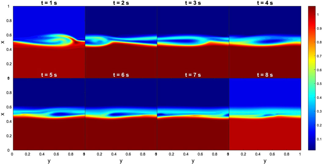
Figure 5. Case 1. Evolution of KH instabilities in density at the nose of the magnetopause, from 1 to 8 s. Input data obtained from the THEMIS-E measurements. The dimensionless boundary conditions from the magnetosphere side and magnetosheath side are taken everywhere to be identical: $B_x^{\mathit{MSP}}$ = -0.9, $B_x^{\mathit{MSH}}$ = 1.0, $B_y^{\mathit{MSP}}$ = 0.0, $B_y^{\mathit{MSH}}$ = 1.0, ρ^MSP = 0.1, ρ^MSH = 1.0. R_e = 84 and R_m = 337. M_A = 0.1. Blue region represents the magnetosphere whilst red region represents the magnetosheath.

Figure 6

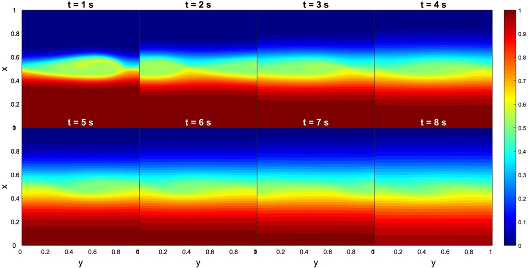
Figure 6. Case 1. Evolution of TM instabilities in B_y at the nose of the magnetopause, from 1 to 8 s. Input data obtained from the THEMIS-E measurements. The dimensionless boundary conditions from the magnetosphere side and magnetosheath side are taken everywhere to be identical: $B_x^{\mathit{MSP}}$ = -0.9, $B_x^{\mathit{MSH}}$ = 1.0, $B_y^{\mathit{MSP}}$ = 0.0, $B_y^{\mathit{MSH}}$ = 1.0, ρ^MSP = 0.1, ρ^MSH = 1.0. R_e = 84 and R_m = 337. M_A = 0.1. Red region represents the magnetosphere whilst blue region represents the magnetosheath.

In the case of the Cluster-C4 data, Figure 7 shows the onset of KHIs at the dawnward flank of the magnetopause. More specifically, KHVs develop within only 2 computational seconds and persists up to 20 computational seconds, manifesting almost steady state of the MHD instability. Concerning the time evolution of dimensionless B_y, we find the early development of the TM instability (see Figure 8), i.e., magnetic islands appeared at the first computational second. Contrary to KHI, for 10 computational seconds these structures had already vanished. Note, that the analysis of Cluster data reports high flow shear between the two regions (Δv ∼ 300 km s⁻¹) together with low magnetic shear (Δ|B|∼ 20 nT). These observations are in agreement with the theoretical predictions, confirming that regions with high flow shear and low magnetic shear triggers KHIs (Foullon et al., 2008). Correspondingly, the TM instability is damped for the half of the time needed for the development of the KHI. In global scale, these findings indicate that wave perturbations become unstable far away from the subsolar point in the direction of high flow shear.

Figure 7

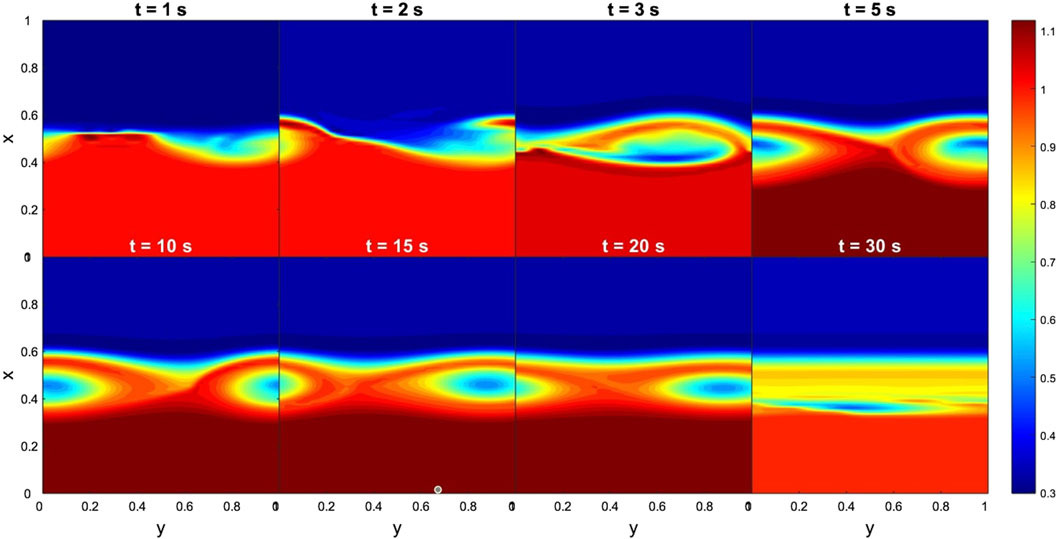
Figure 7. Case 1. Evolution of KH instabilities in density at the dawnward flank of the magnetopause, from 1 to 30 s. Input data obtained from the Cluster-C4 measurements. The dimensionless boundary conditions from the magnetosphere side and magnetosheath side are taken everywhere to be identical: $B_x^{\mathit{MSP}}$ = -1.24, $B_x^{\mathit{MSH}}$ = 1.0, $B_y^{\mathit{MSP}}$ = 0.4, $B_y^{\mathit{MSH}}$ = 1, ρ^MSP = 0.2, ρ^MSH = 1, R_e = 250 and R_m = 1,000, M_A = 0.2. Blue region represents the magnetosphere whilst red region represents the magnetosheath.

Figure 8

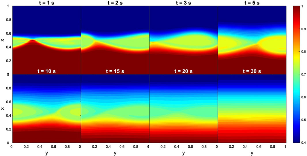
Figure 8. Case 1. Evolution of TM instabilities in B_y at the dawnward flank of the magnetopause, from 1 to 30 s. Input data obtained from the Cluster-C4 measurements. The dimensionless boundary conditions from the magnetosphere side and magnetosheath side are taken everywhere to be identical: $B_x^{\mathit{MSP}}$ = -1.24, $B_x^{\mathit{MSH}}$ = 1.0, $B_y^{\mathit{MSP}}$ = 0.4, $B_y^{\mathit{MSH}}$ = 1, ρ^MSP = 0.2, ρ^MSH = 1, R_e = 250 and R_m = 1,000, M_A = 0.2. Blue region represents the magnetosphere whilst red region represents the magnetosheath.

4.1.5 The reconnection rate

The reconnection rate, which represents the speed at which magnetic field lines are rearranged and energy is released, can be influenced by the presence of KH and TM instabilities. Dimensionless reconnection rate α (Sonnerup et al., 1981; Mozer and Retinò, 2007; Mozer and Hull, 2010) is defined as:

$\alpha =\frac{B_N}{B_{MP}}=\frac{V_{IN}}{V_A}.(13)$

where B_N represents the normal component of the magnetic field respect to the magnetopause and is averaged across the magnetopause. The magnitude of the magnetic field, B_MP, is derived immediately inside the magnetopause current layer (Jia et al., 2019). Similarly, the reconnection rate can be derived as the ratio between the plasma inflow speed (V_IN) and the outflow jet velocity (V_A) of the open flux tubes. The THEMIS-E and MF data confirm a reconnection rate α = 0.05 (Eq. 13), i.e., nearly identical with respect to the best available statistical value of 0.046 at Earth (Mozer and Retinò, 2007). The MHD simulation reveals an increase of the reconnection rate after about 8 computational seconds after the entry in the magnetopause equal to 0.30. Unfortunately due to the geometrical configuration of the Cluster-C4 observations it is difficult to identify the exact passage through the magnetopause and hence to calculate the reconnection rate. According to Dibraccio et al. (2013), since α is dimensionless the dependence of flux transfer rate on the strength of the magnetic field is removed.

4.2 Event 2: 7–8 September 2017

4.2.1 The spacecraft position and the shock-2 arrival

Figure 9 shows the spacecraft orbits during the shock impact, that occurred at about 23:00 UT on 7 September 2017. Notably, three distinct spacecraft constellations crossed the magnetopause during the subsequent 12 hours: THEMIS, Cluster and MMS. Among them, THEMIS and Cluster were both located at the nose of the magnetopause but at different altitude: THEMIS-E at the equatorial nose (X_GSM = 11.4, Y_GSM = 2.1, Z_GSM = −0.7 R_⊕), whereas Cluster-C4 at the middle-altitude nose (X_GSM = 4.2, Y_GSM = 2.8, Z_GSM = 5.0 R_⊕). This spatial configuration represents a valuable test for investigating the response of the magnetopause to the dynamic pressure exerted by the shock-2. At the same time, MMS1 was located closer to the Earth (X_GSM = 1.8, Y_GSM = 1.3, Z_GSM = −0.6 R_⊕).

Figure 9

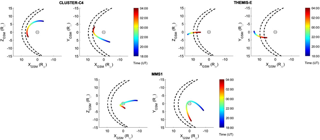
Figure 9. Location of the Cluster-C4, THEMIS-E and MMS1 spacecraft between 18:00 UT on 7 September 2017 and 04:00 UT on 8 September 2017. Note that the shock arrived at ∼ 23:00 UT on September 7. Coordinates are expressed in GSM system. Each panel shows both the X-Y and the X-Z plane. Dashed lines indicate the compression of the magnetopause computed with the Shue et al. (1998) magnetopause model.

Figure 10

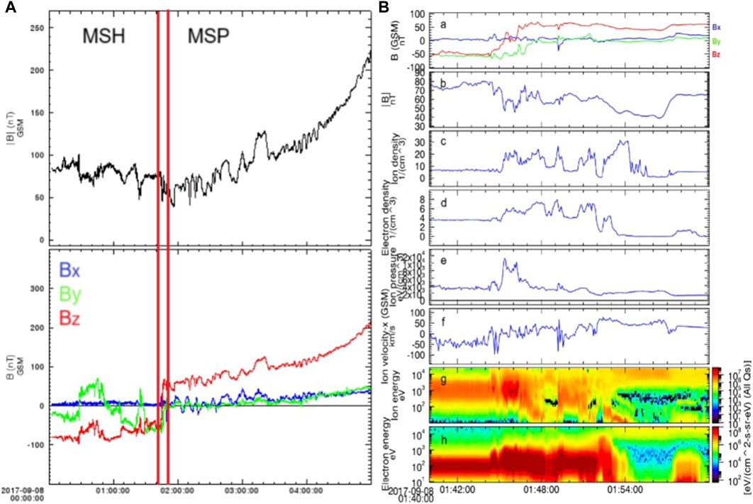
Figure 10. (A): Magnetic field strength and components provided by THEMIS-E spacecraft during 00:00–05:00 UT on 8 September 2017. (B): Overview of proton plasma and magnetic field parameters. Panel (a) magnetic field components (Bx: blue line, By: green line and Bz: red line). Panel (b) magnetic field strength. Panel (c) proton density. Panel (d) electron density. Panel (e) proton pressure. Panel (f) x-component of proton velocity. Panel (G) proton energy spectrogram. Panel (h) electron energy spectrogram. Credits: THEMIS.

Figure 11

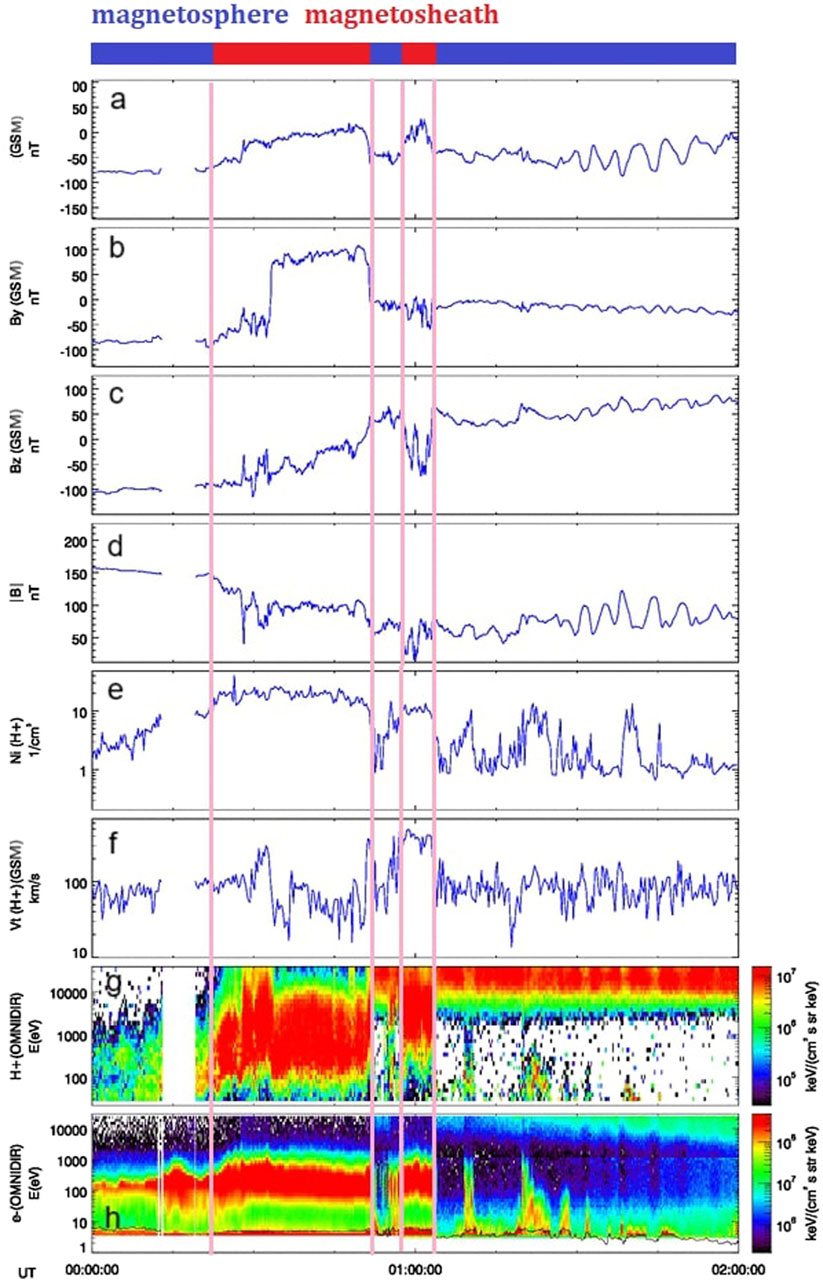
Figure 11. Overview of proton plasma and magnetic field measurements made by Cluster-C4 between 00:00–02:00 on 8 September 2017. Panel (A–C): Magnetic field components. Panel (D): Total field. Panel (E): proton density. Panel (F): proton velocity. Panel (G, H): proton and electron energy spectrogram. Credits: ESA/Cluster.

The shock-2 produced by the CME-3 event was firstly detected by the ACE satellite, at 22:34 UT on 7 September 2017. We reported in Supplementary Figure S11 the relative enhancement in SW density, radial velocity and temperature and in the IMF. After nearly 26 min (at ∼ 23:00 UT), the shock-2 was detected by THEMIS-E and by Cluster-C4 spacecraft (see Supplementary Figure S16). We summarise in Supplementary Table S5 the variation in the plasma and IMF data induced by the shock-2. Unfortunately, no data were reported by MMS spacecraft due to its very close position to Earth (∼2 R_⊕).

As a result of the interaction between the ICME and the planet’s magnetosphere significant perturbations in the position of the bow shock and the magnetopause were caused. In fact, due to the increased dynamic pressure exerted by the interplanetary shock-2, the bow shock region moved earthward as well as the magnetopause compressed (the subsolar point was moved to $\sim 6R_{\oplus }$ at about 00:00 UT, see Supplementary Figure S17).

4.2.2 Plasma and magnetic field parameters

In this section, we present an overview of the data measured by the three spacecraft. Unfortunately the particle data from the fast plasma investigation instrument (Pollock et al., 2016), on board MMS, were not retrieved:

• Figure 9 shows that, due to its position, THEMIS-E remained within the magnetosheath region during the period 20:00–02:00 UT. With the arrival of the shock-2, the spacecraft experienced a series of oscillations in the magnetic field components (right panel of Supplementary Figure S4A–D) and strength (right panel of Supplementary Figure S4D) as well as in plasma density (right panel of Supplementary Figure S4E) and velocity (right panel of Supplementary Figure S4F). Notably, B_x and B_y reversed, B_z decreased from about −34 to −73 nT and |B| increased from ∼ 43 to ∼ 83 nT (see Supplementary Figure S5). Only at the end of the event, when the dynamic pressure exerted by the ICME weakened and the magnetopause returned to its original location (∼10 R_⊕), THEMIS-E crossed the nose of the magnetopause, at about 02:00 UT on September 8. Importantly, this interaction lasted only a few minutes as the spacecraft was moving earthward whilst the magnetopause sunward. This scenario has been confirmed by the analysis in the period 01:40–02:00 UT (see Figure 10). The spacecraft moved from a more-magnetosheath region (at 01:40 UT) to a more-magnetospheric region (at 01:55 UT) in nearly 10 min. During this transition B_z and B_y gradually reversed from −50 to 50 nT and from −55 to 10 nT (Figure 10A), respectively. At the same period, |B| decreased (Figure 10B) whereas plasma parameters (e.g., ion/electron density, Figures 10C, D) experienced several oscillations.

• Figure 9 illustrates the orbit of Cluster-C4 between 18:00 UT on September 7 and 04:00 UT on September 8. The arrival of the shock-2 at 23:00 UT was documented by the variation in the plasma and IMF parameters (see Supplementary Figure S5). Cluster-C4 crossed the magnetopause at about 01:00 UT (lower right panel). Figure 11 illustrates the plasma and IMF parameters during the period 00:00–02:00 UT on September 8. Vertical solid pink lines delineate different MP crossings, such as the sharp rotation in B components that corresponds to variation in the ion density and velocity. We refer to Section 4.1 for a description of the characteristics that distinguish a more-magnetospheric to a more-magnetosheath region. No KHWs signatures were revealed most probably due to the very low shear that prevented the necessary diffusion rate between the two regions.

     However, starting from about 01:30 UT, another type of dynamic feature can be distinguished near the magnetopause, a flux transfer event (FTE, Russell and Elphic, 1978). FTEs are characterised by bipolar pulse signatures in the IMF normal (in our case B_x) to the unperturbed magnetopause surface (Keith and Heikkila, 2021). They are the results of the passage of flux tubes embedded in the magnetopause with approximate size ∼ 1 R_⊕ and their impulsive reconnection. Typical signatures are visible both in the IMF and SW parameters. On one hand, the IMF exhibits a sharp and rapid rotation as the FTEs cross, indicating magnetic field lines transfer. On the other hand, FTEs are often accompanied by plasma flows across the magnetopause, that can be observed as abrupt changes in the velocity and acceleration into the direction of the plasma particles stream.

4.3 MHD instability simulations

In this section we discuss a set of MHD simulations we performed for Case-2.

We summarise in Table 2 the characteristics of the magnetosheath and magnetosphere regions, including the magnetic field components, the proton velocity components and the proton density.

Table 2

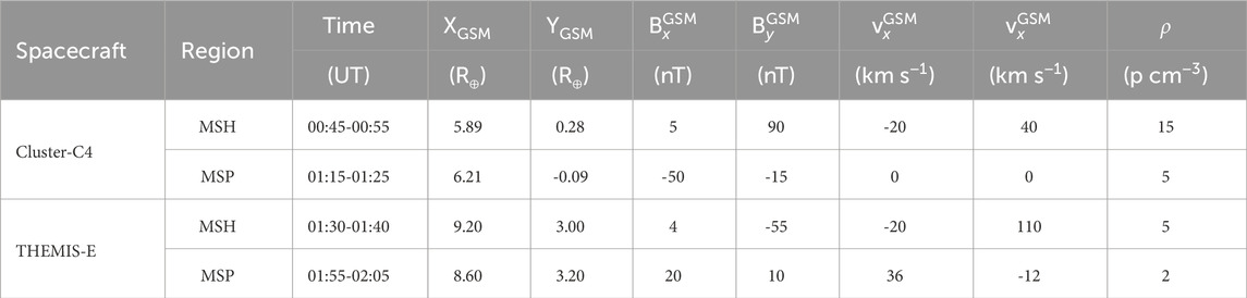
Table 2. Case 2. Summary of the magnetic and plasma data at magnetospheric (MSP) and magnetosheath (MSH) boundaries.

Concerning the Mach and the Reynolds numbers, distinct considerations must be taken into account for the two spacecraft:

• in the case of THEMIS-E, choosing v_SH = 150 km s⁻¹, |B| = 75 nT and ρ = 5 p cm⁻³, and derive M_A = 0.2. Whilst assuming L = 1,000 km, v_SH = 150 km s⁻¹, ν = 1,000 km² s⁻¹ and η = 250 km² s⁻¹ we obtain R_e = 150 and R_m = 600, respectively;

• in the case of Cluster-C4, choosing v_SH = 70 km s⁻¹, |B| = 100 nT and ρ = 15 p cm⁻³, and derive M_A = 0.1. Whilst assuming L = 1,000 km, v_SH = 70 km s⁻¹, ν = 1,000 km² s⁻¹ and η = 250 km² s⁻¹ we obtain R_e = 70 and R_m = 280, respectively.

Here, we describe the results of the MHD simulations firstly adopting the THEMIS-E data and, then, adopting the Cluster-C4 data.

In the case of the THEMIS-E data, the results for the time evolution of dimensionless density and B_y are shown in Figures 12, 13, respectively. As pointed in the previous Section 4.2, owing to its position at the magnetopause nose the MR can occur only through the tearing mode instability. However, in this case no signatures are visible in both Figures 12, 13, indicating that the instability had not developed. These results are expected due to the extremely low flow (Δv ∼ 100 km s⁻¹) and high magnetic shear in each direction (ΔB = 10 nT).

Figure 12

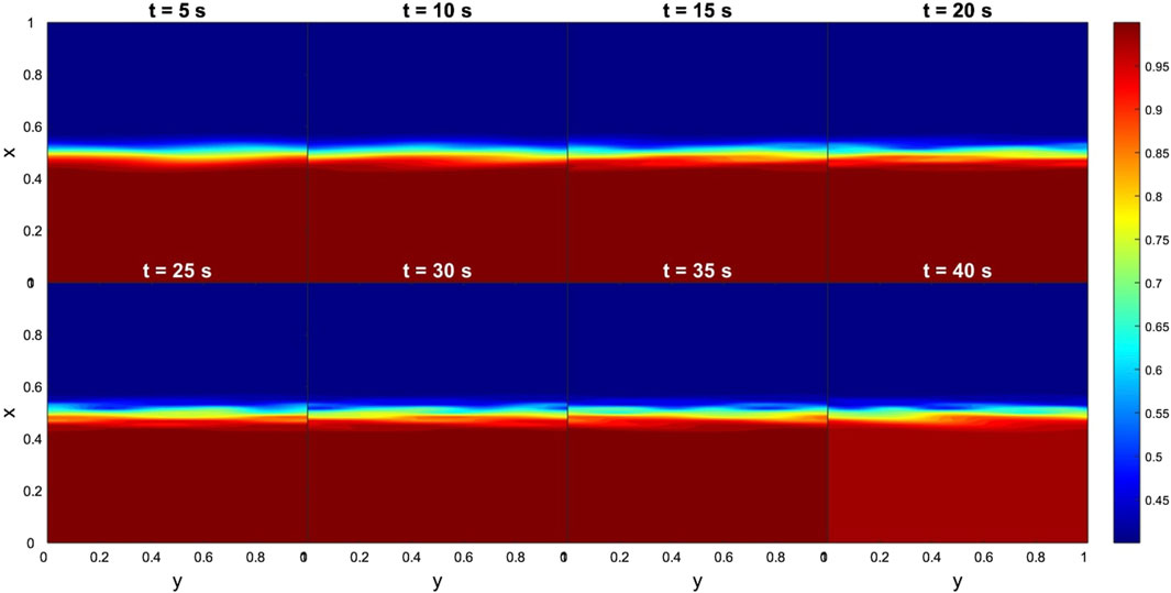
Figure 12. Case 2. Evolution of KH instabilities in density at the nose of the magnetopause, from 5 to 40 s. Input data obtained from the THEMIS-E measurements. The dimensionless boundary conditions from the magnetosphere side and magnetosheath side are taken everywhere to be identical: $B_x^{\mathit{MSP}}$ = 3.0, $B_x^{\mathit{MSH}}$ = 1.0, $B_y^{\mathit{MSP}}$ = -0.27, $B_y^{\mathit{MSH}}$ = 1.0, ρ^MSP = 0.4, ρ^MSH = 1.0. R_e = 150 and R_m = 600. M_A = 0.2. Blue region represents the magnetosphere whilst red region represents the magnetosheath.

Figure 13

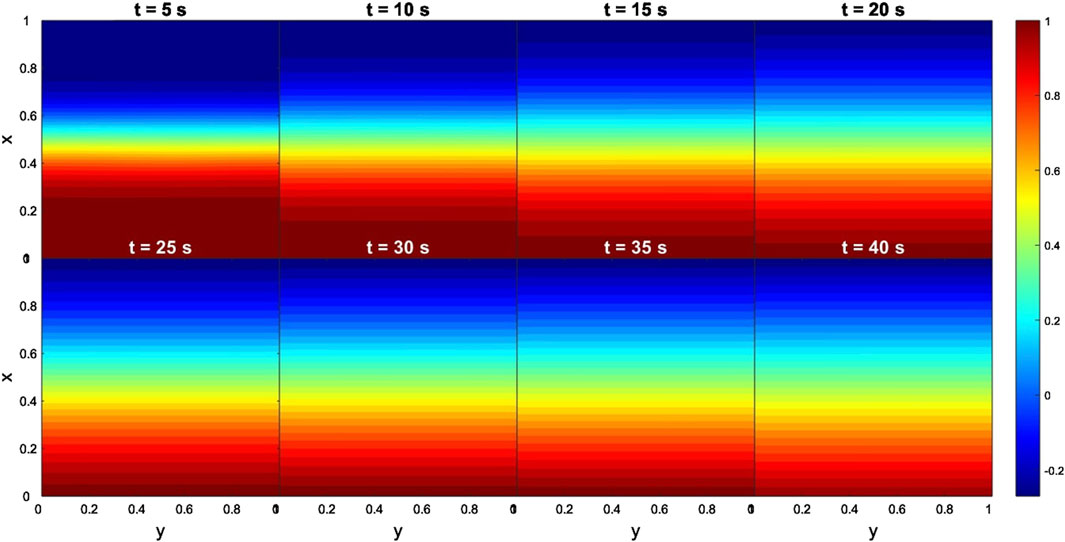
Figure 13. Case 2. Evolution of TM instabilities in B_y at the nose of the magnetopause, from 5 to 40 s. Input data obtained from the THEMIS-E measurements. The dimensionless boundary conditions from the magnetosphere side and magnetosheath side are taken everywhere to be identical: $B_x^{\mathit{MSP}}$ = 3.0, $B_x^{\mathit{MSH}}$ = 1.0, $B_y^{\mathit{MSP}}$ = -0.27, $B_y^{\mathit{MSH}}$ = 1.0, ρ^MSP = 0.4, ρ^MSH = 1.0. R_e = 150 and R_m = 600. M_A = 0.2. Blue region represent the magnetosphere whilst red region represent the magnetosheath.

In the case of the Cluster-C4 data, the results for the time evolution of dimensionless density and B_y are shown in Figures 14, 15, respectively. Figure 14 shows that the fast development of KHIs enhanced disturbances but no signatures of KHVs are visible. Furthermore, at 15 computational seconds these disturbances had already vanished. A similar pattern can be distinguished in the B_y results. Figure 15 shows that magnetic islands appeared very fast, for 1 computational second. However, the system experienced a rapid suppression, i.e., magnetic islands vanished for 5 computational seconds. Similarly to the THEMIS case, these simulation results are expected. More specifically, the extremely low flow (Δv ∼ 100 km s⁻¹) and high magnetic shear by components (e.g., ΔB_x = 16 nT, ΔB_y = 65 nT and ΔB_z = 110 nT) between the two regions, prevent the onset of KHIs (Foullon et al., 2008; Farrugia and Gratton, 2011). Despite the low total magnetic field variation (Δ|B| = 10 nT) between the two regions we obtained TM instability likely due to the high shear in the components of the magnetic field. In a global scale, these findings indicate that the conditions at the nose of the magnetopause at two distinct moments were not favourable for the non-linear development of the KHWs.

Figure 14

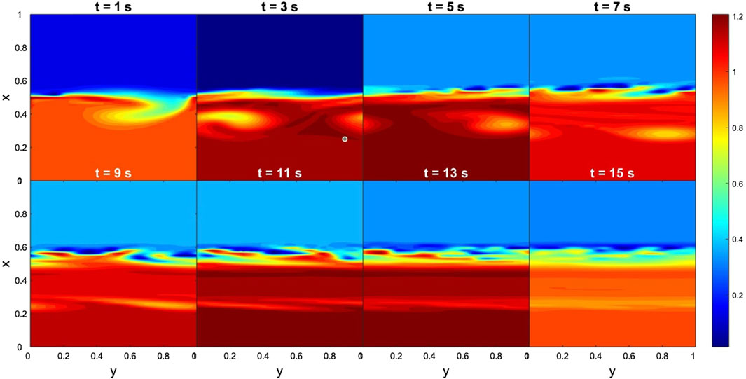
Figure 14. Case 2. Evolution of KH instabilities in density at the nose of the magnetopause, from 1 to 15 s. Input data obtained from the Cluster-c4 measurements. The dimensionless boundary conditions from the magnetosphere side and magnetosheath side are taken everywhere to be identical: $B_x^{\mathit{MSP}}$ = -4.0, $B_x^{\mathit{MSH}}$ = 1.0, $B_y^{\mathit{MSP}}$ = -0.3, $B_y^{\mathit{MSH}}$ = 1.0, ρ^MSP = 0.3, ρ^MSH = 1.0. R_e = 70 and R_m = 280. M_A = 0.1. Blue region represents the magnetosphere whilst red region represents the magnetosheath.

Figure 15

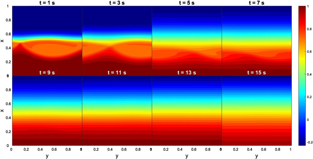
Figure 15. Case 2. Evolution of TM instabilities in B_y at the nose of the magnetopause, from 1 to 15 s. Input data obtained from the Cluster-C4 measurements. The dimensionless boundary conditions from the magnetosphere side and magnetosheath side are taken everywhere to be identical: $B_x^{\mathit{MSP}}$ = -4.0, $B_x^{\mathit{MSH}}$ = 1.0, $B_y^{\mathit{MSP}}$ = -0.3, $B_y^{\mathit{MSH}}$ = 1.0, ρ^MSP = 0.3, ρ^MSH = 1.0. R_e = 70 and R_m = 280. M_A = 0.1. Blue region represents the magnetosphere whilst red region represents the magnetosheath.

4.3.1 The reconnection rate

The Cluster-C4 results confirm a reconnection rate of about α = 0.05. The MHD simulation reveals an increase in the reconnection rate after about 4 computational seconds after the entry in the magnetopause equal to α = 0.50, i.e., nearly ten times higher than the best available statistical value of 0.046 at Earth (Mozer and Retinò, 2007). Concerning the THEMIS-E data, the MHD simulations did not show any magnetic reconnection.

5 Discussions and conclusion

In this work we analysed two distinct events that took place on 22–23 June 2015 (Case-1) and on 6–7 September 2017 (Case-2). Our analysis focuses on the origin of these events on the Sun, their interplanetary propagation and arrival at Earth.

In Case-1, the data collected by Cluster-C4 at the equatorial dawnward flank offer the possibility for a plenty of interpretations. On one hand one of the three observational criteria used to determine the presence of KHI vortices was not satisfied, because the B did not display sawtooth signatures and their quasi-periodicity. On the other hand, several features in the solar wind parameters, such as the crossing of current sheet or the density reversal, could indicate the presence of rolled-up vortices. On the contrary, the box shape pattern in the data measured by THEMIS-E could be interpreted as either the result of shock-induced compression or magnetic reconnection. The latter scenario suggests that the KHIs were present at the equatorial nose and produced a train of waves in the low-amplitude region (04:45–05:45 UT), characterised by a box-like structures in the ion density, that recurred approximately every 5 minutes. We found a reconnection rate α = 0.05 at the magnetopause upon entry and an increased rate of α = 0.30 through a MHD simulation after 4 computational seconds. The increased reconnection rate could be associated with the fact that the normal component of the magnetic field at the entry of the magnetopause is much lower than the one after 1 min, where the spacecraft is close to the magnetosphere. Subsequently, we used our MHD model to interpret observational data and, thus, to investigate the potential development of KHVs on the dawn flank magnetopause as a consequence of the arrival of the flare-associated CME. Using THEMIS-E data, we found that at the magnetopause nose no rolled-up KHVs developed due to the absence of a shear between the two fluids. On the contrary, structures similar to magnetic islands appeared in B_y component very fast (in one computational second) and vanished for 10 computational seconds. At the dawn flank magnetopause, the analysis of Cluster data revealed high flow and low magnetic shear between the magnetosheath and the magnetosphere. According to theoretical predictions, these conditions favour the onset of KHIs instabilities. Indeed, MHD simulations confirmed these considerations, finding that KHVs developed very rapidly and persisted up to 20 computational seconds, reaching almost MHD instability steady state. Regarding the TM instability, the MHD simulations revealed only an early development of magnetic islands, that persisted for half of the time of the KHVs evolution. In a global scale, these results indicate that vortices become unstable far away from the subsolar point in the direction of high flow shear. In Case-1, the development of KHVs may have played a role in enhancing the intensity of geomagnetic storms caused by the shock-3. The dynamic processes initiated by these vortices, even in response to moderate intensity solar events, can support the variation in the geomagnetic indices, for example, K_p= 8+ indicating the intense storm regime followed by a severe storm (K_p = 8-) after 12 hours. In addition, the increase of the plasma reached the magnetosphere is up to 40 p cm⁻³ with the respect to the plasma delivered by quiet solar wind.

In Case-2, the data collected by Cluster-C4 and THEMIS-E at the equatorial nose offered an opportunity to investigate how different regions at the same latitude respond to the dynamic pressure caused by the arrival of the ICME. THEMIS-E provided data from the magnetosheath region, whereas Cluster-C4 from the magnetosphere. Interestingly, similar fluctuations were identified. As a consequence of the arrival of the shock-2 the magnetopause moved earthward, reaching its minimum distance of ∼ 6 R_⊕. At 23:00 UT on 7 September 2017, Cluster-C4 crossed the earthward magnetopause and entered within the magnetosheath. After nearly 2 hours the dynamical pressure reduced and the magnetopause moved back towards the Sun to its original position. Cluster-C4 was the first to encounter the moving magnetopause, at approximately 01:00 UT, followed by THEMIS-E at around 01:40 UT. It must be noted that during these crossings no signatures of KHWs were revealed but clear fluctuations in the magnetic field B_x component indicated the presence of FTEs, which were produced by the passage of flux tubes embedded in the magnetopause. The reconnection rate was found to be α = 0.05, at the magnetopause immediately after its entry and increased up to α = 0.50 after 4 computational seconds as shown in our MHD simulation. Using THEMIS-E data, we did not find any evidence of KH instability owing to the extremely low flow and high magnetic shear. On the contrary, adopting Cluster-C4 data, MHD simulations revealed that the fast development of disturbances (∼ one computational second) but no signatures of KHVs were visible. Additionally, magnetic islands appeared very fast as a result of high shear in the components of the magnetic field but rapidly vanished.

The results reveal that regions of maximum KH growth rates correspond to regions characterized by high flow shear and low magnetic shear. However, in the considered cases, these conditions do not depend on the intensity of the space weather event, defined by the class of the generating flare and the velocity of the associated CME. Our results show the development of KHVs even for a moderate M2.6-class flare with an associated CME shock front with velocity of 750 km s⁻¹. Moreover, we have identified that the minimum shear velocity necessary for the formation of such vortices must be at least 300 km s⁻¹, if low magnetic shear (20 nT) is present. Moreover, these results suggest independence of KHV formation from the extreme nature of space weather events.

Thanks to the KH and TM instability simulations we can estimate the response of the magnetosphere to strong solar eruptions qualitatively through the efficiency of formation of the magnetosphere KH and magnetic island structures as well as reconnection rate variance in the magnetopause. This approach has the potential to be applied to solar flare events that may have a hazard impact on the Earth.

Finally, the current study provides a methodological approach that can be applied also to study other planetary magnetospheres. From a planetary space weather perspective, KH and TM instability simulations can improve significantly our understanding of both the short and long-term of impacts of the Sun-planet interactions (see discussion in Plainaki et al., 2016).

Data availability statement

The original contributions presented in the study are included in the article/Supplementary Material, further inquiries can be directed to the corresponding author.

Author contributions

LB: Conceptualization, Data curation, Formal Analysis, Investigation, Methodology, Software, Writing–original draft. SI: Methodology, Project administration, Software, Supervision, Writing–original draft. LC: Writing–original draft, Data curation. GJ: Writing–original draft. ML: Writing–original draft. DD: Writing–original draft. FL: Writing–original draft. CP: Writing–original draft. MM: Writing–original draft. AM: Writing–original draft. MM: Writing–original draft. CF: Writing–original draft.

Funding

The author(s) declare that financial support was received for the research, authorship, and/or publication of this article. This research was funded by Agenzia Spaziale Italiana and Istituto Nazionale di Astrofisica grant agreement ASI-INAF n.2020-35-HH.0.CAESAR is supported by the Italian Space Agency and the National Institute of Astrophysics through the ASI-INAF n.2020-35-HH.0 agreement for the development of the ASPIS prototype of the scientific data centre for Space Weather. The results have been obtained with the financial support of “Asse IV del PON Ricerca e Innovazione 2014–2020 “Istruzione e ricerca per il recupero–REACT-EU.” We acknowledge support by the INAF with the mini-grant, ‘Space WEather Analysis of Rogue events (SWEAR)’ (F.O. 1.05.23.04.03).

Conflict of interest

The authors declare that the research was conducted in the absence of any commercial or financial relationships that could be construed as a potential conflict of interest.

The author(s) declared that they were an editorial board member of Frontiers, at the time of submission. This had no impact on the peer review process and the final decision.

Publisher’s note

All claims expressed in this article are solely those of the authors and do not necessarily represent those of their affiliated organizations, or those of the publisher, the editors and the reviewers. Any product that may be evaluated in this article, or claim that may be made by its manufacturer, is not guaranteed or endorsed by the publisher.

Supplementary material

The Supplementary Material for this article can be found online at: https://www.frontiersin.org/articles/10.3389/fspas.2024.1395775/full#supplementary-material

Footnotes

¹no data quality are reported for the CIS-CODIF-C4 instrument.

References

Amerstorfer, U. V., Erkaev, N. V., Langmayr, D., and Biernat, H. K. (2007). On Kelvin Helmholtz instability due to the solar wind interaction with unmagnetized planets. Planet. Space Sci. 55, 1811–1816. doi:10.1016/j.pss.2007.01.015

CrossRef Full Text | Google Scholar

Andréeová, K., and Přech, L. (2007). Propagation of interplanetary shocks into the Earth’s magnetosphere. Adv. Space Res. 40, 1871–1880. doi:10.1016/j.asr.2007.04.079

CrossRef Full Text | Google Scholar

Angelopoulos, V. (2008). The THEMIS mission. Space Sci. Rev. 141, 5–34. doi:10.1007/s11214-008-9336-1

CrossRef Full Text | Google Scholar

Axford, W. I. (1964). Viscous interaction between the solar wind and the Earth’s magnetosphere. Planet. Space Sci. 12, 45–53. doi:10.1016/0032-0633(64)90067-4

CrossRef Full Text | Google Scholar

Axford, W. I., and Hines, C. O. (1961). A unifying theory of high-latitude geophysical phenomena and geomagnetic storms. Can. J. Phys. 39, 1433–1464. doi:10.1139/p61-172

CrossRef Full Text | Google Scholar

Berné, O., Marcelino, N., and Cernicharo, J. (2010). Waves on the surface of the Orion molecular cloud. Nature 466, 947–949. doi:10.1038/nature09289

PubMed Abstract | CrossRef Full Text | Google Scholar

Berné, O., and Matsumoto, Y. (2012). The kelvin-helmholtz instability in orion: a source of turbulence and chemical mixing. Astrophysical J. 761, L4. doi:10.1088/2041-8205/761/1/L4

CrossRef Full Text | Google Scholar

Brueckner, G. E., Howard, R. A., Koomen, M. J., Korendyke, C. M., Michels, D. J., Moses, J. D., et al. (1995). The large angle spectroscopic coronagraph (LASCO). Sol. Phys. 162, 357–402. doi:10.1007/BF00733434

CrossRef Full Text | Google Scholar

Bruno, A., Christian, E. R., de Nolfo, G. A., Richardson, I. G., and Ryan, J. M. (2019). Spectral analysis of the september 2017 solar energetic particle events. Space weather. 17, 419–437. doi:10.1029/2018SW002085

PubMed Abstract | CrossRef Full Text | Google Scholar

Burch, J. L., Moore, T. E., Torbert, R. B., and Giles, B. L. (2016). Magnetospheric multiscale overview and science objectives. Space Sci. Rev. 199, 5–21. doi:10.1007/s11214-015-0164-9

CrossRef Full Text | Google Scholar

Cann, M. D., Friedrich, K., French, J. R., and Behringer, D. (2022). A case study of cloud-top kelvin-helmholtz instability waves near the dendritic growth zone. J. Atmos. Sci. 79, 531–549. doi:10.1175/JAS-D-21-0106.1

CrossRef Full Text | Google Scholar

Chandrasekhar, S. (1961) Hydrodynamic and hydromagnetic stability. Oxford: Clarendon Press.

Google Scholar

Chen, Q., Otto, A., and Lee, L. C. (1997). Tearing instability, Kelvin-Helmholtz instability, and magnetic reconnection. J. Geophys. Res. 102, 151–161. doi:10.1029/96JA03144

CrossRef Full Text | Google Scholar

Chiappetta, F., Laurenza, M., Lepreti, F., and Consolini, G. (2021). Proton energy spectra of energetic storm particle events and relation with shock parameters and turbulence. Astrophysical J. 915, 8. doi:10.3847/1538-4357/abfe09

CrossRef Full Text | Google Scholar

Delamere, P. A., Wilson, R. J., Eriksson, S., and Bagenal, F. (2013). Magnetic signatures of Kelvin-Helmholtz vortices on Saturn’s magnetopause: global survey. J. Geophys. Res. (Space Phys.) 118, 393–404. doi:10.1029/2012JA018197

CrossRef Full Text | Google Scholar

Dibraccio, G. A., Slavin, J. A., Boardsen, S. A., Anderson, B. J., Korth, H., Zurbuchen, T. H., et al. (2013). MESSENGER observations of magnetopause structure and dynamics at Mercury. J. Geophys. Res. (Space Phys.) 118, 997–1008. doi:10.1002/jgra.50123

CrossRef Full Text | Google Scholar

Dungey, J. W. (1961). Interplanetary magnetic field and the auroral zones. Phys. Rev. Lett. 6, 47–48. doi:10.1103/PhysRevLett.6.47

CrossRef Full Text | Google Scholar

Eriksson, S., Hasegawa, H., Teh, W. L., Sonnerup, B. U. Ö., McFadden, J. P., Glassmeier, K. H., et al. (2009). Magnetic island formation between large-scale flow vortices at an undulating postnoon magnetopause for northward interplanetary magnetic field. J. Geophys. Res. (Space Phys.) 114, A00C17. doi:10.1029/2008JA013505

CrossRef Full Text | Google Scholar

Escoubet, C. P., Fehringer, M., and Goldstein, M. (2001). Introduction: the cluster mission. Ann. Geophys. 19, 1197–1200. doi:10.5194/angeo-19-1197-2001

CrossRef Full Text | Google Scholar

Eviatar, A., and Wolf, R. A. (1968). Transfer processes in the magnetopause. J. Geophys. Res. 73, 5561–5576. doi:10.1029/JA073i017p05561

CrossRef Full Text | Google Scholar

Fairfield, D. H., Kuznetsova, M. M., Mukai, T., Nagai, T., Gombosi, T. I., and Ridley, A. J. (2007). Waves on the dusk flank boundary layer during very northward interplanetary magnetic field conditions: observations and simulation. J. Geophys. Res. (Space Phys.) 112, A08206. doi:10.1029/2006JA012052

CrossRef Full Text | Google Scholar

Fairfield, D. H., Otto, A., Mukai, T., Kokubun, S., Lepping, R. P., Steinberg, J. T., et al. (2000). Geotail observations of the Kelvin-Helmholtz instability at the equatorial magnetotail boundary for parallel northward fields. J. Geophys. Res. 105 (21), 21159–21173. doi:10.1029/1999JA000316

CrossRef Full Text | Google Scholar

Farrugia, C. J., and Gratton, F. T. (2011). Aspects of magnetopause/magnetosphere response to interplanetary discontinuities, and features of magnetopause Kelvin-Helmholtz waves. J. Atmos. Solar-Terrestrial Phys. 73, 40–51. doi:10.1016/j.jastp.2009.10.008

CrossRef Full Text | Google Scholar

Fear, R. C., Milan, S. E., Fazakerley, A. N., Lucek, E. A., Cowley, S. W. H., and Dandouras, I. (2008). The azimuthal extent of three flux transfer events. Ann. Geophys. 26, 2353–2369. doi:10.5194/angeo-26-2353-2008

CrossRef Full Text | Google Scholar

Foullon, C., Farrugia, C. J., Fazakerley, A. N., Owen, C. J., Gratton, F. T., and Torbert, R. B. (2008). Evolution of Kelvin-Helmholtz activity on the dusk flank magnetopause. J. Geophys. Res. (Space Phys.) 113, A11203. doi:10.1029/2008JA013175

CrossRef Full Text | Google Scholar

Furth, H. P., Killeen, J., and Rosenbluth, M. N. (1963). Finite-Resistivity instabilities of a sheet pinch. Phys. Fluids 6, 459–484. doi:10.1063/1.1706761

CrossRef Full Text | Google Scholar

Fuselier, S. A., Trattner, K. J., Petrinec, S. M., Lavraud, B., and Mukherjee, J. (2018). Nonlobe reconnection at the Earth’s magnetopause for northward IMF. J. Geophys. Res. (Space Phys.) 123, 8275–8291. doi:10.1029/2018JA025435

CrossRef Full Text | Google Scholar

Haerendel, G., Paschmann, G., Sckopke, N., Rosenbauer, H., and Hedgecock, P. C. (1978). The frontside boundary layer of the magnetosphere and the problem of reconnection. J. Geophys. Res. 83, 3195–3216. doi:10.1029/JA083iA07p03195

CrossRef Full Text | Google Scholar

Hasegawa, H., Fujimoto, M., Phan, T. D., Rème, H., Balogh, A., Dunlop, M. W., et al. (2004). Transport of solar wind into Earth’s magnetosphere through rolled-up Kelvin-Helmholtz vortices. Nature 430, 755–758. doi:10.1038/nature02799

PubMed Abstract | CrossRef Full Text | Google Scholar

Hasegawa, H., Fujimoto, M., Takagi, K., Saito, Y., Mukai, T., and RèMe, H. (2006). Single-spacecraft detection of rolled-up Kelvin-Helmholtz vortices at the flank magnetopause. J. Geophys. Res. (Space Phys.) 111, A09203. doi:10.1029/2006JA011728

CrossRef Full Text | Google Scholar

Hasegawa, H., Retinò, A., Vaivads, A., Khotyaintsev, Y., André, M., Nakamura, T. K. M., et al. (2009). Kelvin-Helmholtz waves at the Earth’s magnetopause: multiscale development and associated reconnection. J. Geophys. Res. (Space Phys.) 114, A12207. doi:10.1029/2009JA014042

CrossRef Full Text | Google Scholar

Hood, A. W., and Priest, E. R. (1979). Kink instability of solar coronal loops as the cause of solar flares. Sol. Phys. 64, 303–321. doi:10.1007/BF00151441

CrossRef Full Text | Google Scholar

Houze, R. A. (2014) Cloud dynamics. United States: Academic Press.

Google Scholar

Hwang, K. J., Dokgo, K., Choi, E., Burch, J. L., Sibeck, D. G., Giles, B. L., et al. (2020). Magnetic reconnection inside a flux rope induced by kelvin-helmholtz vortices. J. Geophys. Res. (Space Phys.) 125, e2019JA027665. doi:10.1029/2019JA027665

PubMed Abstract | CrossRef Full Text | Google Scholar

Hwang, K. J., Kuznetsova, M. M., Sahraoui, F., Goldstein, M. L., Lee, E., and Parks, G. K. (2011). Kelvin-Helmholtz waves under southward interplanetary magnetic field. J. Geophys. Res. (Space Phys.) 116, A08210. doi:10.1029/2011JA016596

CrossRef Full Text | Google Scholar

Hwang, K. J., Weygand, J. M., Sibeck, D. G., Burch, J. L., Goldstein, M. L., Escoubet, C. P., et al. (2022). Kelvin-Helmholtz vortices as an interplay of magnetosphere-ionosphere coupling. Front. Astronomy Space Sci. 9, 895514. doi:10.3389/fspas.2022.895514

CrossRef Full Text | Google Scholar

Ivanovski, S., Kartalev, M., Dobreva, P., Vatkova, G., and Chernogorova, T. (2011). Coupled kelvin-helmholtz and tearing mode instabilities in the magnetopause layer. J. Theor. Appl. Mech. 41, 31–42.

Google Scholar

Ivchenko, N. V., Sibeck, D. G., Takahashi, K., and Kokubun, S. (2000). A statistical study of the magnetosphere boundary crossings by the Geotail satellite. Geophys. Res. Lett. 27, 2881–2884. doi:10.1029/2000GL000020

CrossRef Full Text | Google Scholar

Jia, X., Slavin, J. A., Poh, G., DiBraccio, G. A., Toth, G., Chen, Y., et al. (2019). MESSENGER observations and global simulations of highly compressed magnetosphere events at Mercury. J. Geophys. Res. (Space Phys.) 124, 229–247. doi:10.1029/2018JA026166

CrossRef Full Text | Google Scholar

Jiang, C., Zou, P., Feng, X., Hu, Q., Liu, R., Vemareddy, P., et al. (2018). Magnetohydrodynamic simulation of the X9.3 flare on 2017 september 6: evolving magnetic topology. Astrophysical J. 869, 13. doi:10.3847/1538-4357/aaeacc

CrossRef Full Text | Google Scholar

Joshi, B., Ibrahim, M. S., Shanmugaraju, A., and Chakrabarty, D. (2018). A major geoeffective CME from NOAA 12371: initiation, CME-CME interactions, and interplanetary consequences. Sol. Phys. 293, 107. doi:10.1007/s11207-018-1325-2

CrossRef Full Text | Google Scholar

Kavosi, S., and Raeder, J. (2015). Ubiquity of Kelvin-Helmholtz waves at Earth’s magnetopause. Nat. Commun. 6, 7019. doi:10.1038/ncomms8019

PubMed Abstract | CrossRef Full Text | Google Scholar

Keith, W., and Heikkila, W. (2021). “6 - magnetopause,” in Earth’s magnetosphere. Editors W. Keith, and W. Heikkila (United States: Academic Press), 215–288. doi:10.1016/B978-0-12-818160-7.00006-5

CrossRef Full Text | Google Scholar

Kivelson, M. G., and Chen, S.-H. (1995). The magnetopause: surface waves and instabilities and their possible dynamical consequences. Wash. D.C. Am. Geophys. Union Geophys. Monogr. Ser. 90, 257–268. doi:10.1029/GM090p0257

CrossRef Full Text | Google Scholar

Laurenza, M., Del Moro, D., Alberti, T., Battiston, R., Benella, S., Benvenuto, F., et al. (2023). The CAESAR Project for the ASI space weather infrastructure. Remote Sens. 15, 346. doi:10.3390/rs15020346

CrossRef Full Text | Google Scholar

Le, G., and Russell, C. T. (1994). The thickness and structure of high beta magnetopause current layer. Geophys. Res. Lett. 21, 2451–2454. doi:10.1029/94GL02292

CrossRef Full Text | Google Scholar

Liljeblad, E., Sundberg, T., Karlsson, T., and Kullen, A. (2014). Statistical investigation of Kelvin-Helmholtz waves at the magnetopause of Mercury. J. Geophys. Res. (Space Phys.) 119, 9670–9683. doi:10.1002/2014JA020614

CrossRef Full Text | Google Scholar

Lin, D., Wang, C., Li, W., Tang, B., Guo, X., and Peng, Z. (2014). Properties of Kelvin-Helmholtz waves at the magnetopause under northward interplanetary magnetic field: statistical study. J. Geophys. Res. (Space Phys.) 119, 7485–7494. doi:10.1002/2014JA020379

CrossRef Full Text | Google Scholar

Lobanov, A. P., and Zensus, J. A. (2001). A cosmic double helix in the archetypical quasar 3C273. Science 294, 128–131. doi:10.1126/science.1063239

PubMed Abstract | CrossRef Full Text | Google Scholar

Mahony, J. J. (1977). Kelvin-Helmholtz waves in the ocean? J. Fluid Mech. 82, 1–16. doi:10.1017/S0022112077000500

CrossRef Full Text | Google Scholar

Masson, A., and Nykyri, K. (2018). Kelvin-Helmholtz instability: lessons learned and ways forward. Space Sci. Rev. 214, 71. doi:10.1007/s11214-018-0505-6

CrossRef Full Text | Google Scholar

Masters, A., Achilleos, N., Kivelson, M. G., Sergis, N., Dougherty, M. K., Thomsen, M. F., et al. (2010). Cassini observations of a Kelvin-Helmholtz vortex in Saturn’s outer magnetosphere. J. Geophys. Res. (Space Phys.) 115, A07225. doi:10.1029/2010JA015351

CrossRef Full Text | Google Scholar

Mignone, A., Bodo, G., Massaglia, S., Matsakos, T., Tesileanu, O., Zanni, C., et al. (2007). PLUTO: a numerical code for computational Astrophysics. Astrophysical Journals 170, 228–242. doi:10.1086/513316

CrossRef Full Text | Google Scholar

Mitra, P. K., Joshi, B., Prasad, A., Veronig, A. M., and Bhattacharyya, R. (2018). Successive flux rope eruptions from δ-sunspots region of NOAA 12673 and associated X-class eruptive flares on 2017 september 6. Astrophysical J. 869, 69. doi:10.3847/1538-4357/aaed26

CrossRef Full Text | Google Scholar

Mozer, F. S., and Hull, A. (2010). Scaling the energy conversion rate from magnetic field reconnection to different bodies. Phys. Plasmas 17, 102906. doi:10.1063/1.3504224

CrossRef Full Text | Google Scholar

Mozer, F. S., and Retinò, A. (2007). Quantitative estimates of magnetic field reconnection properties from electric and magnetic field measurements. J. Geophys. Res. (Space Phys). 112, A10206. doi:10.1029/2007JA012406

CrossRef Full Text | Google Scholar

Nakamura, T. K. M., Daughton, W., Karimabadi, H., and Eriksson, S. (2013). Three-dimensional dynamics of vortex-induced reconnection and comparison with THEMIS observations. J. Geophys. Res. (Space Phys.) 118, 5742–5757. doi:10.1002/jgra.50547

CrossRef Full Text | Google Scholar

Newcomb, W. A. (1966). Dynamics of a gyroviscous plasma. Dyn. Fluids Plasmas 405.

Google Scholar

Øieroset, M., Phan, T. D., Fujimoto, M., Lin, R. P., and Lepping, R. P. (2001). In situ detection of collisionless reconnection in the Earth’s magnetotail. Nature 412, 414–417. doi:10.1038/35086520

PubMed Abstract | CrossRef Full Text | Google Scholar

Pérez-de-Tejada, H. (1999). Viscous forces in velocity boundary layers around planetary ionospheres. Astrophysical J. Lett. 525, L65–L68. doi:10.1086/312320

CrossRef Full Text | Google Scholar

Perucho, M., Lobanov, A. P., Martí, J. M., and Hardee, P. E. (2006). The role of Kelvin-Helmholtz instability in the internal structure of relativistic outflows. The case of the jet in 3C 273. Astronomy Astrophysics 456, 493–504. doi:10.1051/0004-6361:20065310

CrossRef Full Text | Google Scholar

Pesnell, W. D., Thompson, B. J., and Chamberlin, P. C. (2012). The solar dynamics observatory (SDO). Sol. Phys. 275, 3–15. doi:10.1007/s11207-011-9841-3

CrossRef Full Text | Google Scholar

Piersanti, M., Alberti, T., Bemporad, A., Berrilli, F., Bruno, R., Capparelli, V., et al. (2017). Comprehensive analysis of the geoeffective solar event of 21 June 2015: effects on the magnetosphere, plasmasphere, and ionosphere systems. Sol. Phys. 292, 169. doi:10.1007/s11207-017-1186-0

CrossRef Full Text | Google Scholar

Plainaki, C., Lilensten, J., Radioti, A., Andriopoulou, M., Milillo, A., Nordheim, T. A., et al. (2016). Planetary space weather: scientific aspects and future perspectives. J. Space Weather Space Clim. 6, A31. doi:10.1051/swsc/2016024

CrossRef Full Text | Google Scholar

Pollock, C., Moore, T., Jacques, A., Burch, J., Gliese, U., Saito, Y., et al. (2016). Fast plasma investigation for magnetospheric multiscale. Space Sci. Rev. 199, 331–406. doi:10.1007/s11214-016-0245-4

CrossRef Full Text | Google Scholar

Pope, S. A., Balikhin, M. A., Zhang, T. L., Fedorov, A. O., Gedalin, M., and Barabash, S. (2009). Giant vortices lead to ion escape from Venus and re-distribution of plasma in the ionosphere. Geophys. Res. Lett. 36, L07202. doi:10.1029/2008GL036977

CrossRef Full Text | Google Scholar

Powell, K. G., Roe, P. L., Linde, T. J., Gombosi, T. I., and De Zeeuw, D. L. (1999). A solution-adaptive upwind scheme for ideal magnetohydrodynamics. J. Comput. Phys. 154, 284–309. doi:10.1006/jcph.1999.6299

CrossRef Full Text | Google Scholar

Russell, C. T., and Elphic, R. C. (1978). Initial ISEE magnetometer results: magnetopause observations. Space Sci. Rev. 22, 681–715. doi:10.1007/BF00212619

CrossRef Full Text | Google Scholar

Rust, D. M., and LaBonte, B. J. (2005). Observational evidence of the kink instability in solar filament eruptions and sigmoids. Astrophysical J. Lett. 622, L69–L72. doi:10.1086/429379

CrossRef Full Text | Google Scholar

Settino, A., Khotyaintsev, Y. V., Graham, D. B., Perrone, D., and Valentini, F. (2022). Characterizing satellite path through kelvin-helmholtz instability using a mixing parameter. J. Geophys. Res. (Space Phys.) 127, e2021JA029758. doi:10.1029/2021JA029758

CrossRef Full Text | Google Scholar

Shue, J. H., Song, P., Russell, C. T., Steinberg, J. T., Chao, J. K., Zastenker, G., et al. (1998). Magnetopause location under extreme solar wind conditions. J. Geophys. Res. 103, 17691–17700. doi:10.1029/98JA01103

CrossRef Full Text | Google Scholar

Sibeck, D. G., Angelopoulos, V., Brain, D. A., Delory, G. T., Eastwood, J. P., Farrell, W. M., et al. (2011). ARTEMIS science objectives. Space Sci. Rev. 165, 59–91. doi:10.1007/s11214-011-9777-9

CrossRef Full Text | Google Scholar

Sisti, M., Faganello, M., Califano, F., and Lavraud, B. (2019). Satellite data-based 3-D simulation of kelvin-helmholtz instability and induced magnetic reconnection at the Earth’s magnetopause. Geophys. Res. Lett. 46 (11), 11597–11605. doi:10.1029/2019GL083282

CrossRef Full Text | Google Scholar

Smyth, W., and Moum, J. (2012). Ocean mixing by kelvin-helmholtz instability. Oceanography 25, 140–149. doi:10.5670/oceanog.2012.49

CrossRef Full Text | Google Scholar

Sonnerup, B. U. O., Smith, E. J., Tsurutani, B. T., and Wolfe, J. H. (1981). Structure of Jupiter’s magnetopause: pioneer 10 and 11 observations. J. Geophys. Res. 86, 3321–3334. doi:10.1029/JA086iA05p03321

CrossRef Full Text | Google Scholar

Sundberg, T., Boardsen, S. A., Slavin, J. A., Anderson, B. J., Korth, H., Zurbuchen, T. H., et al. (2012). MESSENGER orbital observations of large-amplitude Kelvin-Helmholtz waves at Mercury’s magnetopause. J. Geophys. Res. (Space Phys.) 117, A04216. doi:10.1029/2011JA017268

CrossRef Full Text | Google Scholar

Sundberg, T., Boardsen, S. A., Slavin, J. A., Blomberg, L. G., and Korth, H. (2010). The Kelvin-Helmholtz instability at Mercury: an assessment. Planet. Space Sci. 58, 1434–1441. doi:10.1016/j.pss.2010.06.008

CrossRef Full Text | Google Scholar

Suvorova, A., Dmitriev, A., Chao, J. K., Thomsen, M., and Yang, Y. H. (2005). Necessary conditions for geosynchronous magnetopause crossings. J. Geophys. Res. (Space Phys.) 110, A01206. doi:10.1029/2003JA010079

CrossRef Full Text | Google Scholar

Török, T., and Kliem, B. (2005). Confined and ejective eruptions of kink-unstable flux ropes. Astrophysical J. 630, L97–L100. doi:10.1086/462412

CrossRef Full Text | Google Scholar

Trattner, K. J., Petrinec, S. M., and Fuselier, S. A. (2021). The location of magnetic reconnection at Earth’s magnetopause. Space Sci. Rev. 217, 41. doi:10.1007/s11214-021-00817-8

PubMed Abstract | CrossRef Full Text | Google Scholar

Tripathi, D., Bothmer, V., and Cremades, H. (2004). The basic characteristics of EUV post-eruptive arcades and their role as tracers of coronal mass ejection source regions. Astronomy Astrophysics 422, 337–349. doi:10.1051/0004-6361:20035815

CrossRef Full Text | Google Scholar

Vatkova, G. H., and Kartalev, M. D. (1998). Numerical simulation of nonlinear MHD instabilities in the magnetopause layer. J. Theor. Appl. Mech. 28.

Google Scholar

Verma, M. (2018). The origin of two X-class flares in active region NOAA 12673. Shear flows and head-on collision of new and preexisting flux. Astronomy Astrophysics 612, A101. doi:10.1051/0004-6361/201732214

CrossRef Full Text | Google Scholar

Verma, M. K. (1996). Nonclassical viscosity and resistivity of the solar wind plasma. J. Geophys. Res. 101, 27543–27548. doi:10.1029/96JA02324

CrossRef Full Text | Google Scholar

Vernisse, Y., Lavraud, B., Eriksson, S., Gershman, D. J., Dorelli, J., Pollock, C., et al. (2016). Signatures of complex magnetic topologies from multiple reconnection sites induced by Kelvin-Helmholtz instability. J. Geophys. Res. (Space Phys.) 121, 9926–9939. doi:10.1002/2016JA023051

CrossRef Full Text | Google Scholar

Yaghouti, S. A., Nejad-Asghar, M., and Abbassi, S. (2017). The Kelvin-Helmholtz instability in the Orion nebula: the effect of radiation pressure. Mon. Notices R. Astronomical Soc. 470, 2559–2565. doi:10.1093/mnras/stx1327

CrossRef Full Text | Google Scholar

Yang, S., Zhang, J., Zhu, X., and Song, Q. (2017). Block-induced complex structures building the flare-productive solar active region 12673. Astrophysical J. 849, L21. doi:10.3847/2041-8213/aa9476

CrossRef Full Text | Google Scholar

Yasyukevich, Y., Astafyeva, E., Padokhin, A., Ivanova, V., Syrovatskii, S., and Podlesnyi, A. (2018). The 6 september 2017 X-class solar flares and their impacts on the ionosphere, GNSS, and HF radio wave propagation. Space weather. 16, 1013–1027. doi:10.1029/2018SW001932

PubMed Abstract | CrossRef Full Text | Google Scholar