 Kyle R. Murphy1,2*
 Michael A. Shoemaker3
 David G. Sibeck3
 Conrad Schiff3
 Hyunju Connor3Fredrick S. Porter3
 Eftyhia Zesta3
- 1Independent Researcher, Thunder Bay, ON, Canada
- 2Department of Physics, Lakehead University, Thunder Bay, ON, Canada
- 3Goddard Space Flight Center, Greenbelt, MD, United States
Imaging missions in Earth Science, Heliophysics, and Astrophysics have made fundamental advancements in science and have helped to further our understanding of our natural environment. Here we review the Solar-Terrestrial Observer for the Response of the Magnetosphere (STORM) mission concept, a global solar wind-magnetosphere imaging mission and investigate how often STORM can observe and image its key science targets; the magnetopause, ring current, and auroral oval. We introduce a novel analysis which defines STORM’s plasma targets as discrete sample points in space, these points are collectively called point groups. These point groups are used in conjunction with fields-of-view of STORM’s imagers to quantify target visibility, how often the mission can observe each of its targets. The target visibility is combined with a statistical investigation of historical solar wind and geomagnetic data, and a k-folds/Monte Carlo analysis to quantify STORM’s science visibility. That is how often specific targets can be observed during elevated solar wind and geomagnetic conditions such that detailed science investigations can be completed to address STORM’s science objectives. This analysis is further expanded to potential dual-spacecraft mission configurations to determine the nominal inter-orbit phasing which maximizes target and science visibility. Overall, we find that the target and science visibility of a single spacecraft mission is large, in the 100s and 1000s of hours/events, while the target and science visibility peak for a dual-spacecraft mission where the two spacecraft are ∼85○ out of phase.
1 Introduction
The interaction between the solar wind and Earth’s magnetosphere is complex. It spans time scales of minutes to days, spatial scales from km’s to several Earth radii, and encompasses plasma and neutral regimes throughout the magnetosphere, ionosphere, and atmosphere. This complex interaction is truly that of a system of systems (e.g., Borovsky and Valdivia, 2018), and while we have been able to gain valuable insight into the global system from in situ measurements strategically designed to study key aspects of the individual systems, a system science approach is required to fully understand and piece together the dynamics and cross-coupling of this complex interaction (Sibeck et al., 2023a).
System science refers to understanding a group of interacting, interconnected, or interrelated elements that form a unified whole. In system science, understanding the dynamics of a complex system requires not only the analysis of how different components of the system are coupled but also the dynamics of the individual components forming the system. Without a deep understanding of the individual components of a system, there is no way to develop a complete understanding of the dynamics of the larger and more complex system as a whole (Lin et al., 2012). A good analogy, which very clearly depicts this, are global Heliophysics models. Such models are pieced or coupled together from individual smaller models to form global models which simulate the dynamics of the solar wind, magnetosphere, ionosphere, and upper atmosphere (e.g., the Solar Wind Modelling Framework, Gombosi et al., 2021; or the Multiscale Atmosphere-Geospace Environment, Lin et al., 2021).
The next era of discovery in Heliophsyics, and in particular, in the solar wind-magnetosphere interaction, requires global observations capable of probing both the individual components and cross-coupling of these components at the same time in order to address the system science nature of this interaction. Such observations are only possible with either a fleet of spacecraft providing in situ observations throughout the magnetosphere and in the solar wind, or via global imaging platforms, which provide a comprehensive picture of most if not all of the system. A fleet or constellation of spacecraft, such as the Magnetospheric Constellation mission concept (Kepko, 2018), can provide distributed in situ observations of local plasma, and electric and magnetic fields over global scales. However, to probe the necessary spatial scales across key regimes, such a constellation would require a vast number of spacecraft, which poses a complex technical and engineering task, the scale of which has never been attempted, may not be feasible, and could be highly cost-prohibitive. Global imaging, while unable to probe local electrodynamics, is capable of observing plasma dynamics of key regions from scales of several 100s of km to several 10s of Earth Radii with a higher density of observations than any potential in situ mission or fleet of spacecraft (e.g., each pixel in each image acts like a virtual spacecraft). Furthermore, global end-to-end imaging of the solar wind-magnetosphere interaction provides a robust and cost-effective method to quantify the physics of local and cross-scale processes necessary to develop a system science understanding of this complex system.
In this paper we expand on the Solar-Terrestrial Observer for the Response of the Magnetosphere (STORM) mission concept (Sibeck et al., 2018) to explore how often such a mission can observe its key science targets. Further, we build on the STORM mission concept by considering a dual-spacecraft imaging mission to identify the nominal phasing between two identically instrumented spacecraft in a shared orbit which together would provide the largest number of observation intervals of key science targets. In subsequent sections we review the STORM mission concept, including the science objectives, orbits of a single and dual spacecraft mission, and identify the key science targets, this is followed by an analysis of how often targets are observed, and how often these observations can be used to address STORM’s science objectives. We conclude with a summary of our findings and discussion of the STORM mission concept.
2 Mission concept
The STORM mission is a global imaging mission concept designed to quantify the solar wind-magnetosphere interaction (Sibeck et al., 2018; Sibeck et al., 2023a; Sibeck et al., 2023b). STORM utilizes a comprehensive suite of imaging and in situ instruments to simultaneously observe the solar wind input to the magnetosphere system and the subsequent response of key plasma regimes including the magnetopause, magnetotail, local and global aurora, and ring current from a circular 30 RE, 9.65 days period orbit inclined ∼90○ to the ecliptic plane. This orbit places STORM in the solar wind for extended time periods, thereby allowing the onboard magnetometer (MAG) and plasma instrument (IES) to make in situ observations of the dynamic solar wind magnetic field and ion/electron plasma while the soft X-ray (XRI), aurora (FUV), and ring current (ENA) imagers observe the response of the magnetosphere to solar wind dynamics. Working together this suite of instruments addresses four science objectives:
A. Energy Transfer at the Dayside Magnetopause
B. Energy Circulation and Transfer through the Magnetotail
C. Energy Sources and Sinks for the Ring Current
D. Energy Feedback from the Inner Magnetosphere
These four science objectives are strategically linked such that STORM comprehensively tracks the end-to-end circulation of energy through the coupled solar wind-magnetosphere system. In this way STORM is the first ever complete and standalone system science observatory.
To address STORM’s four objectives, the mission must observe key solar wind and magnetosphere targets during specific geomagnetic and solar wind conditions such that detailed science investigations can be completed. We term these two observing requirements target visibility and science visibility. STORM’s key observables and targets are the magnetopause, observed by XRI, the auroral oval, observed by FUV, the ring current, observed by ENA, and the solar wind plasma and interplanetary magnetic field (IMF) observed by IES and MAG. A detailed description of STORM’s science traceability, which links STORM’s four science objectives to physical parameters and observables (targets) and project instrument performances (including the fields-of-view of the imagers) can be found in Sibeck et al. (2023a). Figure 1 shows STORM’s orbit, fields-of-view (FOV) and targets for each of the imagers represented by discrete sample points collectively called point groups, and the position of STORM (labeled SC0) and the location of six potential secondary spacecraft (SC1-SC6). These secondary spacecraft are used to determine the inter-spacecraft phasing that maximizes science visibility and science return in a notional dual-spacecraft mission.
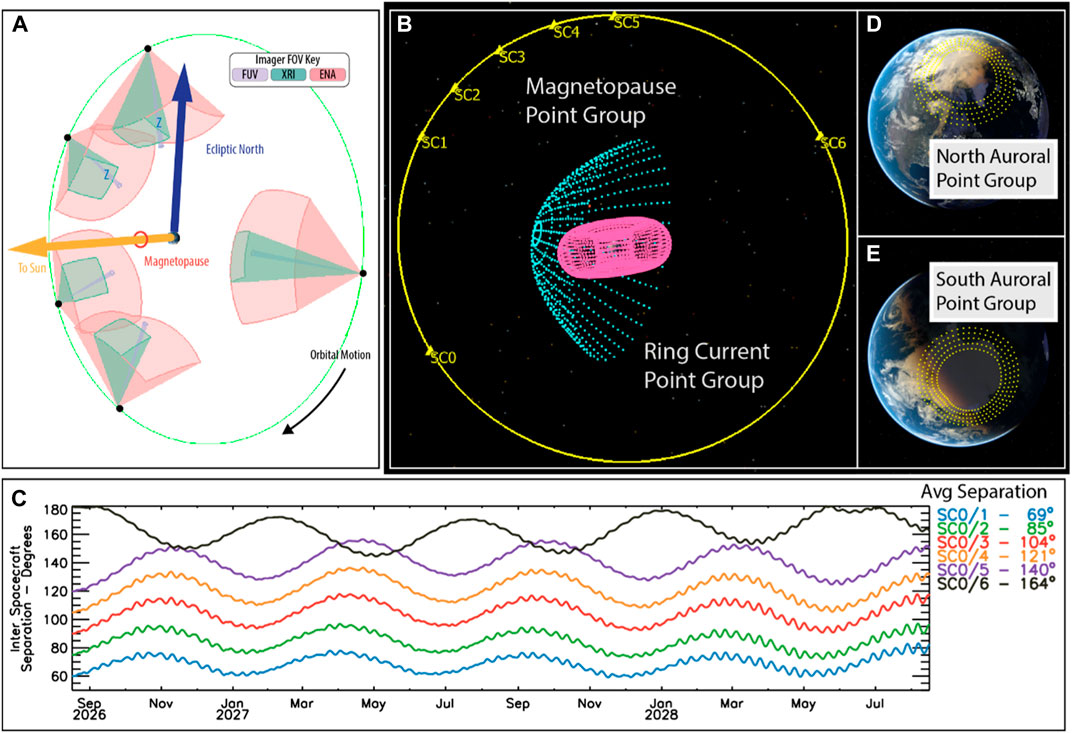
Figure 1. Overview of the STORM’s orbit and mission design. (A) STORM’s orbit during a period of high β-angle (orbital plane close to perpendicular to the sun-Earth line) and the fields-of-view of the FUV, XRI, and ENA imagers. (B) The phasing between a nominal single STORM spacecraft (SC0) and six potential secondary spacecraft (SC1-6) initially spaced at 60○, 75○, 90○, 105○, 120○, and 180○ along a shared orbit. Also illustrated are the magnetopause (teal) and ring current (pink) point groups used to define target and science visibility. (C) The variation in the spacecraft phasing throughout the two-year science mission as a result of external forces experienced by the spacecraft. The margin shows the average separation of each spacecraft with SC0 over the nominal two-year mission. (D) The northern and (E) southern hemisphere auroral point groups used to define the visibility of the auroral oval and auroral target and science visibility.
Panel (a) of Figure 1 illustrates STORM’s 30 RE circular orbit (9.65 day period), the spacecraft motion along the orbit, and the field of view of the XRI, FUV, and ENA imagers. The spacecraft orbit is based on the STORM mission design and Design Reference Mission (DRM), which assumed a nominal 30 RE circular orbit inclined 90○ to the ecliptic, with an August 2026 launch and insertion into science orbit in mid-August 2026 corresponding roughly with solar max of solar cycle 25. A spacecraft in such an orbit is perturbed strongly by the third-body gravitational effects from the Moon and Sun, which causes both periodic and secular changes to the orbital elements. The periodic changes include variations of approximately ±1○ in inclination. The eccentricity grows secularly over time (lowering perigee which eventually leads to atmospheric reentry) unless maintained by station-keeping maneuvers. Previous mission design efforts (Shoemaker et al., 2022) showed that a spacecraft in STORM’s orbit can maintain a 30 ± 1 RE radius orbit for up to 4 years without any station-keeping, even when perturbed by both natural (e.g., solar radiation pressure, third-body gravity) and manmade (e.g., momentum unload, science orbit insertion error) causes. For the string-of-pearls constellation of satellites assumed in the present study (Figure 1B), the individual spacecraft would be acted upon differently from one another by third-body gravitational effects (i.e., differential perturbation), such that their relative orbital changes over time cause their along-track separations to vary. Figure 1C shows the relative separation angle between each spacecraft and SC0, when the orbital dynamics are modeled with the gravitational effects from the Sun (point-mass), Moon (point-mass), Earth (10 × 10 spherical harmonics), and solar radiation pressure. The initial orbital state for each spacecraft is identical, aside from initial true anomaly (to give the phase angle separation) and the semi-major axis. The initial semi-major axis for SC1-6 was adjusted by several hundred km to achieve the relative angular separation profiles shown in Figure 1C. This initial configuration allows the along-track separation to be naturally maintained within approximately ± 15○ from a mean value over the two-year analysis span, without the need for active station keeping. Panels (b, d, and e) of Figure 1 show the position of six secondary spacecraft (labeled SC1 through six in panel b) and define the magnetopause, ring current, and north and south auroral point groups the represent STORM’s targets.
The point groups (Figure 1B, D, E) represent the physical location of the magnetopause, ring current, and aurora. The magnetopause point group is defined using the magnetopause shape from Sibeck et al. (1991) under nominal solar wind conditions. The ring current point group is defined by the surface of a toroid with inner and outer radius of 2.5 and 6.5 RE. The auroral point is defined as an elongated ellipse which encompasses the upper and lower limits of the auroral oval as observed by previous studies (e.g., Frey et al., 2004; Milan et al., 2009b; Milan et al., 2019). Together these point groups along with the FOV of the imagers are used to define when and what portion of the magnetopause, ring current, and auroral ovals are observed. This quantifies STORM’s target visibility. Coupled with a statistical analysis of historical solar and geomagnetic data this information is used to determine how often STORM can address each science objective, thus quantifying STORM’s science visibility. In the following section we describe the methodology used to define both target and science visibility and quantify the target and science visibility for each of STORM’s imagers and science objectives.
3 Target visibility
STORM’s target visibility is quantified through detailed analysis of the DRM, imager FOVs, and the point groups discussed in the previous section. STORM’s DRM simulates the spacecraft launch, insertion into the final 30 RE circular orbit, spacecraft motion along the orbit, orbit evolution and all spacecraft maneuvers through a nominal two-year mission. The DRM also fully models the spacecraft including the position of each instrument, the spacecraft attitude, and the FOVs of the imagers and thus models in a precise way what fraction of each point group the corresponding imager is able to observe at any given point throughout the mission. Specifically, for each point group, we use a binary classification which labels a point as inside the FOV of an imager (1) or outside the FOV of the imager (0). When considering coincident observation by two spacecraft a point is classified as observed if it is in the FOV of an imager on either spacecraft. This is done for the entirety of a nominal 2-year mission at 1 h cadence (the cadence of the DRM). The ratio of observed points labeled with a ‘1’ to the total number of points within a point group is the fraction of the point group observed by an imager at any given point in time.
For the magnetopause, we define a subset of the point group which encompasses the magnetopause nose as our target. This is because the motion of the magnetopause nose is a key observable for addressing several of STORM’s science objectives (Sibeck et al., 2023a). The larger point group, while not used in subsequent analysis, is useful for quantifying target and science visibility of potential secondary objectives such as the dynamics of the Kelvin-Helmholtz stability along the magnetopause flanks. For the ring current we consider the entirety of the torus point group shown in Figure 1B. For the aurora, the two point covering the northern and southern auroral oval, are each subdivided by clock-angle into four subgroups which define dayside, dusk, night-side, and dawn auroral point groups. Additional statistics are composed by combining the north and south auroral point groups into a single auroral point group that can be observed regardless of the hemisphere. For the magnetopause nose and auroral point groups, if 98% of the points are observed we define those targets as being visible. For the ring current point group if 95% of the point group is observed the target is defined as visible. These, extremely conservative, thresholds are set so that if a small number of points on the edges of the point group are not visible, we do not define the target as not being visible.
Figure 2 shows the results of the target visibility analysis for a single spacecraft STORM mission (SC0 in Figure 1B) through the initial 6 months of a nominal science phase. In this initial 6-month period the STORM spacecraft visits all magnetic local times. The target visibility is calculated at the hourly cadence of DRM. Evident in Figure 2 is that ENA has the largest target visibility, followed by XRI, and the FUV. This is not surprising as ENA’s observations of the ring current are rarely impeded, and most visibility dropouts result from spacecraft sun-avoidance maneuvers required to keep the sun out of the FOV of the imagers. XRI has the second highest visibility through the 6-month period. XRIs target, the magnetopause nose, can be impeded by the Earth throughout various portions of STORM’s orbit, for example, when the spacecraft is on the night side. As expected FUV has the lowest target visibility since twice during every 9.65 day orbit the STORM spacecraft is in or near the equatorial place where FUV is unable to observe the high-latitude aurora.
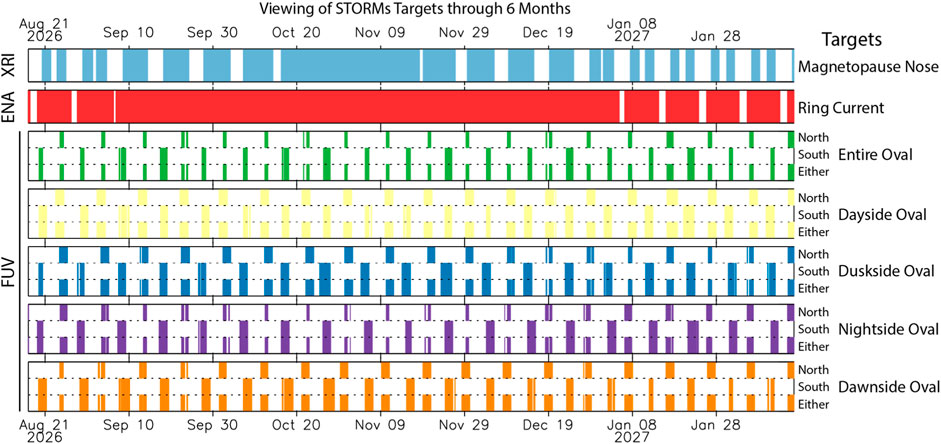
Figure 2. Target visibility of each of STORM’s key observables. From top to bottom, the magnetopause nose (observed by XRI), the ring current (observed by ENA), the auroral oval and its four sectors, day, dusk, night, and dawn (observed by FUV). Note the auroral oval target visibility is broken down by hemisphere and also further combined to show visibility regardless of hemisphere.
Figure 3 expands on the analysis of Figure 2 and the number of hours each target can be observed over the entirety of a two-year science mission for a single STORM spacecraft (SC0) and each paired combination of SC0 and SC1 through SC6. Over the course of a two-year mission a single STORM spacecraft observes the magnetopause nose for over 11,000 h; the ring current for over 15,000 h; the auroral oval for nearly 2000 h; and the four sectors of the aurora oval for nearly 3,000 h each. For a dual spacecraft mission the hours of observing the ring current slightly increase and remains relatively constant for any spacecraft pair. Observations of the magnetopause increase significantly with a dual spacecraft mission. This is because with two spacecraft, the number of times when neither can observe magnetopause is drastically reduced. For auroral observations, the addition of a second spacecraft nearly doubles the total number of hourly intervals when an auroral target can be observed. For the four auroral sectors the number of hourly target visibility intervals peaks for SC0 and SC2 which are separated on average by 85○. For the full auroral oval, target visibility peaks for SC0 and SC1 which are separated by an average 69○.
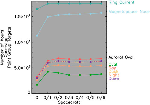
Figure 3. Target visibility for each of STORM’s targets for a single spacecraft mission and six potential dual spacecraft missions (x-axis).
In the following section we combine the target visibility derived here with a statistical analysis of solar wind and geomagnetic observations during solar cycles 23 and 24 to quantify STORM’s science visibility for each objective. That is, how many hourly intervals exist when STORM observes the necessary targets during appropriate solar wind and geomagnetic conditions so that the science objectives can be addressed.
4 Science visibility
STORM’s science visibility builds on the analysis which quantified the target visibility to provide a detailed statistical estimation of the number of hourly intervals during which STORM can address each of its four science objectives. This is accomplished by first identifying the necessary solar wind, magnetosphere, and geomagnetic thresholds required to address a specific mission objective. A synthetic time series of these solar wind, magnetosphere, and geomagnetic variables is then generated using historical data that has been epoch-advanced to mimic the solar cycle phase we believe STORM will be launched during. This synthetic time-series is combined with the target visibility to quantify when and how often specific thresholds are met or exceeded such that a science objective can be addressed. Specific thresholds include, for instance, the onset of a geomagnetic substorm or storm or an enhanced southward interplanetary magnetic field which can initiate dayside reconnection.
As an example, we can consider science objective A–Energy Transfer at the Dayside Magnetopause. As part of objective A STORM will use the XRI and FUV instruments to determine how dayside reconnection controls the flow of solar wind energy into the magnetosphere and the spatial and temporal properties of this interaction as a function of solar wind conditions (Sibeck et al., 2023a). To address these two questions XRI must observe the magnetopause nose and FUV must observe the dayside auroral oval during periods of elevated solar wind flux and southward IMF (Sibeck et al., 2023a). Here we use a threshold solar wind flux (SWF) of 2.5 × 108 cm-2s-1 and southward IMF of 5 nT (or −5 nT Bz). These solar wind thresholds allow XRI to track the motion of the magnetopause driven by reconnection at cadence sufficient to distinguish bursty reconnection from fast/slow steady reconnection (Sibeck et al., 2018; Sibeck et al., 2023a) and FUV to track proton auroral precipitation associated with magnetopause reconnection (Frey et al., 2002).
Figure 4 shows the culmination of this analysis using synthetic solar wind data from solar cycle 24 over a nominal two-year science mission. Panels (a) and (b) show the target visibility of the magnetopause nose and dayside auroral oval (c.f., Figure 1), and panel (c) shows when the two target visibilities overlap. Panels (d) and (e) show the synthetic IMF Bz and SWF time series during a two-year period around solar max of solar cycle 24 from the 1-h OMNI dataset (King and Papitashvili, 2005). We use a two-year period around solar max as this would be the nominal launch window and science mission phase of STORM. In panels (d) and (e) the dashed lines show the IMF Bz and solar wind flux thresholds. In panel (d) the circles identify hourly periods when IMF Bz exceeds its threshold and the FUV instrument can observe the dayside auroral oval. In panel (e) the circles identify when both IMF Bz and solar wind flux exceed their respective thresholds and the XRI instrument can observe the magnetopause nose. The text in the right margin of Figure 4 summarizes the total number of target visibility hours, and science target visibility hours for objective A.
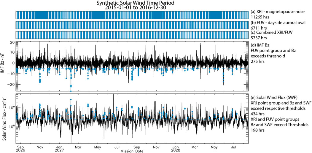
Figure 4. Target and science visibility for Objective A through a nominal two-year mission. (A–C) The target visibility of the magnetopause, dayside auroral oval, and times when both targets can be observed by STORM. (D, E) the synthetic IMF and solar wind flux time series used to define the science criteria for Objective A, the dashed lines show the thresholds of −5 nT and 2.5 × 108 cm-2s-1. The circles indicate times when the thresholds are exceeded and the target can be observed, these are periods of science visibility. The text in the margin summarizes the target and science visibility for Objective A.
The analysis shown in Figure 4 provides a single estimate of the number of science visibility hours for Objective A quantified from a two-year synthetic solar wind time series taken from historical data. However, the solar wind is quite variable such that the estimated science visibility can change based on the two-year time period selected, where within the solar cycle the synthetic timeseries came from and from what solar cycle. To account for this variability, we use a k-folds or Monte Carlo framework which allows us to statistically estimate the science visibility as well as provide error bounds on this estimate. In short, ten synthetic solar wind timeseries are randomly sampled from a specified time interval. For each of these synthetic timeseries the science visibility is quantified as in Figure 4. The average and standard deviation of the mean of these ten estimates are then used to provide an overall estimate and error in the estimate of the science visibility.
Nominally STORM will launch around solar max, thus for this analysis we consider two-time intervals, solar max of solar cycle 23 and solar max of solar cycle 24. The max of solar cycle 23 and 24 are defined as 2000-03-03 and 2014-01-01 which lie close to the peak number of sunspots during each solar cycle. From these dates ten random time shifts of ±1 year are applied producing ten synthetic time series around the max of solar cycle 23 and 24 which are then used to complete the k-folds analysis. Figure 5 summarizes this k-folds analysis for science visibility for objective A for a single spacecraft mission and potential dual spacecraft missions. There are a larger number of hourly science visibility observing intervals during solar cycle 23 than solar cycle 24. This is not surprising as solar cycle 24 was unusually quiet. Science visibility also peaks for the SC0/2 dual spacecraft mission, consistent with the peak in target visibility in Figure 3. Important to note though is that there are several hundreds of hours of science visibility during solar cycle 24 to address science objective A with a single spacecraft mission even during an unusually quiet solar cycle.
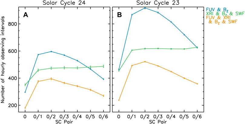
Figure 5. Science visibility for Objective A during (A) solar cycle 24 and (B) solar cycle 23. Blue–FUV observes dayside aurora and Bz < −5 nT; green XRI observes the magnetopause nose and Bz < −5 nT and SWF > 2.5 × 108 cm-2s-1; orange FUV observes dayside aurora, XRI observes magnetopause nose, and Bz < −5 nT and SWF > 2.5 × 108 cm-2s-1.
STORM addresses its overall science goal by addressing the four objectives described in Section 2 Mission Concept. A detailed description of these science objectives, background regarding unanswered questions, how STORM distinguished between proposed interaction modes, determines occurrence patterns for each mode, and quantifies the significance of each mode, as well as the measurement requirements to address each objective and the dynamics of each mode were given by Sibeck et al. (2023a). Table 1 summarizes these details for each objective and identifies the physical process STORM is investigating, and the required instrument, target, and solar wind and/or geomagnetic conditions necessary to study that process. These identified instruments, targets, and solar wind and/or geomagnetic conditions are used to quantify the science visibility for each of STORM’s objectives in the same way as for the detailed example for Objective A presented above. The same data set that was used for Objective A is used to generate a list of geomagnetic storms through solar cycles 23 and 24 using the methodology outlined in Murphy et al. (2018). This storm list is used to define an additional synthetic time series that separates all times into storm-times or quiet-times and further subdivides storm-times into either main phase or recovery phase. To generate a time-series of synthetic substorm onsets we use the Newell and Gjerloev (2011) substorm list through solar cycle 23 and 24 and tag each hour as either having or not having a substorm onset. This binary time-series is used to generate a synthetic time-series of whether a substorm onset occurs during any hour of the nominal two-year science mission. Figures 5–8 show the results of the science visibility and k-folds analysis for each objective and physical process detailed in Table 1.
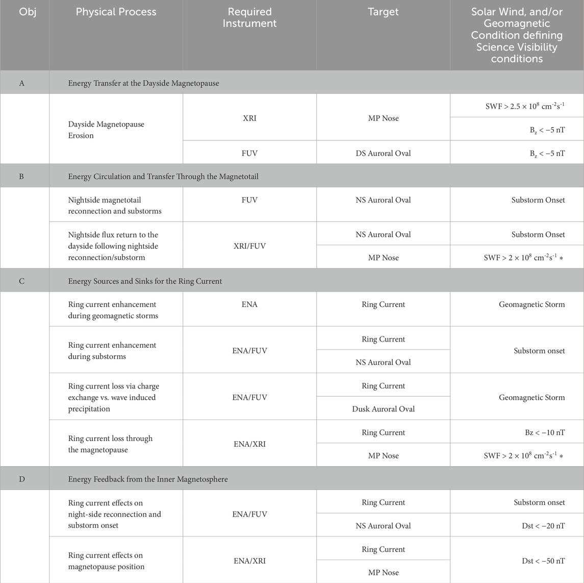
Table 1. Summary of the physical processes, required instrument, target, and solar wind and geomagnetic conditions required to address each of STORM’s four science objectives. * A lower SWF threshold is required as these ojbectives can be addressed using XRI with a lower cadence then required for Objective A.
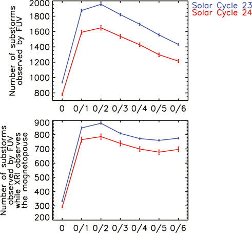
Figure 6. Science visibility for STORM’s Objective (B) (A) The number of substorms observed by FUV and (B) the number of substorms observed by FUV when XRI observes the magnetopause nose for single and dual spacecraft missions (x-axis). The science visibility is estimated from both solar cycle 23 and 24 (blue and red).
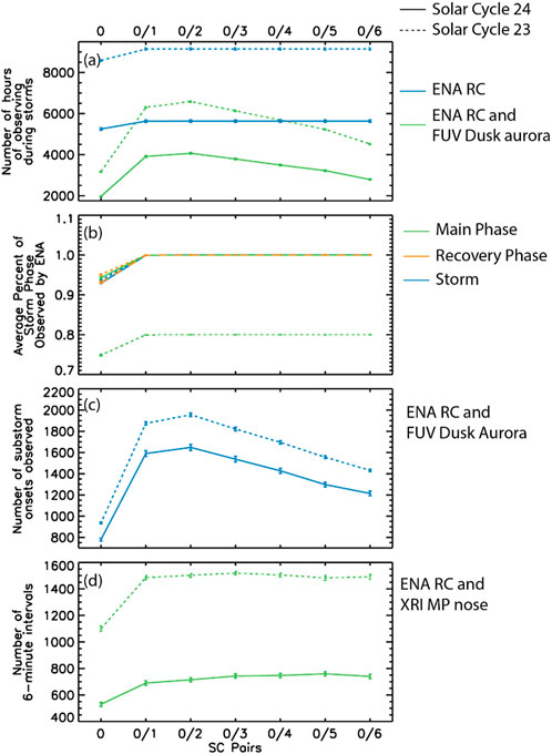
Figure 7. Science visibility for STORM’s Objective C during solar cycle 23 (dashed) and 24 (solid) for a single and dual spacecraft mission (x-axis). (A) Number of hours observing the ring current (blue) and ring current/dusk auroral oval (green). (B) Percentage of storm (blue) and storm main (green) and recovery (orange) phases that ENA observes the ring current. (C) Number of substorms during an enhanced ring current when FUV can observe substorm onset and ENA can observed the ring current. (D) Number of 6-min intervals during an enhanced ring current when the ring current and magnetopause nose can be observed.
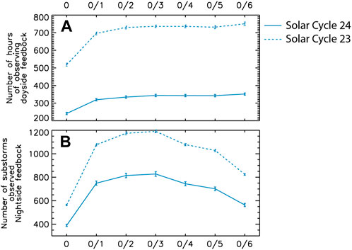
Figure 8. Science visibility for STORM’s Objective D estimated from solar cycle 23 (dashed) and 24 (solid) as a function of single and dual spacecraft mission configurations (x-axis). (A) The number of hourly intervals when STORM can investigate inner-magnetosphere feedback on the dayside magnetopause. (B) The number of substorm during which STORM can investigate feedback of the inner magnetosphere on nightside reconnection and substorm dynamics.
Figure 6 shows the science visibility of Objective B Energy Circulation and Transfer Through the Magnetotail. This is achieved by determining how magnetotail reconnection regulates the circulation of energy from the dayside, through the magnetotail, and into the inner magnetosphere (Dungey, 1961) and by quantifying the occurrence and significance of differing reconnection modes (Sibeck et al., 2023a). In the tail, night side reconnection is the physical mechanism releasing stored energy. This energy is released by the onset of a substorm and localized brightening of the aurora. Subsequently, and depending on the solar wind and magnetosphere conditions this auroral brightening and substorm can evolve into a set of sawtooth substorms or extended periods of steady magnetospheric convection (DeJong et al., 2007; 2009). If the auroral brightening is localized the mode is characterized as a pseudo-breakup, a substorm like event where tail reconnection is believed to quenched or limited (Rostoker, 1998). Substorms, pseudo-breakups, sawtooth events, and steady magnetosphere convection are the different tail reconnection modes STORM will study to address Objective B. To do this STORM must observe substorm onsets with FUV so that the drivers of these various modes can be identified (c.f., Sibeck et al., 2023a). Coupled with XRI, FUV observations of these modes can further be used to determine how and whether these different tail reconnection modes return magnetic flux to the dayside magnetosphere (Dungey, 1961; Dungey, 1961). The top panel of Figure 6 shows the number of substorms that STORM FUV will observe in both single and dual-spacecraft configurations. The bottom panel shows the subset of these substorms during which XRI can also observe the magnetopause nose and hence flux returned to the dayside magnetopause. As with Objective A, the peak in science visibility of Objective B occurs for the SC0/2 spacecraft pair and the science visibility is higher during the more active solar cycle 23. Of note is that a single spacecraft mission observes a significant number of substorms on its own; ∼800 with FUV and ∼300 with both FUV and XRI.
STORM’s Objective C will follow the energy released from magnetotail reconnection into the inner magnetosphere to quantify the sources and sinks and of ring current energization. To quantify the source of ring current energy, STORM must observe the ring current during geomagnetic storms and substorms, periods of ring current energization (Sibeck et al., 2023a). To quantify the sinks of ring current energy, including charge exchange, precipitation driven by wave-particle interactions (e.g., electromagnetic ion cyclotron waves, EMIC, etc.), and direct loss through the magnetosphere, STORM must observe the dusk side auroral oval in combination with an enhanced ring current (e.g., geomagnetic storm periods), and the magnetopause boundary in combination with an enhanced ring current. These observations will allow STORM to initially determine the dominant sink of ring current energy and subsequently quantify the relative efficiency of the three sinks (c.f., Figure 6; Sibeck et al., 2023b). Figure 7 shows the science visibility for each of these scenarios. Panels (a) and (b) of Figure 7 quantify STORM’s science visibility during geomagnetic storms. Panel (a) depicts the number of hours ENA observes the ring current (ring current dynamics during storms) and the subset of these periods when FUV also observes the dusk side auroral oval (EMIC wave driven ring current loss). Panel (b) shows the average percentage of a geomagnetic storm, and the storm main and recovery phases where ENA observes the ring current. A single spacecraft STORM mission observes a significant number (∼2000) of hourly intervals during geomagnetic storms. This roughly doubles for a dual spacecraft mission. In terms of “how much of a geomagnetic storm can be observed?” this is generally above 90%, that is ENA can observe the ring current for 90% of storms and storm main or recovery phases. Panel (c) shows the number of hourly intervals ENA observes the ring current and FUV observes the night-side auroral oval and a substorm occurs (substorm energization of the ring current). A single spacecraft mission observes ∼800-1,000 substorms and a dual spacecraft mission observes as many as ∼1,600-2000 substorms, depending on the solar cycle. Finally, panel (d) shows the number of 6-min intervals during which XRI observes the magnetopause nose, ENA observes the ring current, and the IMF Bz < −10 nT and SWF > 2 × 108 cm-2s-1. The increased Bz threshold is necessary for the magnetopause to penetrate the inner magnetosphere (Staples et al., 2022) such that ring current loss through the magnetopause may be quantified; the number of intervals peaks for a dual spacecraft mission but remains high with ∼500 and ∼1,500 intervals for solar cycle 24 and 23, respectively.
Objective C investigates the dynamics of the energization of the inner magnetosphere; however, it is also important to consider the effects that the inner magnetosphere can have on other plasma systems. In particular a strong storm-time ring current may affect the position of the magnetopause (Tsyganenko and Sibeck, 1994; García and Hughes, 2007; Samsonov et al., 2016) and the latitude of substorm onset and the amount of open flux required to initiate tail reconnection (Milan et al., 2009a). Objective D will investigate energy feedback from the inner magnetosphere and the effects a strong ring-current has on the day and nightside magnetosphere. To investigate ring current feedback on the magnetopause XRI must observe the magnetopause nose, as ENA observes an enhanced ring current, defined here as Dst < −50 nT. These parameters define the science visibility for ring current feedback on the dayside magnetosphere which is shown in Figure 8 panel (a). To investigate the effect that the ring current has on nightside reconnection requires observations of an enhanced ring current with varying intensities and substorms onset. To achieve this the science visibility requires ENA to observe an enhanced ring current, defined as periods when Dst < -20 nT, and FUV must observe the nightside auroral oval during a substorm. This science visibility is shown in Figure 8 panel (b). Note the difference in the Dst thresholds for these two science visibilities, different thresholds were specifically chosen as it is postulated that a larger ring current is required to affect the dayside magnetopause due to larger magnetic field strengths at the magnetopause then in the night-side tail during periods of extreme tail stretching observed before substorm onset. Overall, STORM has a significant number of events to address Objective D, with a minimum of ∼200 h to address dayside feedback and ∼400 substorms to address nightside feedback, both during periods when the ring current is enhanced. As with the other objectives, more events are observed for solar cycle 23 then solar cycle 24, and for a dual spacecraft mission consisting of SC0 and 2. In the next section we provide a brief summary of the results presented here and perspective looking forward to the future.
5 Summary and perspective
Earth Science, Heliophysics, and Astrophysics imaging missions have enabled fundamental scientific advances. In Earth Science, the advent of scientific imaging transformed meteorology. For example, the Geostationary Operational Environmental Satellite (GOES) family of satellites have provided continuous and reliable environmental information used to support weather forecasting, storm tracking, and research (Hawkings et al., 1996). The importance of such observations was demonstrated during the GOES I-M era with the successful tracking and monitoring of hurricanes Hugo and Andrew (Hawkings et al., 1996). In Astrophysics, imagers and telescopes have been the corner stone of scientific research for centuries. Following the space age, space-borne telescopes have been used characterize the cosmic microwave background (Hinshaw et al., 2013), study the aurora on other planets (Clarke et al., 1998), and identify exoplanets (Borucki, 2016). In solar physics, imagers are commonly used to monitor activity on the sun and its relation to space weather (Darnel et al., 2022) and for scientific research, including the Solar TErrestrial RElations Observatory (STEREO) mission designed to capture stereographic images of coronal mass ejections (Kaiser et al., 2008). In magnetospheric physics, imaging has been used to study the auroral (Mende, 2016), ring current (Brandt, 2002), and plasmaspheric (Goldstein et al., 2003) dyanmics. These observations have provided fundamental insight into solar wind-magnetosphere coupling, linking dayside reconnection to auroral precipitation (Frey et al., 2003), and inner-magnetospheric dynamics, via stereographic images of the terrestrial ring current (Goldstein and McComas, 2018).
This paper detailed the target and science visibility of the Solar-Terrestrial Observer for the Response of the Magnetosphere (STORM) mission concept. STORM’s overarching science goal is to study the system science of and flow of energy in the solar wind-magnetosphere system. STORM achieves this by observing key plasma regimes and systems associated with the Dungey cycle and coupled solar wind-magnetosphere system. This is referred to as STORM’s target visibility, how often a specific target can be observed, and is illustrated in Figures 3, 4. STORM’s science visibility quantifies the number of intervals (typically hourly intervals) when STORM can address its science objectives and overarching science goal, e.g., when the solar and geomagnetic conditions are sufficient to conduct science. This science visibility is derived for a single spacecraft and six spacecraft pairs which could form a potential dual spacecraft mission (c.f., Figure 1B). These target and science visibility was determined through a detailed analysis of the Design Reference Mission (DRM), instrument FOVs, and target locations, combined with a statistical analysis of historical solar wind conditions during solar cycles 23 and 24 (an active and quiet solar cycle). The analysis demonstrating how the science visibility is quantified is illustrated in Figures 4, 5; Figures 5–8 show the science visibility for each of STORM’s four science objectives (Section 2—Mission Concept).
Overall, Figure 3 demonstrates that STORM observes each of its required targets, the magnetopause, the auroral oval and dusk, dawn, day, and night sectors, and the ring current for significant portions of the mission. The auroral oval is observed for a minimum of 2000 h and increases to ∼3,000 h for each sector. The magnetopause is observed for a minimum of ∼11,000 h and the ring current a minimum of ∼16,000 h. These numbers increase for a dual spacecraft mission and peak for the SC0/2 pair, which are on average 85○ out of phase (in a shared orbit Figure 1B). Regarding science visibility (Figures 5–8), STORM has several hundreds of intervals to address each of its objectives with a single spacecraft. The science visibility is larger during solar cycle 23 than 24, which is not surprising given the subdued nature of solar cycle 24 (Basu, 2013). Like STORMs target visibility, the science visibility peaks (in general) for spacecraft pair SC0/2 and provides the largest number of observations of the aurora and its four sectors which subsequently also creates a peak in the science visibility.
It is important to remind the reader that a statistical analysis of historical solar wind data around solar max of solar cycles 23 and 24 was used to quantify and estimate an error in the science visibility for each objective. This was done using a k-folds or Monte Carlo technique (described in Section 4—Target Visibility). This statistical analysis was performed to account for the non-normal and non-periodic distribution of solar wind and geomagnetic conditions required to address STORM’s science and gives a more accurate representation of the science visibility then assuming a fixed distribution of events. For example, the rate of geomagnetic storms peaks during solar max; however, geomagnetic storms are not periodic and do not occur with a fixed frequency. The k-folds/Monte Carlo technique accounts for this and provides a more robust estimation of the expected science visibility and its errors (or variation–see Section 4 for details). Of note are the errors in the science visibility shown in Figures 5–8. They are small compared to the estimated science visibility, such that, in general, the science visibility does not vary significantly when considering a two-year period around solar max, which may potentially shift forward or backward by up to a year. There is larger variation in science visibility as a function of solar cycle and there is likely to be variation with solar phase. However, STORM would nominally launch around solar max and so the science visibility was calculated for that period of the solar cycle. Finally, both solar cycle 23 and 24 were used to determine science visibility in order to provide an upper and lower estimate from an active and quiet solar cycle.
In short, a single spacecraft STORM mission launched during a quiet solar cycle has a significant number of science visibility intervals. This would provide hundreds of intervals to address STORM’s overarching science goals and each of the four science objectives allowing researchers to conduct case studies of particular events as well as statistical studies to determine the spatial and temporal characteristics of the fundamental phenomena coupling the solar wind and magnetosphere and leading the redistribution of energy throughout the magnetosphere. A dual spacecraft mission significantly increases science visibility and allows for stereographic imaging and tomography (see Cucho-Padin et al. this issue) which a single spacecraft can only do statistically. However, a dual spacecraft mission would significantly increase the overall complexity and budget as compared to a single spacecraft mission. Without a target budget value it is impossible to settle on a final STORM design, single vs. dual spacecraft. Recent NASA Medium Class Explore (MIDEX) announcements of opportunity have had budgets which align with a single STORM spacecraft mission and would allow STORM to fully address its objectives. However, if budgets increase it may be possible to consider a dual spacecraft mission and investigate the three-dimensional structure and dynamics of magnetopause and ring current via tomographic techniques, while observing STORM’s targets for significant periods of time. Regardless, STORM would be the first stand-alone and complete system science mission capable of studying the end-to-end dynamics of the coupled solar wind-magnetosphere system and resulting flow of energy in the Dungey cycle (Sibeck et al., 2023b).
Data availability statement
The raw data supporting the conclusion of this article will be made available by the authors, without undue reservation.
Author contributions
KM: Conceptualization, Data curation, Formal Analysis, Funding acquisition, Investigation, Methodology, Project administration, Resources, Software, Supervision, Validation, Visualization, Writing–original draft, Writing–review and editing. MS: Conceptualization, Formal Analysis, Investigation, Methodology, Software, Visualization, Writing–original draft, Writing–review and editing. DS: Conceptualization, Methodology, Resources, Visualization, Writing–original draft, Writing–review and editing. CS: Conceptualization, Investigation, Methodology, Visualization, Writing–original draft, Writing–review and editing. HC: Conceptualization, Investigation, Methodology, Visualization, Writing–original draft, Writing–review and editing. FP: Conceptualization, Investigation, Methodology, Visualization, Writing–original draft, Writing–review and editing. EZ: Conceptualization, Formal Analysis, Investigation, Methodology, Visualization, Writing–original draft, Writing–review and editing.
Funding
The author(s) declare that financial support was received for the research, authorship, and/or publication of this article. This work is supported in part by a NASA GSFC IRAD.
Conflict of interest
The authors declare that the research was conducted in the absence of any commercial or financial relationships that could be construed as a potential conflict of interest.
Publisher’s note
All claims expressed in this article are solely those of the authors and do not necessarily represent those of their affiliated organizations, or those of the publisher, the editors and the reviewers. Any product that may be evaluated in this article, or claim that may be made by its manufacturer, is not guaranteed or endorsed by the publisher.
References
Basu, S. (2013). The peculiar solar cycle 24 – where do we stand? J. Phys. Conf. Ser. 440, 012001. doi:10.1088/1742-6596/440/1/012001
Borovsky, J. E., and Valdivia, J. A. (2018). The Earth’s magnetosphere: a systems science overview and assessment. Surv. Geophys. 39 (5), 817–859. doi:10.1007/s10712-018-9487-x
Borucki, W. J. (2016). KEPLER Mission: development and overview. Rep. Prog. Phys. 79 (3), 036901. doi:10.1088/0034-4885/79/3/036901
Brandt, P. C., Mitchell, D. G., Ebihara, Y., Sandel, B. R., Roelof, E. C., Burch, J. L., et al. (2002). Global IMAGE/HENA observations of the ring current: examples of rapid response to IMF and ring current-plasmasphere interaction. J. Geophys. Res. 107 (A11), 1359. doi:10.1029/2001JA000084
Clarke, J. T., Ballester, G., Trauger, J., Ajello, J., Pryor, W., Tobiska, K., et al. (1998). Hubble Space Telescope imaging of Jupiter’s UV aurora during the Galileo orbiter mission. J. Geophys. Res. Planets 103 (E9), 20217–20236. doi:10.1029/98JE01130
Darnel, J. M., Seaton, D. B., Bethge, C., Rachmeler, L., Jarvis, A., Hill, S. M., et al. (2022). The GOES-R solar UltraViolet imager. Space weather. 20 (4). doi:10.1029/2022SW003044
DeJong, A. D., Cai, X., Clauer, R. C., and Spann, J. F. (2007). Aurora and open magnetic flux during isolated substorms, sawteeth, and SMC events. Ann. Geophys. 25 (8), 1865–1876. doi:10.5194/angeo-25-1865-2007
DeJong, A. D., Ridley, A. J., Cai, X., and Clauer, C. R. (2009). A statistical study of BRIs (SMCs), isolated substorms, and individual sawtooth injections. J. Geophys. Res. Space Phys. 114 (A8). doi:10.1029/2008JA013870
Dungey, J. W. (1961). Interplanetary magnetic field and the auroral zones. Phys. Rev. Lett. 6 (2), 47–48. doi:10.1103/PhysRevLett.6.47
Frey, H. U., Meade, S. B., Immel, T. J., Fuselier, S. A., Claflin, E. S., Gérard, J.-C., et al. (2002). Proton aurora in the cusp. J. Geophys. Res. 107 (A7), 1091. doi:10.1029/2001JA900161
Frey, H. U., Mende, S. B., Angelopoulos, V., and Donovan, E. F. (2004). Substorm onset observations by IMAGE-FUV. J. Geophys. Res. 109 (A10), A10304. doi:10.1029/2004JA010607
Frey, H. U., Phan, T. D., Fuselier, S. A., and Mende, S. B. (2003). Continuous magnetic reconnection at Earth’s magnetopause. Nature 426 (6966), 533–537. doi:10.1038/nature02084
García, K. S., and Hughes, W. J. (2007). Finding the Lyon-Fedder-Mobarry magnetopause: a statistical perspective. J. Geophys. Res. Space Phys. 112 (A6). doi:10.1029/2006JA012039
Goldstein, J., and McComas, D. J. (2018). The big picture: imaging of the global geospace environment by the TWINS mission. Rev. Geophys. 56 (1), 251–277. doi:10.1002/2017RG000583
Goldstein, J., Sandel, B. R., Forrester, W. T., and Reiff, P. H. (2003). IMF-driven plasmasphere erosion of 10 July 2000. Geophys. Res. Lett. 30 (3), 1146. doi:10.1029/2002gl016478
Gombosi, T. I., Chen, Y., Glocer, A., Huang, Z., Jia, X., Liemohn, M. W., et al. (2021). What sustained multi-disciplinary research can achieve: the space weather modeling framework. J. Space Weather Space Clim. 11, 42. doi:10.1051/swsc/2021020
Hawkings, J., Staton, C. P., Paquett, J. A., Barbieri, L. P., Suranno, M. A., Reynolds, R., et al. (1996) GOES I-M databook.
Hinshaw, G., Larson, D., Komatsu, E., Spergel, D. N., Bennett, C. L., Dunkley, J., et al. (2013). Nine-year wilkinson microwave anisotropy probe (wmap) observations: cosmological parameter results. Astrophysical J. Suppl. Ser. 208 (2), 19. doi:10.1088/0067-0049/208/2/19
Kaiser, M. L., Kucera, T. A., Davila, J. M., St. Cyr, O. C., Guhathakurta, M., and Christian, E. (2008). The STEREO mission: an introduction. Space Sci. Rev. 136 (1–4), 5–16. doi:10.1007/s11214-007-9277-0
Kepko, L. (2018). “Magnetospheric constellation: leveraging space 2.0 for big science,” in Igarss 2018 - 2018 IEEE international geoscience and remote sensing symposium, 285–288. doi:10.1109/IGARSS.2018.8519475
King, J. H., and Papitashvili, N. E. (2005). Solar wind spatial scales in and comparisons of hourly Wind and ACE plasma and magnetic field data. J. Geophys. Res. 110 (A2), A02104. doi:10.1029/2004JA010649
Lin, D., Sorathia, K., Wang, W., Merkin, V., Bao, S., Pham, K., et al. (2021). The role of diffuse electron precipitation in the formation of subauroral polarization streams. J. Geophys. Res. Space Phys. 126 (12). doi:10.1029/2021JA029792
Lin, Y., Duan, X., Zhao, C., and Xu, L.Da. (2012) Systems science. Boca Raton: CRC Press. doi:10.1201/b13095
Mende, S. B. (2016). Observing the magnetosphere through global auroral imaging: 2. Observing techniques. J. Geophys. Res. Space Phys. 121 (10), 10,638–10,660. doi:10.1002/2016JA022607
Milan, S. E., Grocott, A., Forsyth, C., Imber, S. M., Boakes, P. D., and Hubert, B. (2009a). A superposed epoch analysis of auroral evolution during substorm growth, onset and recovery: open magnetic flux control of substorm intensity. Ann. Geophys. 27 (2), 659–668. doi:10.5194/angeo-27-659-2009
Milan, S. E., Hutchinson, J., Boakes, P. D., and Hubert, B. (2009b). Influences on the radius of the auroral oval. Ann. Geophys. 27 (7), 2913–2924. doi:10.5194/angeo-27-2913-2009
Milan, S. E., Walach, M.-T., Carter, J. A., Sangha, H., and Anderson, B. J. (2019). Substorm onset latitude and the steadiness of magnetospheric convection. J. Geophys. Res. Space Phys. 124 (3), 1738–1752. doi:10.1029/2018JA025969
Murphy, K. R., Watt, C. E. J., Mann, I. R., Jonathan Rae, I., Sibeck, D. G., Boyd, A. J., et al. (2018). The global statistical response of the outer radiation belt during geomagnetic storms. Geophys. Res. Lett. 45 (9), 3783–3792. doi:10.1002/2017GL076674
Newell, P. T., and Gjerloev, J. W. (2011). Evaluation of SuperMAG auroral electrojet indices as indicators of substorms and auroral power. J. Geophys. Res. Space Phys. 116 (A12). doi:10.1029/2011JA016779
Rostoker, G. (1998). On the place of the pseudo-breakup in a magnetospheric substorm. Geophys. Res. Lett. 25 (2), 217–220. doi:10.1029/97GL03583
Samsonov, A. A., Gordeev, E., Tsyganenko, N. A., Šafránková, J., Němeček, Z., Šimůnek, J., et al. (2016). Do we know the actual magnetopause position for typical solar wind conditions? J. Geophys. Res. A Space Phys. 121 (7), 6493–6508. doi:10.1002/2016JA022471
Shoemaker, M. A., Folta, D. C., and Sibeck, D. G. (2022). “Application of tisserand’s criterion and the lidov-kozai effect to STORM’s trajectory design,” in AAS/AIAA astrodynamics specialist conference.
Sibeck, D. G., Allen, R., Aryan, H., Bodewits, D., Brandt, P., Branduardi-Raymont, G., et al. (2018). Imaging plasma density structures in the soft X-rays generated by solar wind charge exchange with neutrals. Space Sci. Rev. 214 (4), 79. doi:10.1007/s11214-018-0504-7
Sibeck, D. G., Lopez, R. E., and Roelof, E. C. (1991). Solar wind control of the magnetopause shape, location, and motion. J. Geophys. Res. 96 (A4), 5489. doi:10.1029/90JA02464
Sibeck, D. G., Murphy, K. R., Porter, F. S., Connor, H. K., Walsh, B. M., Kuntz, K. D., et al. (2023a). Quantifying the global solar wind-magnetosphere interaction with the Solar-Terrestrial Observer for the Response of the Magnetosphere (STORM) mission concept. Front. Astronomy Space Sci. 10. doi:10.3389/fspas.2023.1138616
Sibeck, D. G., Murphy, K. R., Porter, F. S., Walsh, B., Connor, H., Kuntz, K., et al. (2023b). Imaging the end-to-end dynamics of the global solar wind-magnetosphere interaction. Bull. AAS. doi:10.3847/25c2cfeb.9b87eed9
Staples, F. A., Kellerman, A., Murphy, K. R., Rae, I. J., Sandhu, J. K., and Forsyth, C. (2022). Resolving magnetopause shadowing using multimission measurements of phase space density. J. Geophys. Res. Space Phys. 127 (2), e2021JA029298. doi:10.1029/2021JA029298
Keywords: imaging, dungey cycle, magnetosphere, solar wind, reconnection, system science, dual spacecraft
Citation: Murphy KR, Shoemaker MA, Sibeck DG, Schiff C, Connor H, Porter FS and Zesta E (2024) Target and science visibility of the solar-terrestrial observer for the response of the magnetosphere (STORM) global imaging mission concept. Front. Astron. Space Sci. 11:1394655. doi: 10.3389/fspas.2024.1394655
Received: 01 March 2024; Accepted: 26 April 2024;
Published: 30 May 2024.
Edited by:
Ankush Bhaskar, Vikram Sarabhai Space Centre, IndiaReviewed by:
Bhargav Vaidya, Indian Institute of Technology Indore, IndiaVishal Upendran, Lockheed Martin Solar and Astrophysics Laboratory (LMSAL), United States
Copyright © 2024 Murphy, Shoemaker, Sibeck, Schiff, Connor, Porter and Zesta. This is an open-access article distributed under the terms of the Creative Commons Attribution License (CC BY). The use, distribution or reproduction in other forums is permitted, provided the original author(s) and the copyright owner(s) are credited and that the original publication in this journal is cited, in accordance with accepted academic practice. No use, distribution or reproduction is permitted which does not comply with these terms.
*Correspondence: Kyle R. Murphy, a3lsZW11cnBoeS5zcGFjZXBoeXNAZ21haWwuY29t