Evaluating the impact of commercial radio occultation data using the observation system simulation experiment tool for ionospheric electron density specification

Decision makers must often choose how many sensors to deploy, of what types, and in what locations to meet a given operational or scientific outcome. An observation system simulation experiment (OSSE) is a numerical experiment that can provide critical decision support to these complex and expensive choices. An OSSE uses a “truth model” or “nature run” to simulate what an observation system would measure and then passes these measurements to an assimilation model. Then, the output of the assimilation model is compared to that of the truth model to assess improvement and the impact of the observation system. Orion Space Solutions has developed the OSSE tool (OSSET) to perform OSSEs for ionospheric electron density specification quickly and accurately. In this study, we use OSSET to predict the impact of adding commercial radio occultation total electron content (TEC) data to an assimilation model. We compare the OSSE’s predictions to the real performance at a group of validation ionosondes and find good agreement. We also demonstrate the global assessments that are possible with the OSSET using the improvement in critical frequency specification as an example. From this, we find that commercial radio occultation data can improve the critical frequency specification by nearly 20% at high latitudes, which are not covered by COSMIC-2. The commercial satellites are in sun-synchronous orbits with constant local times, and this improvement is concentrated at these local times.

1 Introduction and motivation

There are often complex and expensive decisions as to how many measurements, of what type, and in what locations to deploy to meet a desired outcome. For example, there could be a minimum number of measurements needed to answer a science question or to support users in an operational use case. A cost-effective way to evaluate the related sensor system requirements is to perform an observing system simulation experiment (OSSE). An OSSE is a simulated experiment that attempts to quantitatively assess how well different sensor systems meet the metrics. Such an assessment can also be coupled to a cost model in order to provide a cost–benefit analysis. OSSEs are common for operational systems requiring tropospheric specification (Zeng et al. 2020; Hoffman and Atlas, 2016) but are relatively new for the ionosphere (Forsythe et al., 2021; Hsu et al., 2018; Pedatella et al., 2020).

One such pertinent question is regarding radio occultation (RO) data and their use for ionospheric electron density specification. The COSMIC-2 constellation (Schreiner et al., 2020) provides high-quality RO measurements, but since the satellite inclination is 24^o, measurements are not possible poleward of $\sim 40^{\text{o}}$. Many commercial companies have launched RO satellites in high-inclination orbits to fill this gap in coverage (Kursinski et al., 2021; Chang et al., 2022; Angling et al., 2021). Many agencies have explored purchasing these data to supplement the COSMIC-2 data and increase global ionospheric specification accuracy. Predicting the impact of adding these commercial data is an ideal use for an OSSE.

To answer questions like this, Orion Space Solutions has developed the OSSE tool (OSSET) for ionospheric electron density specification. It can be used to help optimize a sensor system during the planning phase to get maximum performance in specification for the least cost. An OSSE has three fundamental steps:

1. Choose a sensor set and simulate measurements using a truth model. In meteorology, the truth model is commonly referred to as a ‘nature run.’

2. Ingest these simulated measurements with an assimilator to produce an analysis by updating the background to better match the measurements.

3. Compare both the background and analysis to the truth model to assess the impact of the observation system.

The degree to which the analysis improves relative to the background indicates the value of the observation system. This process can be repeated with many different observation system configurations to optimize the accuracy for the minimum cost and effort.

Although often used to assess the impact of adding, subtracting, or otherwise changing the sensors or data (Pedatella et al., 2020), OSSEs can also be used to assess the impact of changes made to the assimilation model, such as updating the covariance model (Forsythe et al., 2021). OSSEs can also be used to assess the impact of using a different background model or adding or subtracting data. The basic operation of an OSSE is shown in Figure 1.

Figure 1

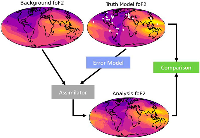
Figure 1. Conceptual diagram for an ionospheric OSSE.

Figure 1 shows a truth model with white dots indicating measurement locations. Measurements are simulated from the truth model, realistic instrumental errors are added to these measurements by the error model, and these measurements are provided to the assimilator, which updates the background for analysis. This analysis is then compared to the truth model to assess the impact of the observation system. OSSET simulates all the data and orchestrates running the assimilator.

2 OSSET data types

The OSSET is designed for ionospheric OSSEs and, therefore, simulates data related to electron density from the truth model. Some of the most common data types are in situ electron density, ionosonde electron density profiles, GNSS total electron content (TEC) from ground stations, and radio occultation (RO) TEC from low earth orbit (LEO) satellites. The OSSET can also simulate TEC from beacon satellites and UV limb and topside soundings, even though these are less common data types. Each of the data types used in this analysis is described below.

2.1 Ionosondes

Ionosondes broadcast HF radiation upward and measure the delay in estimation of the height of the reflecting layer as a function of frequency. The virtual height (h_v) is calculated as h_v = d/(2c), where d is the delay and c is the speed of light in vacuum. Many ionosondes perform the conversion between h_v and the true height h_t by a process called auto-scaling (e.g., Galkin and Reinsch, 2008) and provide both. Auto-scaling is often the largest source of error for ionosondes. The OSSET contains two methods for simulating ionosonde data.

2.1.1 Direct ionosonde simulator

The truth model electron densities are interpolated to the times and location of the ionosonde to make full profiles. Since an ionosonde cannot measure a full profile, measurements that are lower than the highest electron density encountered by an upward moving ray are removed. Next, normally distributed errors with a configurable standard deviation are added to this measurement.

2.1.2 Virtual height ionosonde simulator

A more realistic but more complex way to simulate ionosonde data is to use an HF ray tracer to simulate the delay as a function of frequency and then use an autoscaling software to transform this delay back into the electron density before it is ingested by the assimilator. This process better replicates the main error sources in real ionograms than the direct ionosonde simulator, but it is more computationally expensive. The HF ray tracer used by the OSSET is TRACKER (Argo et al., 1994) and the auto-scaler is POLAN (Titheridge, 1985). This virtual height mode is used in this study instead of the direct method.

2.2 Ground TEC

Ground GPS TEC is simulated by first simulating the satellite positions and filtering for elevation angles above a configurable threshold. Next, a line integral is performed through the truth model electron density to form the TEC. The pseudorange and phase for L1 and L2 are then calculated using the TEC to modify the physical distance between the satellite and the receiver. To add errors, the actual differential code bias for the satellite on that day, elevation-angle-dependent white noise, data gaps, and cycle slips are added. The probability and duration of cycle slips and data gaps are driven by the scintillation indices S4 and σ_ϕ, which are estimated using WBMOD (Secan et al., 1995; Secan and Bussey. 1994).

2.3 Radio occultation TEC

Radio occultation (RO) TEC is a common data type that is available in near real-time from COSMIC-2 (Weiss et al., 2022) as well as commercial vendors (Kursinski et al., 2021; Angling et al., 2021; Chang et al., 2022). In the OSSET, it can be simulated in a prospective or retrospective mode.

2.3.1 Prospective RO simulator

In the prospective mode, the orbit of the LEO satellite is simulated, and the OSSET assumes that if a LEO satellite has a line of sight to a GPS satellite, the TEC is measured. A line integral through the truth model electron density is performed to calculate the TEC, and normally distributed errors with a configurable standard deviation are added. This mode is ideal for optimizing orbital parameters for a future mission.

2.3.2 Retrospective RO simulator

In the retrospective mode, the OSSET uses the files provided by a LEO satellite and replaces the real TEC with TEC computed using a line integral through the truth model. Randomly distributed normal errors with a configurable standard deviation are added. Since this method does not assume that every possible TEC measurement is recorded, it better replicates real-life data dropouts and duty cycles. However, it is not possible for future missions. This is the method used in this study.

3 Comparison of OSE to OSSE

In this section, we compare the OSSET’s predictions of specification improvement to the actual improvement as found through a real-life observation system experiment (OSE). The difference between OSSE prediction and the OSE result is a measure of how well an OSSE will predict real-life performance. For both the OSSE and the OSE, we add commercial RO data to a “baseline” run and measure the increase in accuracy at a group of validation ionosondes. A diagram of this process is shown in Figure 2. For the OSE, the data are divided into two categories: ingest and validation. We assimilate the ingested data and form an analysis. We then compare the analysis to the validation data, which are withheld from the assimilator and are, therefore, independent. For the OSSE, we replicate this exact scenario, except using the truth model instead of taking real measurements.

Figure 2

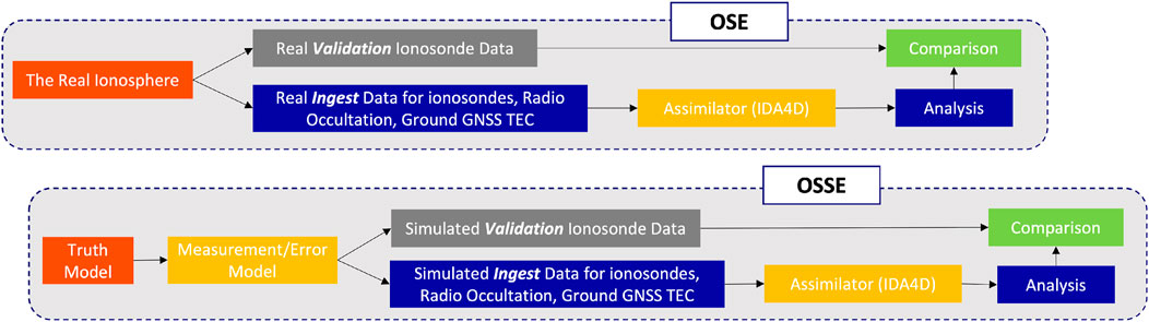
Figure 2. Conceptual diagram for OSSET validation.

This comparison was conducted on 17 Dec 2021, where the planetary K index (K_P) was at or below 2 all day, F10.7 was 117, and the sunspot number was 119, indicating calm geomagnetic and solar conditions. For both the OSSE and OSE, we use the ionospheric data assimilator four-dimensional (IDA4D) model as the assimilator in identical configurations. IDA4D is an assimilator with covariance and state cycling, which accepts a variety of ionospheric data. In addition to the data types used here, it also assimilates UV irradiance and beacon TEC. IDA4D was originally a pure Kalman filter and only accepted data that were linearly related to the state (Bust et al.. 2004). Cycling of the state and covariance and switching from a state of electron density to a state of the logarithm of electron density were added later (Bust et al., 2007; Bust and Datta-Barua, 2014).

Although IDA4D is used in this study, the OSSET has been used with the GPS ionospheric inversion (GPSII) assimilation model (Fridman et al., 2006) as well. We used the international reference ionosphere (IRI, Bilitza et al. (2022)) as a background model. We use a thermosphere–ionosphere–electrodynamics general circulation model (TIE-GCM) (Richmond et al., 1992; Roble et al., 1977) run performed by the community coordinated modeling center (CCMC) as a truth model for its accessibility and reproducibility. This run was performed with TIE-GCM version 2.5 with the Heelis electric field model.

3.1 Data preparation

This study used 26 ionosondes, 36 GNSS ground stations, and all available TEC data from COSMIC-2, as is shown in Figure 3. In Figure 2A, the red squares indicate ionosondes that are not provided to the assimilator and are used for comparison, while the yellow triangles and blue squares are the ingested ground TEC and ionosondes, respectively.

Figure 3

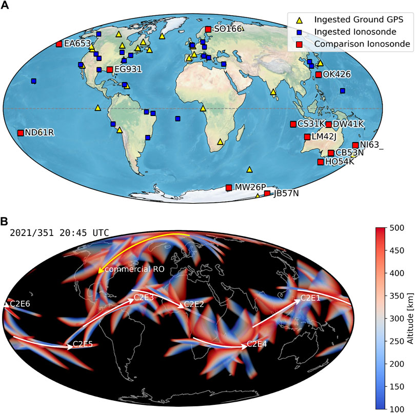
Figure 3. Ingest and validation data for (A) ground and (B) space.

RO data are not as well-localized, which makes it more difficult to visualize. Even for a single measurement, the ray passes through many locations and altitudes on its path from the GNSS satellite to the LEO satellite. As both the satellites move through their orbits and the Earth rotates, the ray paths change as well. The altitude of the ray is shown in color in Figure 2B for a 15-min time window centered on 20:45 UT. Each of the six COSMIC-2 satellite locations is shown as a white line, and the single commercial satellite’s location is shown as a yellow line. This kind of visualization for RO data is referred to as a “fan plot” since the colored wedges showing the ray paths resemble fans. The gaps at the poles from COSMIC-2’s low-inclination orbit are evident in this view.

We use a retrospective mode to simulate the RO data and a prospective mode for the ground GNSS TEC since it is typically of uniform cadence and quite reliable. Although the OSSET does not have a built-in capability to simulate ionosonde data in a retrospective mode, the OSSE ionosonde data are manually truncated to match the OSE data. The ionosonde data are simulated at the minimum OSE cadence (2.5 min), and then any measurement not in the OSE is removed from the OSSE ingest dataset before assimilation to ensure a fair comparison. In addition, we find the minimum frequency in the real ionogram and remove OSSE data below this frequency. This is important since some ionosondes do not measure below 2 or 3 MHz but still provide model-driven data. This better replicates what that actual ionosonde would have measured than assuming a minimum frequency. If this processing is not done, the OSSE can overestimate the real-life improvement dramatically. The counts for each measurement type for the whole 24-h run are shown in Table 1 for each of the four runs. For both the OSE and the OSSE, run 1 ingests the baseline data, and run 2 contains the additional commercial RO data.

Table 1

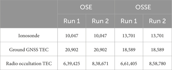
Table 1. Amount of measurements of various types used in each assimilation run.

There are 13 comparison ionosondes and 26 ingested ionosondes. The comparison ionosondes were chosen because they do not provide real-time data and, therefore, are not available for assimilation in a real-time context. Many of these ionosondes happen to be in or near Australia, which slightly affects the statistics. However, using these validation and comparison ionosondes better models a real-life scenario.

Even with the efforts to ensure that the OSSE and OSE have similar quantities of ionosonde data, there are more ingested points in the OSSE than in the OSE. This is because hmF2 was higher in the truth model than in the real ionosphere, which means there are more points for the OSSE. There are also differences in the amount of ingested ground GNSS TEC data. This comes from the error model in the OSSET adding cycle slips and data gaps into the simulated data, which cause some segments of data to be unusable by the assimilator. For this day, the error model over-predicted the amount of data gaps to add, which explains why there are fewer ingested measurements for the OSSE. In contrast to the ground GNSS TEC, there are fewer RO TEC measurements in the OSE than in the OSSE. This is because cycle slips and data gaps are not added in the OSSE error model. In both the OSE and the OSSE, the commercial data adds between 197,375 and 199,246 measurements to run 2, which increases the total amount of RO data by ∼30%. This fractional does not tell the whole story because the commercial data come from a near-polar orbit with more high-latitude coverage.

For both the OSSE and the OSE, it is worth noting that ionosonde data make up approximately 1%–2% of the total data budget, ground GNSS TEC makes up another 2%–3%, and the remaining 95% is made up of RO TEC. There is certainly more ground GNSS TEC available to assimilate—enough to dwarf the RO data—but there is not much more ionosonde data to add. Adding more ground TEC would improve the specification over land masses with a high sensor density, but it would not change dramatically over the oceans.

3.2 Statistical comparison

In all assimilation systems, accuracy increases as more data are added. This section compares this improvement for the OSSE and the OSE. We quantify the improvement in accuracy given in Figure 4. Each of the six subplots shows a 2D histogram comparing a prediction to the validation truth data. The color shows the number of times the combination of the predicted electron density on the y-axis corresponds with the true electron density on the x-axis. A perfect prediction would have all points on the diagonal black dashed line. An inaccurate prediction would have considerable scatter. The mean absolute error (ME) and bias are calculated and shown in the gray box in each sub panel.

Figure 4

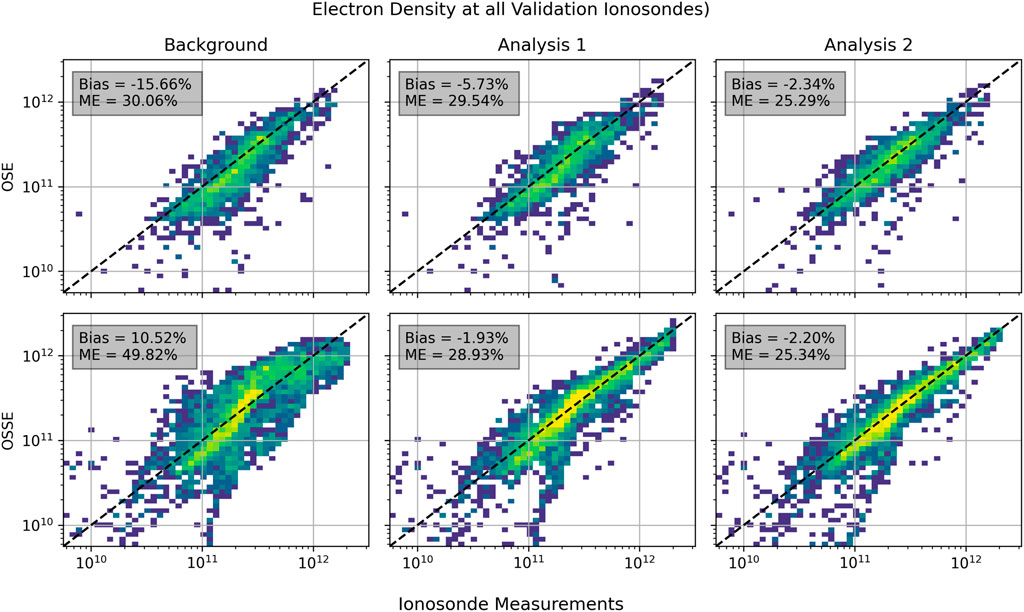
Figure 4. Comparison of OSE and OSSE results. See the text for details.

The top row shows the real OSE, and the bottom row shows the OSSE. In both rows, the leftmost column shows the background (IRI), the middle column shows the first analysis which ingested the baseline data, and the rightmost column shows the second analysis which ingested the baseline data and the additional commercial RO data.

In either row, the scatter becomes visually tighter as one moves from left to right and more data are ingested. The bias and ME parameters also decrease as more data are ingested in all but the OSSE bias, which is already very low in analysis 1. The ability of the OSSE to predict the OSE results is quantified by comparing the bias and ME parameters. This is shown in Table 2, which compiles all the values in the gray boxes in Figure 4.

Table 2

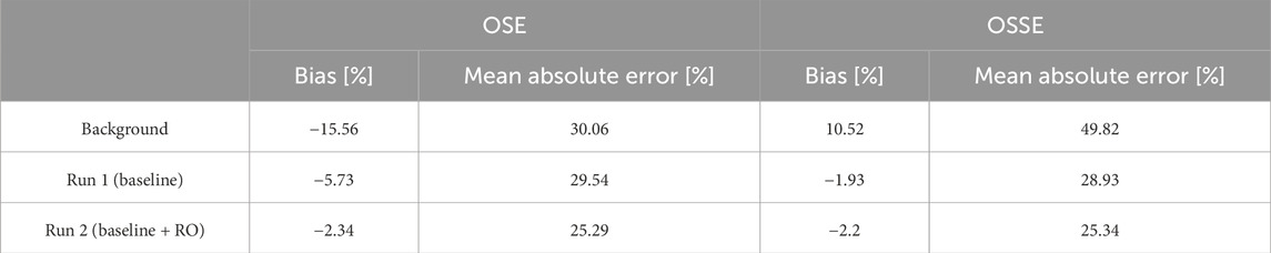
Table 2. Comparison of the bias and mean absolute error for the OSE and OSSE.

The main difference between the OSE and OSSE comparison is the bias. In the OSE, the background electron densities (IRI) are typically ∼15% lower than the real measurements. In the OSSE, the background electron densities are typically ∼10% higher than the comparison measurements simulated with the truth model. This means that the truth model (TIE-GCM) predicts lower electron densities than reality on this day. Although the OSE and OSSE begin with very different background errors, they have similar estimates as to the improvement. Both the OSE and OSSE predict that the baseline data reduce the bias by 8%–10%. However, the MAE improvement differs substantially between the OSSE and the OSE. The OSSE bias gets slightly worse when the commercial RO data are added, likely due to it being driven by the errors added to the measurements rather than the amount of measurements. The OSE and OSSE differ in the ME, with the OSE showing minimal improvement in contrast to the OSSE. However, they both predict a ∼4% decrease when commercial RO data are added.

It is interesting to note that both the bias and ME are nearly identical for the OSE and OSSE in run 2. Given the difference in the amount of ingested data and the single-day comparison, we cannot comment on the generality of this result. Without additional OSE/OSSE comparisons, it is impossible to tell whether the OSSET predicts absolute errors or relative improvements with higher accuracy in general. The differences in the amounts of ingested data shown in Table 1 should also be considered when interpreting these results. The OSSE contains slightly more ionosonde and RO data and slightly less ground GNSS TEC than the OSE.

4 Beyond the OSE

OSEs and OSSEs are complementary; they fill in each other’s gaps. An OSE has the benefit of using all real data and is, therefore, not reliant on the accuracy of the truth model or sensor error model. As shown in Table 2, the OSSET does not perfectly capture the error characteristics of ground and RO TEC. However, an OSE is limited in scope. The OSE shown here can only resolve the improvement in ionospheric specification above the 13 validation ionosondes shown in Figure 2A, which are not evenly distributed over the globe. Additionally, the test data (the commercial RO data in this case) must be taken before an OSE can be performed. OSSEs address many of these limitations—in the prospective mode, the improvement in specification can be assessed before the satellite is even designed. Furthermore, an OSSE can quantify the specification improvement in a place where there is no validation measurement possible. In this OSE, we used ionosonde data, so it is impossible to assess the improvement over the open ocean or above hmF2. Other possible OSE validation datasets have different limitations. For example, an in situ satellite measurement would be globally distributed but would not generally contain measurements below hmF2. Although OSSEs do not have these limitations, they do not use real data and are, therefore, less accurate.

This section demonstrates the unique types of analyses that can be performed with OSSEs that cannot be done with OSEs. We use the improvement of the foF2 specification for this example, but OSSEs can be used to assess many different metrics, such as the increase in the accuracy of coordinate registration for over-the-horizon radars or HF communication availability.

The foF2 results are shown in Figure 5. The left column shows maps of foF2 at 18:45 UT for the truth model; background (IRI); the first analysis, which used the baseline dataset; and the second analysis, which used the baseline and commercial RO data. There are a number of differences between the truth and background models, most striking of which is perhaps the strength of the EIA crest near Hawaii. Both analyses mostly correct this error, which shows the impact of data assimilation. To make the next column, the mean error is computed using Eq. 1:

$E=100\%\times \text{Mean}\left(\frac{x-\text{Truth\hspace{0.17em}foF}2}{\text{Truth\hspace{0.17em}foF}2}\right),(1)$

where x is either the background, analysis 1, or analysis 2 foF2 and the mean is performed across time. This error is shown as color in the second column for the background, analysis 1, and analysis 2. The error near Hawaii is shown very prominently as a red streak. There are also strong negative errors (under predictions of the truth by the background) over much of the continental United States and Asia. There is also an over-prediction near Tierra del Fuego. Note that the background errors are much worse near the North Pole than the South Pole. Many of these error-prone regions are fixed by ingesting data, as shown in the lower number of errors of both analyses. The impact of the data assimilation is quantified by calculating the improvement using Eq. 2:

$I=|E_B|-|E_x|,(2)$

where E_B is the background error (top panel of second column), E_x is the error of either analysis, and |y| indicates the absolute value of y. This variable describes how much each analysis improves relative to the background. It is high (bright yellow) in places where there were initially large errors and enough data to fix them. Note that the improvement in northern Russia and near Tierra del Fuego is stronger in analysis 2 than in analysis 1.

Figure 5

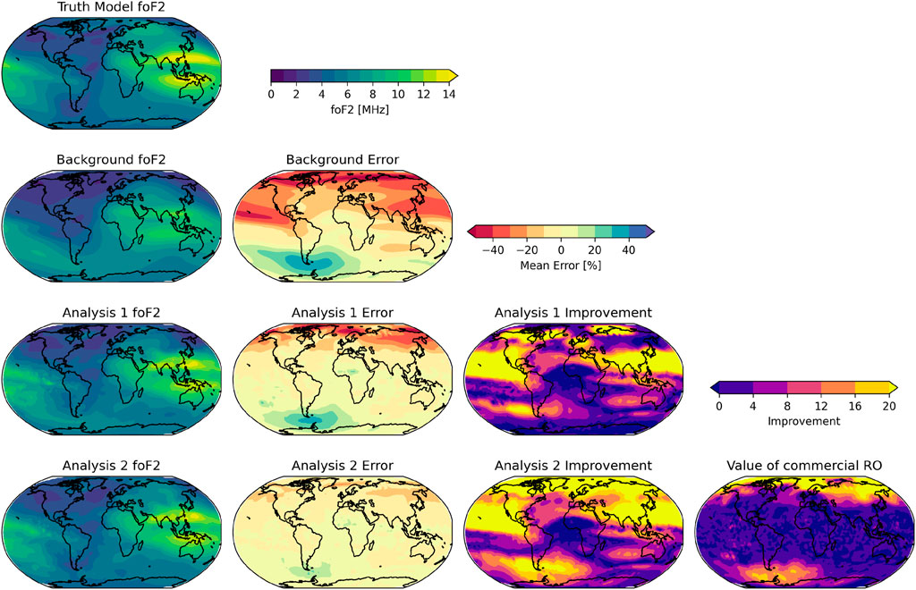
Figure 5. foF2 specification global analysis only possible with an OSSE.

Finally, compute the value of the additional commercial RO data as V = |I_A2| − |I_A1|. This variable captures the increase in accuracy that is due to the additional dataset and is shown in the lower right plot. There are two yellow “halos” near the North and South poles. The reason that the southern halo is not complete is because there are no high errors in the background to resolve at all locations. These high-latitude halos are expected since COSMIC-2 does not provide high-latitude measurements, so there is still room for improvement. At the equatorial and mid-latitude regions, the errors are already mostly resolved by COSMIC-2, so the additional RO data have diminishing returns.

Now we link this value of the additional RO data for specifying foF2 to the increase in the revisit rate. We do this in coordinates of the latitude and local time (LT) instead of the geographic coordinates of latitude and longitude in Figure 6. Local time is a relevant coordinate because the commercial RO satellite is in a sun-synchronous orbit with ascending and descending nodes near 3 and 15 h, respectively. Quantifying the revisit rate for a remote measurement like RO is difficult because the transmitter and receiver both move considerably during an occultation. We divide the ionosphere into voxels of size 2.5° along latitude/longitude and 10 km along altitude and then convert the longitude into local time. For each 10-min chunk of time throughout the day, we compute whether a given voxel was pierced by an RO ray path. The upper left panel of Figure 6 shows the mean visits per hour across the day for just COSMIC-2. Note that there is no coverage at high latitude and that there are no substantial local time trends. The upper right panel shows this metric when the commercial RO data are included. Note the increase in high-latitude coverage and additional coverage near 3 and 15 LT at mid- and low latitudes, respectively. The lower left panel shows the improvement (percent increase in mean visits) that the commercial data yield relative to the baseline of COSMIC-2. In addition to the completely new measurements at high latitudes, there is significant improvement in coverage at mid-latitudes and, for certain local times, at low latitudes. The contour showing latitude/LT bins with 75% or higher increase in revisit rate (dark and light green regions) is computed and shown in white in the lower right panel. In addition to this contour, the value of commercial RO for the foF2 specification is shown in color. The regions of high value descend lower in latitude near 15 LT near the North Pole, which matches the coverage increase contour. This trend is seen to a lesser extent near 3 LT. At the South Pole, the low-latitude improvement is more dramatic near 3 than near 15 LT due to the background error being higher near 0–6 LT than at other times. Analyses such as this are possible only in OSSEs, and they give decision makers more information regarding the impact of any change to their observation system.

Figure 6

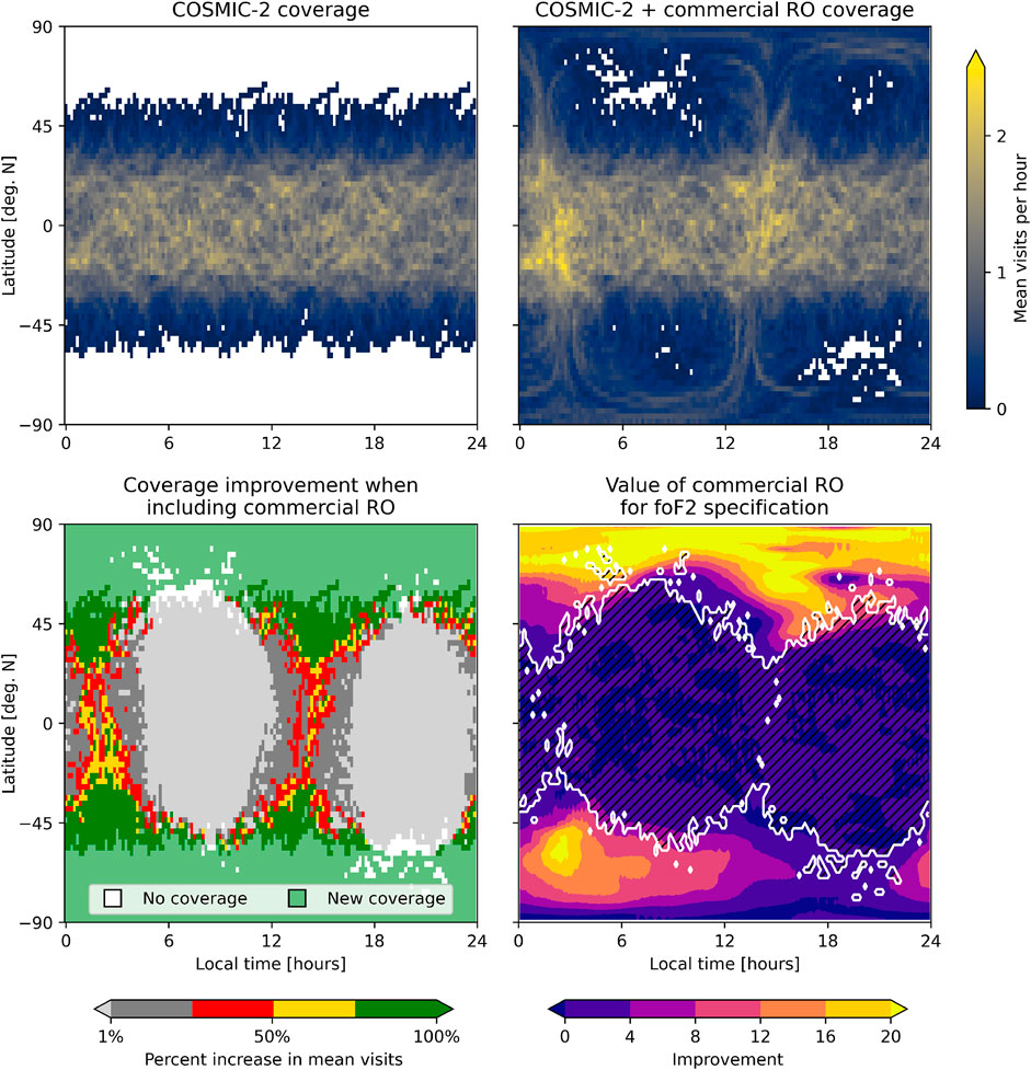
Figure 6. Increase in revisit rate and value of additional RO data for specifying foF2. Upper left: average number of times an RO ray path pierces the ionosphere at the given local time and latitude from 300–310 km in altitude using only COSMIC-2. Upper right: same, but adding the commercial RO data. Lower left: increase in the revisit rate when adding commercial RO. Lower right: Value of commercial RO for specifying foF2 as color, with a white contour showing the boundary where the increase in the revisit rate is higher than 75%.

5 Summary and conclusion

An observation system simulation experiment (OSSE) is a powerful way to understand the sensitivity of an observation system to more data or different configurations. This paper uses the OSSET (the OSSE tool) to perform an OSSE to predict the impact of adding commercial radio occultation data to an electron density specification system. This prediction is carried out in two ways: first, we compare the electron density errors at a group of independent ionosondes before and after adding the data, and second, we compare the global foF2 errors before and after adding the data. For the first assessment, we compare the OSSET’s prediction to that of an OSE using real-life data. Despite different initial biases, the OSE and OSSE predict similar relative improvements in bias and ME. The improvements in global foF2 assessment show preferential improvement of up to 20% at high latitudes, which is to be expected since the baseline data do not include high-latitude RO data.

Although these findings are intuitive and explainable, this study has limitations. We used a single day in winter with moderate solar forcing and quiet geomagnetic conditions. A more robust study would replicate this experiment for different seasons, different points in the solar cycle, and different geomagnetic conditions. Additionally, this study used 13 ionosondes as the comparison dataset and found good agreement between the OSE and the OSSE. From this, we can only speculate as to how well the OSSET would predict a different comparison dataset such as TEC or a HF propagation-related metric. Future work could validate the OSSET for these additional situations and datasets. Future work could also investigate the robustness of the impact of RO data under different conditions.

OSSEs also enable novel analysis that would be impossible in the context of an OSE. We demonstrate this by predicting the global impact of commercial RO data in both geographic and local time coordinates. These both show different aspects of how the errors decrease with additional data. The geographic analysis shows more improvement in the North Pole compared to the South Pole because there are higher errors to begin with. The local time analysis shows that this improvement descends to low latitudes more frequently near 3 and 15 LT, where there are the most additional measurements from the sun-synchronous commercial RO satellites.

Both OSEs and OSSEs have unique and complementary values. OSEs use real data and, therefore, are more trustworthy. However, they have limited value for “what if” questions involving hard-to-measure quantifications or the design of future observation systems. OSSEs do not use real data, and because of this, their predictions are less trustworthy. However, the impact can be assessed in any place and in any way desired.

Data availability statement

Publicly available datasets were analyzed in this study. These data can be found here: https://ccmc.gsfc.nasa.gov/results/viewrun.php?domain=IT&runnumber=Joe_Hughes_031023_IT_1.

Author contributions

JH: data curation, formal analysis, methodology, visualization, writing–original draft, and writing–review and editing. IC: data curation, formal analysis, methodology, visualization, writing–original draft, and writing–review and editing. GC: conceptualization and writing–review and editing. AR: software and writing–review and editing. IA: conceptualization and writing–review and editing.

Funding

The author(s) declare that no financial support was received for the research, authorship, and/or publication of this article.

Acknowledgments

The authors gratefully acknowledge helpful conversations on all things OSSE and OSSET with Victoriya Forsythe, Jeff Steward, Ryan Blay, and Wanli Wu.

Conflict of interest

JL, IC, GC, and AR were employed by the Orion Space Solutions.

The remaining author declares that the research was conducted in the absence of any commercial or financial relationships that could be construed as a potential conflict of interest.

Publisher’s note

All claims expressed in this article are solely those of the authors and do not necessarily represent those of their affiliated organizations, or those of the publisher, the editors, and the reviewers. Any product that may be evaluated in this article, or claim that may be made by its manufacturer, is not guaranteed or endorsed by the publisher.

References

Angling, M. J., Nogués-Correig, O., Nguyen, V., Vetra-Carvalho, S., Bocquet, F.-X., Nordstrom, K., et al. (2021). Sensing the ionosphere with the spire radio occultation constellation. J. Space Weather Space Clim. 11, 56. doi:10.1051/swsc/2021040

CrossRef Full Text | Google Scholar

Argo, P. E., DeLapp, D., Sutherland, C. D., and Farrer, R. G. (1994). Tracker: a three-dimensional raytracing program for ionospheric radio propagation. Tech. rep. Los Alamos, NM, United States: Los Alamos National Lab.

Google Scholar

Bilitza, D., Pezzopane, M., Truhlik, V., Altadill, D., Reinisch, B. W., and Pignalberi, A. (2022). The international reference ionosphere model: a review and description of an ionospheric benchmark. Rev. Geophys. 60. doi:10.1029/2022RG000792

CrossRef Full Text | Google Scholar

Bust, G., Garner, T., and Gaussiran, T. L. (2004). Ionospheric data assimilation three-dimensional (ida3d): a global, multisensor, electron density specification algorithm. J. Geophys. Res. 109. doi:10.1029/2003JA010234

CrossRef Full Text | Google Scholar

Bust, G. S., Crowley, G., Garner, T. W., Gaussiran, T. L., Meggs, R. W., Mitchell, C. N., et al. (2007). Four-dimensional gps imaging of space weather storms. AGU Space Weather 5. doi:10.1029/2006SW000237

CrossRef Full Text | Google Scholar

Bust, G. S., and Datta-Barua, S. (2014). Scientific investigations using IDA4D and EMPIRE (American geophysical union (AGU)). chap. 23.

Google Scholar

Chang, J., Chang, H., and Lee, J. (2022). Cycle slip mitigation for total electron content retrieval using geooptics radio occultation data. Chicago, IL: AGU Fall Meeting.

Google Scholar

Forsythe, V. V., Azeem, I., Blay, R., Crowley, G., Gasperini, F., Hughes, J., et al. (2021). Evaluation of the new background covariance model for the ionospheric data assimilation. Radio Sci. 56, e2021RS007286. doi:10.1029/2021rs007286

CrossRef Full Text | Google Scholar

Fridman, S. V., Nickisch, L. J., Aiello, M., and Hausman, M. (2006). Real-time reconstruction of the three-dimensional ionosphere using data from a network of gps receivers. Radio Sci. 41. doi:10.1029/2005RS003341

CrossRef Full Text | Google Scholar

Galkin, I., and Reinsch, B. (2008). The new artist 5 for all digisondes. Sydney, New South Wales, Austrailia: Ionosonde Network Advisory group Bulletin.

Google Scholar

Hoffman, R., and Atlas, R. (2016). Future observation system simulation experiments. Bull. Am. Meteorological Soc. 97, 1601–1616. doi:10.1175/BAMS-D-15-00200.1

CrossRef Full Text | Google Scholar

Hsu, C. T., Matsuo, T., Yue, X., Fang, T. W., Fuller-Rowell, T., Ide, K., et al. (2018). Assessment of the impact of formosat-7/cosmic-2 gnss ro observations on midlatitude and low-latitude ionosphere specification: observing system simulation experiments using ensemble square root filter. AGU J. Geophys. Res. Space Phys. 123, 2296–2314. doi:10.1002/2017JA025109

CrossRef Full Text | Google Scholar

Kursinski, E., Brandenmeyer, J., Botnik, A., Leidner, M., Leroy, S., and Gooch, R. (2021). Initial validation of planetiq ionosphere measurements via comparisons with cosmic-2 and iri. New Orleans LA: AGU Fall Meeting.

Google Scholar

Pedatella, N. M., Anderson, J. L., Chen, C. H., Raeder, K., Liu, J., Liu, H.-L., et al. (2020). Assimilation of ionosphere observations in the whole atmosphere community climate model with thermosphere-ionosphere extension (waccmx). J. Geophys. Res. Space Phys. 125. doi:10.1029/2020JA028251

CrossRef Full Text | Google Scholar

Richmond, A. D., Ridley, E. C., and Roble, R. G. (1992). A thermosphere/ionosphere general circulation model with coupled electrodynamics. Geophys. Res. Lett. 6, 601–604. doi:10.1029/92gl00401

CrossRef Full Text | Google Scholar

Roble, R. G., Dickinson, R. E., and Ridley, E. C. (1977). Seasonal and solar cycle variations of the zonal mean circulation in the thermosphere. J. Geophys. Res. 82, 5493–5504. doi:10.1029/JA082i035p05493

CrossRef Full Text | Google Scholar

Schreiner, W., Weiss, J., Anthes, R., Braun, J., Chu, V., Fong, J., et al. (2020). Cosmic-2 radio occultation constellation: first results. Geophys. Res. Lett. 47. doi:10.1029/2019GL086841

CrossRef Full Text | Google Scholar

Secan, J. A., and Bussey, R. M. (1994). An improved model of high-latitude F-region scintillation (WBMOD version 13). Tech. rep. NorthWest Research Associates. https://apps.dtic.mil/sti/tr/pdf/ADA288558.pdf.

Google Scholar

Secan, J. A., Bussey, R. M., Fremouw, E. J., and Basu, S. (1995). An improved model of equatorial scintillation. Radio Sci. 30, 607–617. doi:10.1029/94RS03172

CrossRef Full Text | Google Scholar

Titheridge, J. (1985). Ionogram analysis with the generalised program POLAN. tech report. NOAA. https://www.osti.gov/biblio/6068617.

Google Scholar

Weiss, J.-P., Schreiner, W. S., Braun, J. J., Xia-Serafino, W., and Huang, C.-Y. (2022). Cosmic-2 mission summary at three years in orbit. Atmosphere 13, 1409. doi:10.3390/atmos13091409

CrossRef Full Text | Google Scholar

Zeng, X., Atlas, R., Birk, R. J., Carr, F. H., Carrier, M. J., Cucurull, L., et al. (2020). Use of observation system simulation experiments in the United States. Bull. Am. Meteorological Soc. 101, E1427–E1438. doi:10.1175/BAMS-D-19-0155.1

CrossRef Full Text | Google Scholar