 Andreas Shalchi
95% of researchers rate our articles as excellent or good
Learn more about the work of our research integrity team to safeguard the quality of each article we publish.
Find out more
ORIGINAL RESEARCH article
Front. Astron. Space Sci. , 09 May 2024
Sec. Space Physics
Volume 11 - 2024 | https://doi.org/10.3389/fspas.2024.1385820
This article is part of the Research Topic New Insights into High-Energy Processes on the Sun and Their Geospace Consequences View all 10 articles
Introduction: In this article, we revisit the pitch-angle scattering equation describing the propagation of energetic particles through magnetized plasma. In this case, solar energetic particles and cosmic rays interact with magnetohydrodynamic turbulence and experience stochastic changes in the pitch-angle. Since this happens over an extended period of time, a pitch-angle isotropization process occurs, leading to parallel spatial diffusion. This process is described well by the pitch-angle scattering equation. However, the latter equation is difficult to solve analytically even when considering special cases for the scattering coefficient.
Methods: In the past, a so-called subspace approximation was proposed, which has important applications in the theory of perpendicular diffusion. Alternatively, an approach based on the telegraph equation (also known as telegrapher’s equation) has been developed. We show that two-dimensional subspace approximation and the description based on the telegraph equation are equivalent. However, it is also shown that the obtained distribution functions contain artifacts and inaccuracies that cannot be found in the numerical solution to the problem. Therefore, an N-dimensional subspace approximation is proposed corresponding to a semi-analytical/semi-numerical approach. This is a useful alternative compared to standard numerical solvers.
Results and Discussion: Depending on the application, the N-dimensional subspace approximation can be orders of magnitude faster. Furthermore, the method can easily be modified so that it can be used for any pitch-angle scattering equation.
The motion of energetic particles such as cosmic rays through plasma is a complicated stochastic process. It is described via transport equations containing different diffusion parameters. The simplest form of a transport equation which is used in this field is the pitch-angle scattering equation ( Shalchi, 2009; Zank, 2014)
where we have used time t, particle position along the mean magnetic field z, pitch-angle cosine μ, particle speed v, and pitch-angle scattering coefficient Dμμ. The analytical form of the latter parameter is difficult to determine since it contains information about the interaction between magnetohydrodynamic turbulence and energetic and electrically charged particles. Very originally, a quasi-linear approach was developed to determine the coefficient Dμμ (Jokipii 1966). However, this approach is inaccurate, and it fails to describe correctly the scattering of particles at 90° corresponding to μ = 0 (Shalchi 2009). Therefore, the so-called second-order quasi-linear theory (SOQLT) was developed by Shalchi (2005), which provides non-vanishing scattering at μ = 0, resolving the 90°-problem. This theory was further explored analytically in Shalchi et al. (2009), and the so-called isotropic form
was derived in the limit of a stronger turbulent magnetic field. In Eq. 2, the parameter D does not depend on μ, but it is a complicated function of turbulence and particle properties (Shalchi et al., 2009).
In addition to the question of what the correct analytical form of Dμμ is, one desires to find solutions to Eq. 1. However, so far, no exact solution to the pitch-angle scattering equation has been found, and one has to rely on either a numerical approach or approximations. However, one can show that in the late-time limit, the pitch-angle-averaged distribution function
satisfies a diffusion or heat transfer equation of the form
where the parallel spatial diffusion coefficient is related to the pitch-angle scattering coefficient via (Earl, 1974)
The heat transfer equation shown above can easily be solved. For sharp initial conditions, for instance, the solution is simply a normalized Gaussian distribution
centered at z = 0 and having the second moment ⟨z2⟩ = 2κ‖t. One can also write down the more general solution
which depends on the initial distribution M(z′, t = 0) and has a Gaussian integral kernel.
More recently (Tautz and Lerche, 2016 and references therein), it was argued that the diffusive solution does not always provide a good approximation, and one should instead use a telegraph equation of the form
where we have used the telegraph time scale τ. It should be noted that using the telegraph equation instead of the diffusion equation was, in particular, suggested in the context of adiabatic focusing (Litvinenko and Schlickeiser, 2013; Effenberger and Litvinenko, 2014), but this effect is omitted in this paper.
Independently, a two-dimensional subspace approximation to the solution of Eq. 1 has been developed (see Shalchi et al. (2011) for the original description of this approach and Shalchi (2020) for a review). Although this approach provides only an approximation to the solution of Eq. 1 for the isotropic case, it provides a pitch-angle-dependent solution. The two-dimensional subspace approximation was successfully applied in the theory of perpendicular transport and contributed significantly to the development of advanced particle transport theories (Shalchi, 2020; Shalchi, 2021).
In this paper, we revisit pitch-angle scattering and parallel spatial diffusion as well as the corresponding transport equations. Through this study, we aim to perform the following tasks:
1. We review the two-dimensional subspace approximation and summarize the corresponding results.
2. We show the equivalence of the two-dimensional subspace approximation and the telegraph equation.
3. We derive an approximation for the Fourier-transformed distribution function corresponding to the correctly normalized solution of the telegraph equation.
4. We propose an N-dimensional subspace approximation to numerically solve the pitch-angle scattering equation. This approach can be several orders of magnitude faster than standard solvers.
5. All numerical and analytical approaches are compared with each other. This will help us understanding the respective advantages and disadvantages of the different techniques.
Those tasks will be performed in Sections. 2–4, and in Section 5, we provide the summary and and conclusions. This article has several appendices containing mathematical details.
The two-dimensional subspace approximation was originally developed by Shalchi et al. (2011) to solve pitch-angle scattering Equation 1. We summarize the corresponding results, rewrite previously found solutions, and discuss the relation to the telegraph equation as follows. The following three subsections were mostly taken from Shalchi (2020) but have been modified significantly.
For the isotropic scattering coefficient, as given by Eq. 2, the parallel spatial diffusion coefficient is obtained via Eq. 5. Alternatively, we can compute the parallel mean free path that is defined via λ‖ = 3κ‖/v. For the isotropic case, those parameters are given by
Eq. 1 corresponds to a partial differential equation with the variables t, z, and μ. As a first step toward a solution, we use the Fourier transform
so that the pitch-angle scattering equation becomes
The inverse Fourier transform is then given by the following equation:
For the isotropic scattering coefficient, Eq. 11 is simplified to
To continue, we expand the solution of Eq. 13 in a series of Legendre polynomials
where the coefficients Cn are functions of time, though they also depend on k. This dependence is not explicitly written down during the following investigations. Using Eq. 14 in the differential Equation 13 yields
where
and
With those two relations, Eq. 15 can be written as follows:
To continue, we multiply this equation by the Legendre polynomial Pm, integrate over μ, and use the orthogonality relation of Legendre polynomials (Abramowitz and Stegun, 1974)
After performing those steps, we derive the recurrence relation
Alternatively, one can use the coefficient Qm defined via
With this, the recurrence relation can be written as follows
For the case of no scattering D = 0, we can compare this with the relation (see Equation of Abramowitz and Stegun (1974))
where we have used spherical Bessel functions. Thus, we find Qm = jm(vkt) for the scatter-free case and
Using this in Eq. 14 yields
where we have used Equation 92 from Shalchi et al. (2011). This is also known as plane wave expansion widely used in quantum mechanics. It should be noted that Eq. 25 corresponds to the unperturbed or scatter-free solution. It can be easily obtained directly from Eq. 11 for the case D = 0.
We use Eq. 20 which corresponds to an infinite set of coupled ordinary differential equations. For m = 0, for instance, we find
and for m = 1, we obtain
It is problematic here that the coefficients C0 and C1 are coupled to C2. Therefore, it is not possible to derive an exact solution for the coefficients Cn.
Since an exact solution to Eq. 20 seems impossible to be found, one needs to rely on approximations. In the following, we discuss the two-dimensional (2D) subspace approximation originally developed by Shalchi et al. (2011), meaning we set
so that only the coefficients C0 and C1 are used. In Lasuik and Shalchi (2019), one can find the solution obtained by using a three-dimensional subspace approximation. It is shown that the three-dimensional (3D) solution is too complicated for most applications.
Within the two-dimensional subspace approximation, the expansion (14) is reduced to
In this case, Eqs 26, 27 can be combined to eliminate C1. Since we set C2 = 0, we found the second-order differential equation
Using the ansatz
leads to the quadratic equation
Alternatively, for C2 = 0, Eqs 26, 27 can be written as the matrix equation
After using Eq. 31 for both functions C0(t) and C1(t), the problem of finding the two ω is expressed as
leading to the same quadratic equation as given by Eq. 32. The latter equation can easily be solved by the following equation:
We conclude that the eigenvalues can be complex depending on the wave number k. With this, the coefficient C0 can be written as the linear combination
with the two unknown coefficients b±. It follows from Eq. 26 that
The coefficients b± will be determined below. Before we perform this task, we write down the solution for Fk(μ, t). We need to combine Eq. 29 with Eqs 36, 37 to derive
In order to find the coefficients b±, we can use the initial condition
meaning that the particle has its initial position at z = 0 and the initial pitch-angle cosine μ0. Using this in the inverse Fourier transform given by Eq. 12, yields after some straightforward algebra
The latter initial condition used in expansion (Eq. 14) allows us to write
In order to determine the coefficients Cn(t = 0), we multiply this by Pm and integrate over μ to get
To perform this task, we have used again the orthogonality relation (Eq. 19). For m = 0 and m = 1, this yields1
and
To determine the coefficients b±, we write down Eqs 36, 37 for t = 0 and use Eqs 43, 44 to deduce
This system of two equations is solved by the following equation
Using this result and Eq. 35 in Eq. 38 provides the two-dimensional subspace approximation to the solution Fk(μ, t). In Section 2.4, we provide a more detailed discussion of this solution.
Our solution is based on the expansion given by Eq. (29). One can easily demonstrate using Eq. 3 and
together with the orthogonality relation (Eq. 19), that the function C0(t) corresponds to the Fourier transform of the pitch-angle-averaged distribution function M(z, t), and C1(t) corresponds to the Fourier transform of the current density or diffusion flux J(z, t). Those two quantities are related to each other via the one-dimensional continuity equation
which is obtained by averaging Eq. 1 over all μ and using Eqs 3, 47. The exact relations to the coefficients are
and
It should be noted that the latter relation is obtained by combining Eq. 47 with Eq. 10 and the expansion given by Eq. 14. After combining these three relations and using the orthogonality relation (Eq. 19), one can obtain Eq. 50. As demonstrated, the coefficients C0(t) and C1(t) are directly linked to physical quantities. In particular, the coefficient C0(t) is very important because it is simply the Fourier transform of the pitch-angle-averaged distribution function M(z, t).
An important quantity in particle transport theory is the characteristic function ⟨e±ikz⟩. We define the ensemble average via
It should be noted that in some cases, one could aim for a result that depends on μ0. Then, the corresponding average is omitted.
To determine the characteristic function, we average over all quantities, and thus, we have
Replacing f(z, μ, t) therein by using Eq. 12 leads to
We now replace Fk(μ, t) by using Eq. 14 and use P0(μ) = 1 to get
Due to the orthogonality of Legendre polynomials (Eq. 19), this is reduced to
To solve the remaining integral, we use Eq. 36 to write
In order to replace b±, we use Eq. 46. The integrals over the terms containing μ0 vanish, and we finally find
It should be noted that the parameters ω± are given by Eq. 35. For the case that the ω± are real, the characteristic function given by Eq. 57 is real as well. For the case that the ω± are complex, it follows from Eq. 35 that
Based on Eq. 35, it can be shown that Eq. 57 contains two asymptotic limits, namely, (see Shalchi (2020) for more details)
For small wave numbers, we find the characteristic function of diffusion Equation 4. The result obtained for large wave numbers can be understood as a damped unperturbed orbit.
By comparing Eq. 53 with Eq. 10 and using Eq. 3, we can relate the characteristic function to the μ- and μ0-averaged functions M(z, t). This relation is given by the following equation:
Furthermore, we can compare this with Eq. 49 to find
As an example, we consider the limit D → ∞ so that we can use the first line of Eq. 58 in Eq. 59. We can easily derive
corresponding to a Gaussian solution. The result obtained here is the diffusive solution that one would expect in this case (see Eq. 6 in this paper).
Other physical quantities can be derived by using the subspace approximation, alternative approximations, or even exact calculations (Shalchi, 2006; Shalchi, 2011).
Eq. 29 corresponds to an integral representation of the solution of the Fourier-transformed pitch-angle scattering equation. This result is based on the 2D subspace approximation. Using therein Eqs 36 and 37, as well as (Eq. 46) yields
where the functions ω± are given by Eq. 35.
The μ- and μ0-averaged solution is then
in Fourier space. To find the solution in the configuration space, we use Eq. 10 to derive
Alternatively, this result can also be obtained by combining Eqs 57, 59.
It is convenient to define the parameter
and it follows from Eq. 35 that
From this, we can easily deduce
Therewith, the solution in the configuration space is given as the following Fourier transform
where we have used the integrand, which is an even function of k. With the help of hyperbolic functions, this can be written in a more compact form
It should be noted that the quantity ξ, given by Eq. 65, can either be real or imaginary depending on the value of k. Eq. 69 provides an integral representation of the μ- and μ0-averaged distribution function based on the 2D subspace approximation. Alternative forms are presented in Supplementary Appendix S1 of this paper. In Supplementary Appendix S2, we provide an approximative solution of the remaining integral.
We have derived an ordinary differential equation for the function C0(t) previously (Eq. 30), which can be written as follows
As shown via Eq. 49, C0(t) is the Fourier transform of the distribution function M(z, t). Thus, working in the configuration space instead of the Fourier space allows us to write Eq. 70 as
The latter equation has the same form as Eq. 8, and, thus, it corresponds to a telegraph equation. A quick alternative derivation of the latter equation can be found in Supplementary Appendix S3. It should be noted that the coefficient C0(t) used here depends also on the initial pitch-angle cosine μ0. If one averages over the latter quantity, the two-dimensional subspace approximation provides Eq. 69. In Supplementary Appendix S4, we demonstrate that the latter form indeed solves Eq. 71. Using therein Eq. 9 and the scattering time τ = 1/(2D) yields the telegraph equation, as given by Eq. 8. Therefore, we have shown the complete equivalence of the two-dimensional subspace approximation and the telegraph equation. The solution given by Eq. 69 is correctly normalized. In order to demonstrate this, we consider
Therein, we use (Zwillinger, 2012)
to write this as
From Eq. 65, it follows that ξk=0 = D, and, thus, we find
As already pointed out in Tautz and Lerche (2016), one can use the transformation
and Eq. 8 becomes
This corresponds to the Klein–Gordon equation but with imaginary mass. After comparing Eqs 69, 76 with each other, we can easily read off the function
We have focused on the function C0(t) previously. We can also derive an ordinary differential equation for C1(t). By combining Eqs 26, 27, we derive
where we have set C2 = 0 corresponding to the 2D subspace approximation. Eq. 78 is the same equation as we have derived above for C0. The function C1(t) corresponds to the Fourier-transformed current density, as shown by Eq. 50. Therefore, the telegraph and Klein–Gordon equations can also be derived for the current density function. In order to obtain the current density, as a further solution to the telegraph equation, we can combine Eq. 69 with the continuity Equation 48. We can easily derive
where ξ is given by Eq. 65. Of course, integrating the obtained
Previously, we have used the expansion in the Legendre polynomials (see Eq. 14 of this paper). The functions Cn(t) therein are given by the recurrence relation (Eq. 20). This relation is still exact and can be written as the following matrix equation
with the tridiagonal matrix A having the components
The vector
where we have used the matrix exponential. The initial conditions Cn(t = 0) are given by Eq. 42. Eq. 82 can be easily evaluated with software such as MATLAB. However, it is required to work with a finite matrix A. This corresponds to the subspace approximation outlined above. Let us assume that we work with an N × N-matrix. This then corresponds to an N-dimensional subspace approximation. The method described here corresponds to a semi-numerical/semi-analytical approach that solves the pitch-angle scattering equation, but this method can be faster if one needs the solution only for a specific time t. Standard numerical solvers (see Supplementary Appendix S5 of this paper) require a high time resolution to be accurate. Therefore, one typically needs to work with roughly thousand time-steps so that the solution converges to the true solution of the differential equation. The N-dimensional subspace approximation can be applied to a single time value. As shown via Figures 2–9, an accurate solution is obtained for N = 10.
For certain applications, one could be interested in the μ- and μ0-averaged solution only. Analytical solutions of diffusion and telegraph equations are incomplete and inaccurate depending on the considered application. For the case of pitch-angle-averaged solutions, the N-dimensional subspace approximation is particularly powerful, as outlined below. First, we define the matrix exponential used already above via
Then, Eq. 82 can be written as follows
or in component notation,
At the initial time, the components of the vector
meaning that all coefficients are 0, except C0(t = 0). Therefore, we can write the time-dependent coefficients as
Furthermore, the μ-dependent solution is given by Eq. 14. After μ-averaging of the latter expansion, we find
where Mk(t) is the Fourier-transformed distribution function as observed by Eq. 49. It should be noted that the function C0(t) discussed here is also μ0-averaged. Furthermore, the characteristic function is easily obtained via
meaning that the 00-component is simply the characteristic function. Thus, it follows from Eq. 59 that
which is an integral and matrix exponential representation of the μ- and μ0-averaged distribution function. Therefore, in order to obtain the distribution function M(z, t) for given z and t, we need to numerically solve the k-integral in Eq. 90. For each value of k, we set up the matrix A defined via Eq. 81, numerically compute the matrix exponential E, and use the component E00 in the numerically evaluated k-integral. The distribution functions shown in Figures 6, 7, based on the 10D subspace approximation, for instance, can be computed with a regular computer within a few seconds. Figure 1 shows a comparison in speed between different numerical methods. This comparison includes the N-dimensional subspace approximation described above and the pure numerical approach described in Supplementary Appendix S5 of this paper, which corresponds to an implicit Euler method.
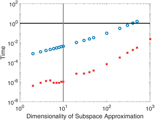
Figure 1. Shown are runtimes of codes used to solve the pitch-angle scattering equation based on different techniques. The black horizontal line represents the pure numerical solution, providing a result which depends on the pitch-angle cosine μ and the initial pitch-angle cosine μ0. This pure numerical method is described in Supplementary Appendix S5 and corresponds to an implicit Euler method. The blue circles represent the N-dimensional subspace approximation described in Section 3 also providing a pitch-angle-dependent result. The red crosses represent the N-dimensional subspace approximation for the μ- and μ0-averaged case. For a small dimensionality (small N), the runtimes are insignificant. It should also be noted that one obtains an accurate result for N = 10 (vertical gray line), meaning that the subspace approximation is several orders of magnitude faster than standard numerical solvers. It should be noted that all results are normalized with respect to the runtime of the pure numerical method and have been obtained by using MATLAB running on the same computer.
The μ- and μ0-dependent Fourier-transformed solution is given by the following equation:
where we have combined Eqs 14, 42, and 85. The Fourier transform can be performed using Eq. 10 and solving the k-integral numerically. Of course, obtaining and plotting the pitch-angle-dependent result is more time-consuming when compared to the pitch-angle-averaged solution.
In certain analytical theories developed for describing the perpendicular transport of energetic particles, one needs to know the function (Shalchi, 2010; Shalchi, 2017; Shalchi, 2020; Shalchi, 2021)
that is somewhat similar but not identical compared to the characteristic function discussed above. In order to express Γk(t) as before, we perform the same mathematical steps. The pitch-angle-dependent solution is given by Eq. 14. In order to obtain Γk(t), we need
To evaluate this further, we use Eqs 12, 14. After using those two relations, we derive
For the μ-integral, we can use the orthogonality relation (Eq. 19) to find
Using the above relation allows us to perform the following steps:
where we have used Eqs 19, 42, and 85. Therefore, the derived function
We have solved the pitch-angle scattering equation numerically using an implicit Euler method (Supplementary Appendix S5) and the N-dimensional subspace approximation outlined in the previous section. We have considered two cases, namely, N = 2 (corresponding to the pure analytical case discussed above) and N = 10 (which provides an accurate result). In most cases, we have only considered the μ-averaged solution to reduce the number of plots. Some results are also averaged over the initial pitch-angle cosine μ0.
Figures 2–5 show the characteristic function ⟨eikz⟩≡⟨e−ikz⟩, which corresponds to the Fourier transform of the distribution function
Figures 4, 5 show the characteristic function versus time
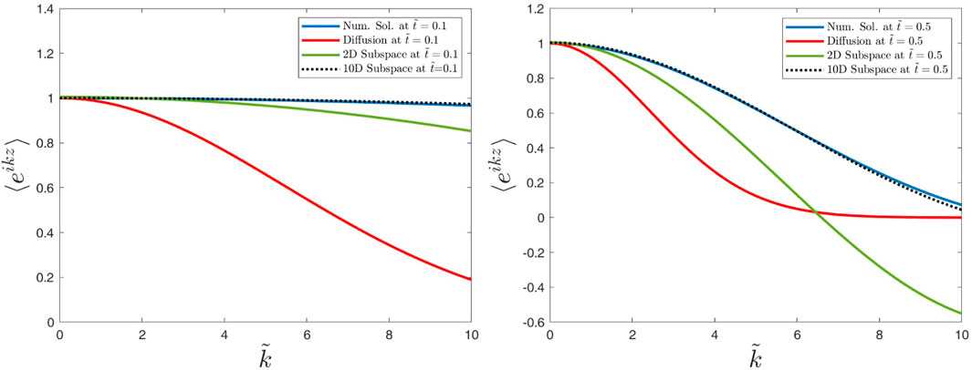
Figure 2. Numerical and analytical solutions obtained for the characteristic function ⟨eikz⟩ versus the dimensionless wave number
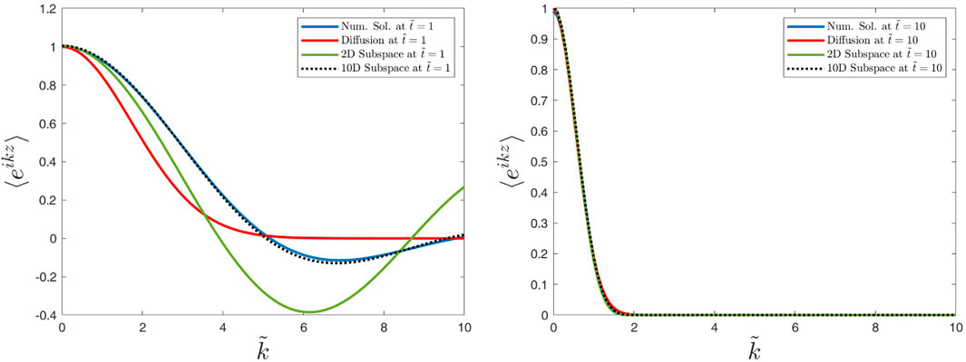
Figure 3. Caption is as in Figure 2, but we have considered the times
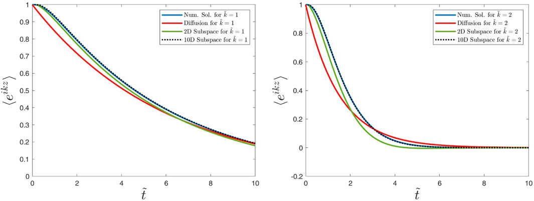
Figure 4. Numerical and analytical solutions obtained for the characteristic function ⟨eikz⟩ versus dimensionless time
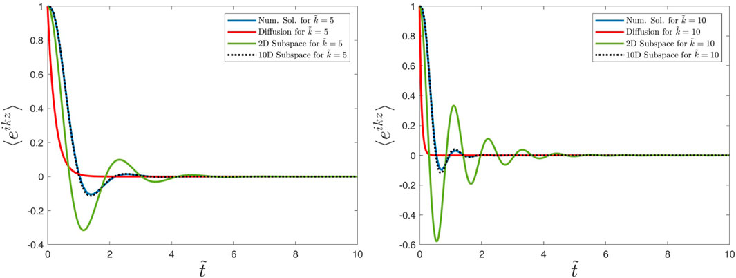
Figure 5. Caption is as in Figure 4, but we have considered the values
Figures 6–9 show the distribution function
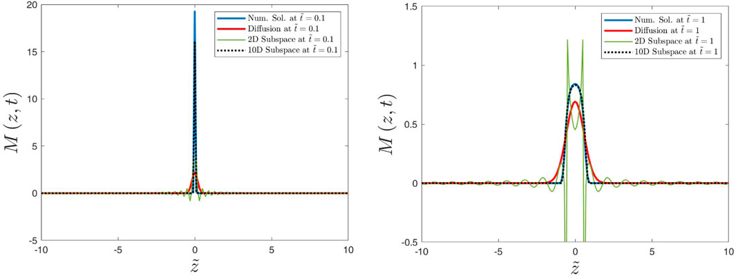
Figure 6. Numerical and analytical solutions for the μ-averaged distribution function M(z, t) versus the parallel position
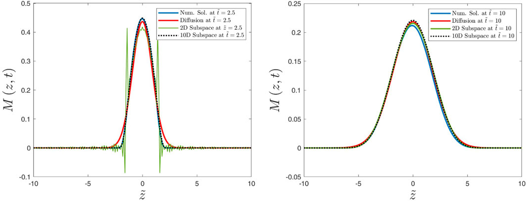
Figure 7. Caption is as in Figure 6, but we have considered the times
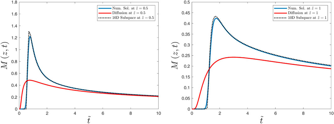
Figure 8. Numerical and analytical solutions for the μ-averaged distribution function M(z, t) versus time
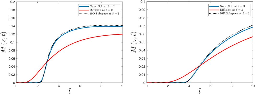
Figure 9. Caption is as in Figure 8, but we have considered
Figure 10 shows the comparison of the time evolution of
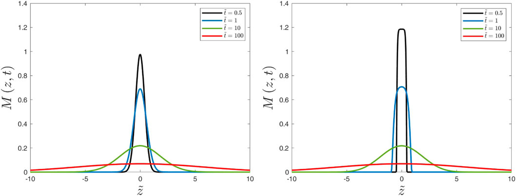
Figure 10. Time evolution of distribution functions. The left panel shows the solution of the diffusion equation as given by Eq. 6 for different times, and the right panel shows the μ0-and μ-averaged solutions of the pitch-angle scattering equation based on the 10D dimensional subspace approximation.
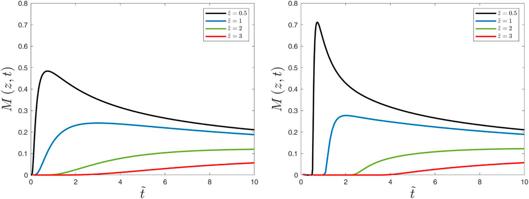
Figure 11. Distribution functions versus time
Last but not the least, we have computed the function
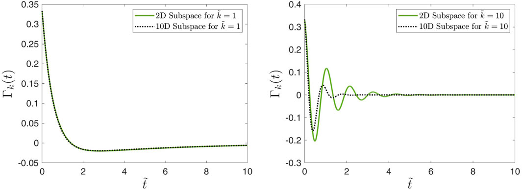
Figure 12. Numerical results for the function Γk(t) as defined via Eq. 92 based on 2D and 10D subspace approximations. The left panel shows results for
In this paper, we have focused on the most basic transport equation, namely, the pitch-angle scattering equation, as given by Eq. 1. Analytical and numerical investigations of pitch-angle-dependent transport equations have been the subject of several papers published during recent years. In addition to studies of the basic pitch-angle scattering equation (Shalchi et al., 2011; Tautz and Lerche, 2016; Lasuik and Shalchi, 2017; Lasuik and Shalchi, 2019), authors have explored the impact of so-called focusing, an effect which is related to a non-constant mean magnetic field (Danos et al., 2013; Litvinenko and Schlickeiser, 2013; Effenberger and Litvinenko, 2014; Lasuik et al., 2017; Wang and Qin, 2020; Wang and Qin, 2021; Wang and Qin, 2023). Even more complicated cases, including perpendicular particle transport, have been investigated by Wang and Qin (2024).
In this article, we have reviewed the two-dimensional subspace approximation originally developed by Shalchi et al. (2011) and discussed the provided solutions in configuration and Fourier spaces. We have also demonstrated that the two-dimensional subspace approximation is equivalent to using a telegraph equation. Normalized solutions in configuration and Fourier spaces are also discussed. However, we also argue that such solutions do not often provide appropriate results even if the pitch-angle average is considered. Although it was often argued that the telegraph equation is more complete than the usual diffusion approach (Tautz and Lerche, 2016), the solution discussed here contains artifacts that are not realistic. In particular, we observe spikes at z = ±vt (Figures 6, 7 as well as Supplementary Appendix S2).
Therefore, it is important to solve the pitch-angle scattering equation numerically. However, standard approaches such as implicit Euler or Crank–Nicolson solvers are time-consuming to use. In this paper, we have, thus, developed an N-dimensional subspace approach. This method can be seen as a semi-analytical/semi-numerical method. It has the advantage of being is several orders of magnitude faster than standard solvers (see Figure 1 of this paper). This is in particular the case if one is only interested in pitch-angle-averaged solutions at a given time. Standard solvers require a high time resolution in order to provide an accurate result. The N-dimensional subspace technique can be applied for a single time value if this is everything what is needed. It should also be emphasized that the N-dimensional subspace method can be easily parallelized since for a given k and t, one can compute the matrix exponentials independently of other values. This is also valid if one is looking for a μ- and μ0-dependent result.
In this paper, we have computed several quantities such as distribution and characteristic functions as well as the function
It has to be noted that the N-dimensional subspace method presented in this paper was specifically developed for the basic pitch-angle scattering equation and an isotropic scattering coefficient. However, this approach can be easily modified so that it can be used for more general transport equations including focused transport equations and other forms of the pitch-angle scattering coefficient.
The original contributions presented in the study are included in the article/Supplementary Material; further inquiries can be directed to the corresponding author.
AS: writing–original draft and writing–review and editing.
The author(s) declare that financial support was received for the research, authorship, and/or publication of this article. The authors also acknowledge the support by the Natural Sciences and Engineering Research Council (NSERC) of Canada.
The author declares that the research was conducted in the absence of any commercial or financial relationships that could be construed as a potential conflict of interest.
All claims expressed in this article are solely those of the authors and do not necessarily represent those of their affiliated organizations, or those of the publisher, the editors, and the reviewers. Any product that may be evaluated in this article, or claim that may be made by its manufacturer, is not guaranteed or endorsed by the publisher.
The Supplementary Material for this article can be found online at: https://www.frontiersin.org/articles/10.3389/fspas.2024.1385820/full#supplementary-material
1Note: there is a typo in Shalchi (2020) where one can find the incorrect formula C0(t = 0) = 1/(3π).
Abramowitz, M., and Stegun, I. A. (1974). Handbook of mathematical functions. New York: Dover Publications.
Crank, J., and Nicolson, P. (1947). A practical method for numerical evaluation of solutions of partial differential equations of the heat conduction type. Proc. Camb. Phil. Soc. 43, 50–67. doi:10.1017/s0305004100023197
Danos, R. J., Fiege, J. D., and Shalchi, A. (2013). Numerical analysis of the fokker-planck equation with adiabatic focusing: isotropic pitch-angle scattering. Astrophysical J. 772, 35. doi:10.1088/0004-637x/772/1/35
Earl, J. A. (1974). The diffusive idealization of charged-particle transport in random magnetic fields. Astrophys. J. 193, 231. doi:10.1086/153152
Effenberger, F., and Litvinenko, Y. E. (2014). The diffusion approximation versus the telegraph equation for modeling solar energetic particle transport with adiabatic focusing, I. Isotropic pitch-angle scattering. Astrophysical J. 783, 15. doi:10.1088/0004-637x/783/1/15
Gradshteyn, I. S., and Ryzhik, I. M. (2000). Table of integrals, series, and products. New York: Academic Press.
Jokipii, J. R. (1966). Cosmic-Ray propagation. I. Charged particles in a random magnetic field. Astrophys. J. 146, 480. doi:10.1086/148912
Lasuik, J., Fiege, J. D., and Shalchi, A. (2017). Numerical analysis of the Fokker-Planck equation with adiabatic focusing: realistic pitch-angle scattering. Adv. Space Res. 59, 722–735. doi:10.1016/j.asr.2016.10.027
Lasuik, J., and Shalchi, A. (2017). Solutions of the cosmic ray velocity diffusion equation. Adv. Space Res. 60, 1532–1546. doi:10.1016/j.asr.2017.06.035
Lasuik, J., and Shalchi, A. (2019). Subspace approximations to the cosmic ray Fokker-Planck equation. Mon. Notices R. Astronomical Soc. 485, 1635–1650. doi:10.1093/mnras/stz474
Litvinenko, Y. E., and Schlickeiser, R. (2013). The telegraph equation for cosmic-ray transport with weak adiabatic focusing. A A 554, A59. doi:10.1051/0004-6361/201321327
Press, W. H., Teukolsky, S. A., Vetterling, W. T., and Flannery, B. P. (2007). Numerical Recipes. Cambridge University Press.
Shalchi, A. (2005). Second-order quasilinear theory of cosmic ray transport. Phys. Plasmas 12, 052905. doi:10.1063/1.1895805
Shalchi, A. (2006). Analytical investigation of the two-dimensional cosmic ray Fokker-Planck equation. Astronomy Astrophysics 448, 809–816. doi:10.1051/0004-6361:20053664
Shalchi, A. (2009). Nonlinear cosmic ray diffusion theories. Astrophysics Space Sci. Libr. 362. Springer, Berlin. doi:10.1007/978-3-642-00309-7
Shalchi, A. (2010). A unified particle diffusion theory for cross-field scattering: subdiffusion, recovery of diffusion, and diffusion in 3D turbulence. Astrophys. J. 720, L127–L130. doi:10.1088/2041-8205/720/2/l127
Shalchi, A. (2011). Velocity correlation functions of charged particles derived from the fokker-planck equation. Adv. Space Res. 47, 1147–1164. doi:10.1016/j.asr.2010.12.002
Shalchi, A. (2017). Time-dependent perpendicular transport of energetic particles in magnetic turbulence with transverse complexity. Phys. Plasmas 24, 050702. doi:10.1063/1.4982805
Shalchi, A. (2020). Perpendicular transport of energetic particles in magnetic turbulence. Space Sci. Rev. 216, 23. doi:10.1007/s11214-020-0644-4
Shalchi, A. (2021). Perpendicular diffusion of energetic particles: a complete analytical theory. Astrophys. J. 923, 209. doi:10.3847/1538-4357/ac2363
Shalchi, A., Škoda, T., Tautz, R. C., and Schlickeiser, R. (2009). Analytical description of nonlinear cosmic ray scattering: isotropic and quasilinear regimes of pitch-angle diffusion. Astron. Astrophys. 507, 589–597. doi:10.1051/0004-6361/200912755
Shalchi, A., Tautz, R. C., and Rempel, T. J. (2011). Test-particle transport: higher-order correlations and time-dependent diffusion. Plasma Phys. control. Fusion 53, 105016. doi:10.1088/0741-3335/53/10/105016
Tautz, R. C., and Lerche, I. (2016). Application of the three-dimensional telegraph equation to cosmic-ray transport. Res. Astronomy Astrophysics 16, 162. doi:10.1088/1674-4527/16/10/162
Wang, J. F., and Qin, G. (2020). The invariance of the diffusion coefficient with iterative operations of the charged particle transport equation. Astrophysical J. 899, 39. doi:10.3847/1538-4357/aba3c8
Wang, J. F., and Qin, G. (2021). Study of momentum diffusion with the effect of adiabatic focusing. Astrophysical J. Suppl. Ser. 257, 44. doi:10.3847/1538-4365/ac1bb3
Wang, J. F., and Qin, G. (2023). Relationship of transport coefficients with statistical quantities of charged particles. Astrophysical J. 954, 213. doi:10.3847/1538-4357/ace9d3
Wang, J. F., and Qin, G. (2024). The effect of solar wind on charged particles’ diffusion coefficients. Astrophysical J. 961, 6. doi:10.3847/1538-4357/ad09b7
Watson, G. N. (2011). A treatise on the theory of Bessel functions. Cambridge: Cambridge Mathematical Library.
Zank, G. P. (2014). Transport processes in space Physics and astrophysics. Lect. Notes Phys. 877. Springer, New York. doi:10.1007/978-1-4614-8480-6
Keywords: cosmic rays, magnetic fields, turbulence, diffusion, transport
Citation: Shalchi A (2024) Transport of energetic particles in turbulent space plasmas: pitch-angle scattering, telegraph, and diffusion equations. Front. Astron. Space Sci. 11:1385820. doi: 10.3389/fspas.2024.1385820
Received: 13 February 2024; Accepted: 05 April 2024;
Published: 09 May 2024.
Edited by:
Gang Li, University of Alabama in Huntsville, United StatesReviewed by:
Patricio A. Muñoz, Technical University of Berlin, GermanyCopyright © 2024 Shalchi. This is an open-access article distributed under the terms of the Creative Commons Attribution License (CC BY). The use, distribution or reproduction in other forums is permitted, provided the original author(s) and the copyright owner(s) are credited and that the original publication in this journal is cited, in accordance with accepted academic practice. No use, distribution or reproduction is permitted which does not comply with these terms.
*Correspondence: Andreas Shalchi, YW5kcmVhc200QHlhaG9vLmNvbQ==
Disclaimer: All claims expressed in this article are solely those of the authors and do not necessarily represent those of their affiliated organizations, or those of the publisher, the editors and the reviewers. Any product that may be evaluated in this article or claim that may be made by its manufacturer is not guaranteed or endorsed by the publisher.
Research integrity at Frontiers
Learn more about the work of our research integrity team to safeguard the quality of each article we publish.