Observation of vertical coupling during a major sudden stratospheric warming by ICON and GOLD: a case study of the 2020/2021 warming event

The response of the thermospheric daytime longitudinally averaged zonal and meridional winds and neutral temperature to the 2020/2021 major sudden stratospheric warming (SSW) is studied at low-to middle latitudes (0^◦ - 40^◦N) using observations by NASA’s ICON and GOLD satellites. The major SSW commenced on 1 January 2021 and lasted for several days. Results are compared with the non-SSW winter of 2019/2020 and pre-SSW period of December 2020. Major changes in winds and temperature are observed during the SSW. The northward and westward winds are enhanced in the thermosphere especially above ∼140 km during the warming event, while temperature around 150 km drops up to 50 K compared to the pre-SSW phase. Changes in the zonal and meridional winds are likely caused by the SSW-induced changes in the propagation and dissipation conditions of internal atmospheric waves. Changes in the horizontal circulation during the SSW can generate upwelling at low-latitudes, which can contribute to the adiabatic cooling of the low-latitude thermosphere. The observed changes during the major SSW are a manifestation of long-range vertical coupling in the atmosphere.

1 Introduction

Sudden stratospheric warmings (SSWs) are remarkable thermodynamical phenomena that occur in the polar lower stratosphere (mostly in the Northern Hemisphere) during winters and last for several days. There are five types of warming events identified as major, midwinter, minor, final, and Canadian (Butler et al., 2015). However, they are often categorized as either major or minor warming events, which are clearly distinguished from each other by the variation of the stratospheric zonal mean zonal winds $\bar{u}$. In a major warming, the zonal mean winds at 60^◦N reverse their direction from eastward to westward at or below 10 hPa (∼30 km) and the zonal mean temperature $\bar{T}$ increases poleward of 60^◦N, meaning that the equator-to-pole temperature gradient reverses its direction. During a minor warming, the zonal mean temperature increases poleward of 60^◦N, while the eastward zonal mean winds weaken but do not fully reverse. SSWs are caused by the large-scale planetary waves propagating upward from the troposphere and interacting with the stratospheric mean flow via dissipation (Matsuno, 1971; Holton, 1976).

The dynamical and thermodynamical effects of SSWs are wide-reaching and include not only the troposphere-stratosphere coupling, but extend across all atmospheric layers from the troposphere to the thermosphere and ionosphere (Miyoshi et al., 2015; Yiğit and Medvedev, 2015; Goncharenko et al., 2021; Sassi et al., 2021). While the peak of temperature increase occurs over the pole (usually at North), these events produce changes across the hemisphere that last for several weeks. The lower and middle atmospheric effects of SSWs have been extensively studied (Siskind et al., 2010; Laskar et al., 2019; Gu et al., 2020; Koval et al., 2021; Roy and Kuttippurath, 2022), however the response of the upper atmosphere to SSWs is understood to a lesser degree. Nevertheless, an increasing amount of modeling efforts and observations have led to some progress in understanding SSW effects in the upper atmosphere (Karpov et al., 2018; Goncharenko et al., 2021; Koucká Knížová et al., 2021; Orsolini et al., 2022; Pedatella, 2022).

A variety of observational and modeling techniques have been used to quantify the response of the thermosphere-ionosphere to SSWs. Sudden warmings affect both the mean state and variability of thermospheric temperatures and horizontal winds at various scales, as simulated by general circulation models (GCMs) (Liu et al., 2013; Miyoshi et al., 2015). Observations demonstrated a persistent connection between the 2009 major SSW and the ionospheric variations at low-latitudes (Goncharenko et al., 2010a). They revealed that the SSW-induced changes in the ionosphere increase the latitudinal asymmetry of the equatorial ionization anomaly (Azeem et al., 2015). Simultaneous observations of ion drifts and F-region neutral winds during the 2020–2021 SSW demonstrate the impact of winds on the meridional winds and the field-aligned plasma drifts (Zhang et al., 2022). SSW-induced upper thermospheric cooling at 325 km and 475 km based on GRACE (Gravity Recovery and Climate Experiment) and CHAMP (Challenging Minisatellite Payload) satellite measurements was reported by Liu et al. (2011). Liu et al. (2014, 2013) have provided a global view of both thermal and dynamical responses of the thermosphere to a major SSW up to 400 km using a whole atmosphere model. Liu et al. (2014) demonstrated the adiabatic cooling due to a fountain-like residual circulation formed during SSW. Studies of ionospheric variations with ground-based measurements by digisondes at midlatitudes showed that the peak electron density around the F₂ region and TEC increased during an SSW (Mošna et al., 2021).

Atmospheric gravity (buoyancy) waves (GW) and solar tides of various scales propagate directly from the lower atmosphere to the thermosphere producing multi-scale coupling and influence the general circulation and temperature structure of the upper atmosphere (Miyoshi and Fujiwara, 2008; Pancheva et al., 2009; Yiğit and Medvedev, 2009; Gavrilov and Kshevetskii, 2015; Forbes et al., 2022; Gasperini et al., 2022). SSWs alter the propagation and dissipation conditions of atmospheric waves in the whole atmosphere system (Yiğit and Medvedev, 2016; Koucká Knížová et al., 2021). While during minor warmings GW effects and activity can increase in the thermosphere (Yiğit and Medvedev, 2012; Yiğit et al., 2014), during a major warming, GW activity in the ionosphere can slightly increase in the early phase, but finally decreases in the main phase of the warming, as demonstrated by GPS-TEC analysis (Nayak and Yiğit, 2019). Also, high resolution first-principle GCMs show that the total GW energy and the associated drag decrease in the thermosphere above 110 km (Miyoshi et al., 2015), while observations show that nonmigrating tides amplify in the middle atmosphere (Pancheva et al., 2009). More recently, analysis of the ICON observations between 93 and 106 km indicated that the semidiurnal tidal and 3-day ultra-fast Kelvin wave activity contribute to the structure of the mean meridional circulation in the upper mesosphere and lower thermosphere (MLT) (Gasperini et al., 2023).

Planetary wave amplification with subsequent breaking and changes in GW and tidal dynamics can significantly modify the stratospheric and mesospheric circulation and temperature during major SSWs (Siskind et al., 2010; 2005; Gavrilov et al., 2018; Gu et al., 2020; Koval et al., 2021). Arecibo observations during the 2010 major warming suggest a coupling between meridional winds, midnight temperature maximum, and ion temperatures (Gong et al., 2016). The impact of SSWs on the thermospheric winds, circulation, and temperature has been insufficiently explored, due primarily to limited coverage in observations. The recent ICON and GOLD observations provide a unique opportunity toward filling in the data gap at the low-latitude thermosphere.

In this paper, we use NASA’s ICON and GOLD horizontal neutral wind and temperature measurements in order to characterize the impact of the major 2020/2021 SSW on the low-latitude thermosphere. This is the first observational study that reports on coincident measurements of wind and temperature above 120 km during the major warming event, which commenced on 1 January 2021, peaked on 5 January 2021 and the recovery phase lasted for a few weeks.

The structure of the paper is as follows: Next Section presents the MERRA-2 (Modern-Era Retrospective analysis for Research and Applications) data used to characterize the major SSW event and a non-SSW year (Section 2.1), choice of analysis period (Section 2.2), solar and geomagnetic conditions (Section 2.3), and ICON and GOLD mission data (Sections 2.4–2.5) used in this study. Results are presented and discussed in Section 3 for the thermospheric winds and temperature. Summary and conclusions are given in Section 4.

2 Materials and methods

In order to characterize the impact of the major SSW on the thermosphere, we employ the measurements of the horizontal neutral winds by ICON/MIGHTI (Ionospheric Connection Explorer/Michelson Interferometer for Global High-Resolution Thermospheric Imaging) (Immel et al., 2018) and of temperature by GOLD (Global-Scale Observations of the Limb and Disk) satellites (Eastes et al., 2020), for which the details are presented below.

2.1 MERRA-2 and SSW characterization

We first characterize the SSW in the stratosphere based on the MERRA-2 reanalysis data output every 3 hours and compare with two non-SSW winters. Figure 1 shows the evolution of the December 2020–January 2021 major SSW at 10 hPa (30 km) in terms of the (a) zonal mean temperature $\bar{T}$ and (b) zonal wind $\bar{u}$ (red lines). They are compared with those for two non-SSW winters, December 2019–January 2020 (black lines) and December 2021–January 2022 (gray lines). The temperature is plotted at 60^◦N and 90^◦N and the zonal wind at 60^◦N.

Figure 1

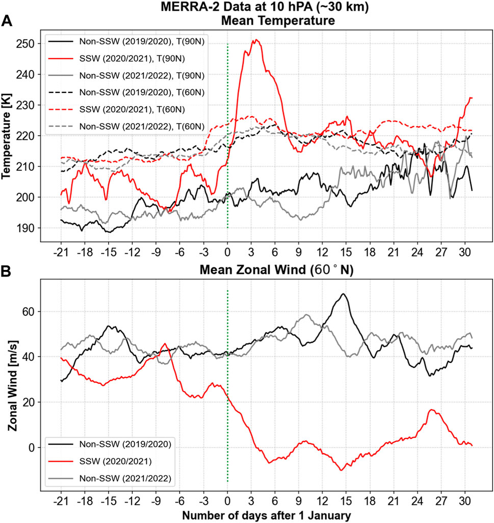
Figure 1. Variation of the zonal mean (A) temperature and (B) zonal winds at 10 hPa (∼30 km) based on MERRA-2; during the 2019/2020 non-SSW winter (black), 2020/2021 SSW winter (red), and 2021/2022 non-SSW winter (gray). The vertical green dashed lines on the day zero marks the onset of the major warming (i.e. 1 January 2021). Mean temperature is shown at the North Pole and at 60^◦N; the mean zonal winds are shown at 60^◦N for the three winters.

Figure 1 demonstrates that, after the onset of the warming on 1 January 2021 (day zero; vertical dashed lines), the Northern polar temperature increases by 40 K–from about 210 K to 250 K, peaking on 5 January 2021. During the ascending phase of the warming, $\bar{u}$ at 60^◦N gradually changes to westward–from $\sim 30$ m s⁻¹ at the onset of the SSW to about −10 m s⁻¹ at the peak phase, demonstrating a reversal of the mean flow direction. The recovery phase of the SSW is relatively long, during which the temperatures remain elevated and $\bar{u}$ is westward compared to the pre-SSW period in December 2020 and during the non-SSW seasons in January 2020 and 2022. It is noticeable that the December 2019 (non-SSW winter) and December 2020 (pre-SSW winter) exhibit some minor differences in mean winds, owing, partially, to interannual variations in planetary wave activity and behavior of large-scale internal waves.

2.2 Choice of analysis period

In order to study thermospheric variations observed by ICON and GOLD during the major SSW, we selected a period centered around the onset of the SSW, i.e., from 6 December 2020 to 26 January 2021 (hereafter called “SSW winter”). The results are compared to those for the non-SSW winter (6 December 2019 to 26 January 2020) in the rest of the paper. The winter of December 2021 to January 2022 was also a non-SSW winter. However, the solar and geomagnetic conditions during this time were greater and more variable (Section 2.3). Since the thermospheric temperatures and winds are closely related to this activity, we only consider the comparison to the non-SSW winter of 6 December 2019 to 26 January 2020. While between ∼90–109 km in the atmosphere both daytime and nighttime ICON wind data are available, only daytime winds are available above ∼109 km up to about 210 km. Therefore, we use only daytime ICON winds from 90–200 km to produce a uniform analysis of the mean wind variations.

2.3 Space weather conditions

Figure 2 shows the geomagnetic and solar conditions in terms of the (a) daily mean A_p index (b) F_10.7 cm solar radio flux, respectively, during the non-SSW (December 2019 - January 2020), the SSW (December 2020 - January 2021), and non-SSW (December 2021 - January 2022) northern winters. The data are from the Geomagnetic Observatory Niemegk, GFZ German Research Centre for Geosciences, Potsdam, Germany (Matzka et al., 2021).

Figure 2

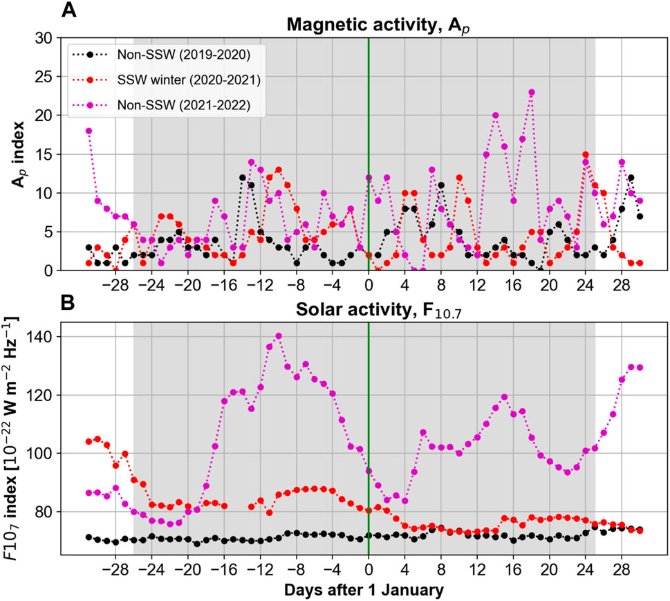
Figure 2. Variation of the (A) geomagnetic activity (A_p) and (B) solar activity (F_10.7) during the 2019/2020 non-SSW (black), 2020/2021 SSW (red), and the 2021/2022 non-SSW (magenta) winters. Vertical green line marks the day zero, which is the onset of the major warming (i.e., 1 January 2021). The gray shading represents the time of the data analysis in this study.

While the space weather conditions are overall relatively quiescent during the winters of 2019–20 and 2020–21, the solar activity during the SSW winter is slightly higher than during the non-SSW winter of 2019–20, since the former corresponds to the ascending phase of the solar activity (Solar Cycle 25), while the latter is the solar minimum (end of Solar Cycle 24).

The observed solar activity during the non-SSW winter of 2021–22 exhibited a significant increase in intensity and variability compared to the previous two winters. This period was characterized by elevated levels of the F_10.7 cm solar radio flux. Given the direct relationship between solar radiation levels and thermospheric heating, such a substantial rise in solar activity significantly influences the energy balance within Earth’s upper atmosphere. Concurrently, the geomagnetic activity during this period demonstrated increased variability. The increased solar irradiance acts as a dominant external forcing mechanism, which could potentially overshadow the more subtle dynamical and thermal responses of the thermosphere to SSWs. In light of these considerations the 2021/2022 non-SSW winter was excluded from the analysis.

Although the magnetic activity is comparable in both the SSW winter and the winter of 2019–20, it exhibits day-to-day variability with occasionally higher activity during the SSW winter than the non-SSW winter, reaching A_p ∼ 12 (K_p ∼ 3 −). In order to reduce the impact of these elevated space weather conditions on our analysis of temperature variations, we have excluded geomagnetically disturbed days in temperature analysis. Accordingly, in the analysis of GOLD temperature (Figure 11) we have removed 5 days in the non-SSW winter and 11 days in the SSW winter, corresponding to days with A_p > 7 (K_p > 2). The grey shading marks the range of the data used for ICON and GOLD analysis (6 December - 26 January in both winters). Before 6 December 2019, ICON horizontal winds are not available and in all our analysis, we have excluded days before 6 December to be consistent in our comparison of the different winters.

2.4 Ionospheric connection explorer (ICON)

ICON’s scientific operation started in December 2019, observing the low-to middle-latitude thermosphere between 10^◦S and ∼40^◦N (Immel et al., 2018) and lasted till 25 November 2022 when contact with the spacecraft was lost. Data are available after 6 December 2019, therefore, for both winters, we use the 52-day data from 6 December to 26 January centered around 1 January 2021 (the SSW onset). Here we use the wind velocity observations performed by the Doppler shift measurements of the green line (λ = 557.7 nm). ICON version 5 green line daytime horizontal winds have been binned daily from 90 to 200 km altitude, including data with solar zenith angles less than 80^◦ (i.e., χ < 80^◦) to exclude solar terminator effects. Also, bins with less than 50 data points have been excluded to avoid low statistical significance. We concentrated our analysis on the Northern Hemisphere low-to middle-latitudes (0^◦–40^◦N).

Recently, validation of the ICON/MIGHTI green line winds have been successfully performed (Makela et al., 2021) and the mean horizontal winds and the associated circulation patterns in the Northern Hemisphere during solstice were characterized (Yiğit et al., 2022).

The associated latitude-local time coverage by ICON at ∼100 km is shown in Figure 3 as well as the latitude-longitude coverage at around 151 km in Figure 4. ICON’s latitude-local time coverage varies from month to month. Therefore, it would be inconsistent to compare the monthly mean fields. It is for this reason we have analyzed the altitude-time variations considering only daytime measurements. For the daytime winds, nearly all longitudes except a narrow band at 300^◦ longitude from 0–10^◦N is not covered during the analyzed months. However, the latitude-longitude coverage between the non-SSW and the SSW winters are very similar. The typical uncertainties in MIGHTI green line wind measurements are 8.7–10 m s⁻¹ (Englert et al., 2017).

Figure 3

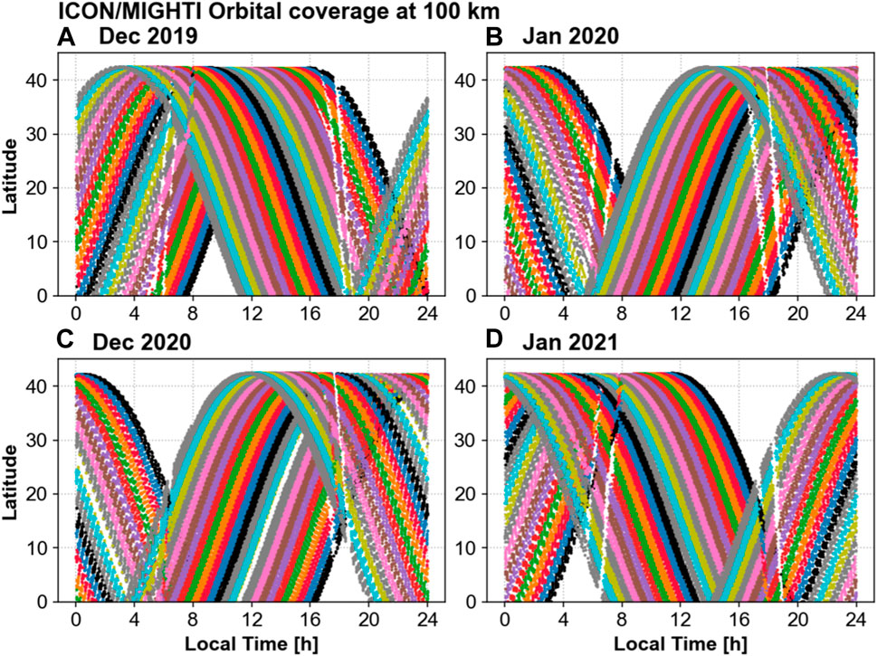
Figure 3. ICON latitude-local time coverage for the non-SSW (December 2019–January 2020) and SSW winters (December 2020–January 2021). The different colors in each panel represent a different day. White spaces show the lack of coverage. (A) Dec 2019. (B) Jan 2020. (C) Dec 2020. (D) Jan 2021.

Figure 4

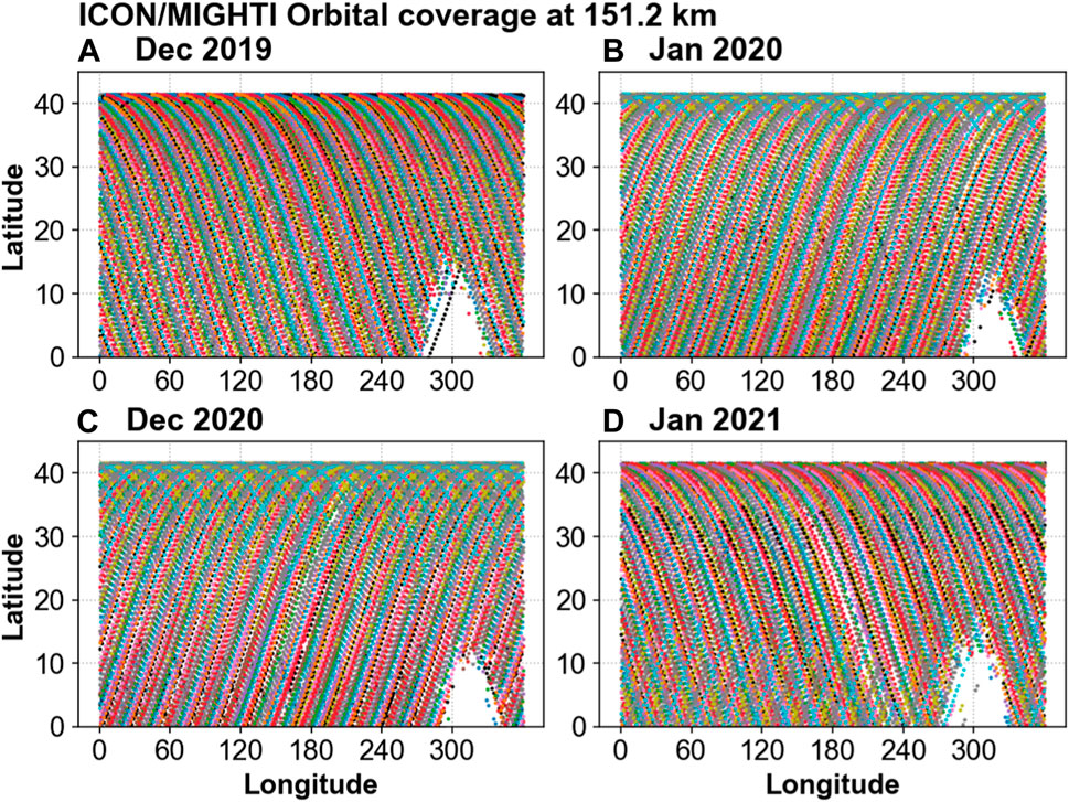
Figure 4. ICON latitude-longitude time coverage for the non-SSW (December 2019–January 2020) and SSW winters (December 2020–January 2021) at around 151 km for the daytime measurements. The different colors in each panel represent a different day. White spaces show the lack of coverage. (A) Dec 2019. (B) Jan 2020. (C) Dec 2020. (D) Jan 2021.

For each day, ICON wind files include around 2,100–2,200 profiles, measured every 22–80 s. This gives more than 110,000 profiles over 52 days for daytime and nighttime together. Since we included only daytime winds with solar zenith angles χ < 80, we included approximately half of the number of total profiles, i.e., 52,000 profiles for the 52-day period studied in a given winter. For the daytime data included here, the profiles are available typically every 27–37 s. In order to improve the data quality in our analysis we have excluded data with the quality flag less (called “wq”) than 0.5, i.e., wq < 0.5, and winds speeds with magnitudes greater than 350 m/s.

In the analysis of the longitudinally averaged daytime zonal and meridional winds in Results (Figures 6, 7), the ICON winds are averaged within each latitude sector, i.e., 0–20^◦ and 20–40^◦N, in 5 km × 1 day altitude-time bins, by including daytime data with χ < 80^◦ and all longitudes. Since southern latitudes were not included, our analysis exclude the South Atlantic Anomaly.

2.5 Global-Scale Observations of the Limb and Disk (GOLD)

GOLD observes the Far Ultraviolet (FUV) spectrum of Earth’s atmosphere at geostationary orbit, from 0610 to 0040 Universal Time (UT) every day, providing, among others, daytime thermospheric temperatures near 150 km at low- and midlatitudes (0^◦ to ±60^◦), depending on the solar zenith angle.

The temporal resolution of the GOLD temperatures is about 30 min. The longitudes covered by GOLD range from −100^◦ to 10^◦. Similar to ICON, we have used 52 days of GOLD data centered around 1 January. Thermospheric temperatures are retrieved from the daytime disk scan measurements. The effective disk neutral temperatures (T_disk) are derived from the N₂ Lyman-Birge-Hopfield (LBH) emission profile at a height of approximately 150 km. The T_disk data product is created from spatial-spectral image cubes from the disk scans (Level 1C data). These pixels are binned 2^◦ × 2^◦ spatially, resulting in a data product that has a spatial resolution (nadir) of 250 km × 250 km, with a precision of ±55 km (Eastes et al., 2020). We use version 4 of the level 2 T_disk data product. The longitude-latitude grids are fixed for all scans. The T_disk data file has flags for data quality issues at the file and pixel levels. Observations with dqi $>$ 0 at both levels are not considered in our analysis. To increase signal-to-noise ratio (SNR), observations of χ > 65^◦ have been removed. Random errors in the 2 × 2 binned data vary with SNR of the N₂ LBH emission and ranges from 20 (for high SNR) to 90 K (for low SNR). Figure 5 shows the spatiotemporal coverage for 2 representative days, 31 December 2019 and 31 December 2020, during the non-SSW winter and SSW winter, respectively. The coverage represents the good quality retained T_disk temperature profiles. In panels (d) and (i), an uneven latitude versus SZA (χ) distribution is seen. Higher latitudes are covered at higher χ′s, which has implications for the observed temperatures. Otherwise, there is an even χ coverage across all longitudes. Two successive years were chosen to demonstrate the negligible amount of variability between the 2 years in terms of the orbital coverage.

Figure 5

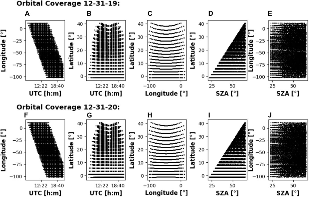
Figure 5. GOLD spatiotemporal coverage for retained T_disk data profiles. Panels (A–E) demonstrate the coverage for 31 December 2019 and panels (F–J) demonstrate the coverage for 31 December 2020.

In Figure 11G in the main text, a linear model was fitted to the data for each of the latitude bands in order to better visualize the variability. The standard deviation of the residuals were then used to generate the error bars in the plot, rather than the standard deviation of the raw temperature data. Therefore, the error bars in the plot should be interpreted as indicating the variability around the fitted linear trend, rather than the absolute variability in temperature.

3 Results and discussion

3.1 Observations of thermospheric horizontal winds

In order to assess changes in the thermospheric winds induced by the major SSW, we consider ICON/MIGHTI measurements for two periods with a common spatiotemporal coverage. Figures 6, 7 present the daily evolution of the daytime longitudinally averaged (i.e., zonal mean) zonal and meridional winds, respectively, during the major SSW (December 2020—January 2021) and non-SSW winters (December 2019—January 2020) at two representative latitude bands: at low-latitude (0–20^◦N, left column) and low-to midlatitude (20^◦ - 40^◦N, right column) regions. Altitudes and days, for which observations are not available, are shown in gray shading.

Figure 6

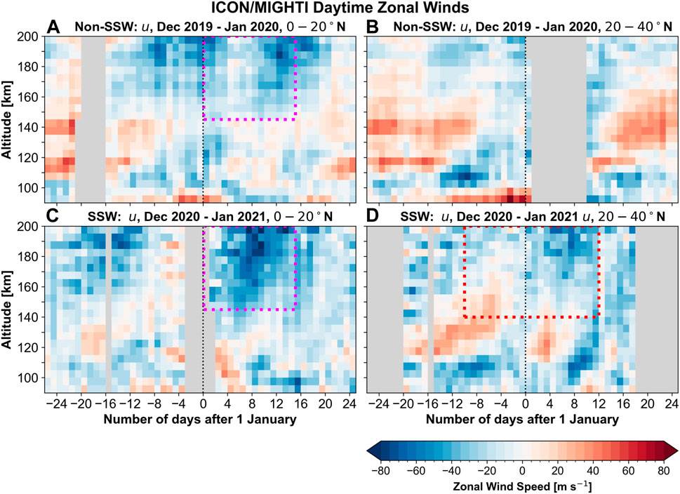
Figure 6. Contour plots of the daytime mean zonal winds in m/s during the non-SSW winter (December 2019-January 2020, first row) and SSW winter (December 2020-January 2021, second row) plotted from 6 December to 26 January at two latitude bands, 0–20^◦N (left column, panels (A, C)) and 20–40^◦N (right column, panels (B, D)). The same color scales are used for all winds. Red/blue shadings (positive/negative values) represent eastward/westward winds. The vertical black dashed lines mark the onset of the warming (1 January 2021), where the warming onset is also marked in non-SSW winter plots for comparison. Gray shading designates data gaps. At 0–20^◦N, the zonal winds (purple boxes, panels (A, C) during non SSW year are compared to their values during the SSW year in January. At 20–40^◦N the post-SSW period is compared with the pre-SSW one for zonal (red box, panel (D).

Figure 7

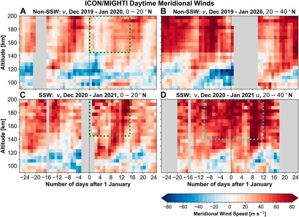
Figure 7. Same as Figure 6 but for the meridional winds. Red/blue shadings (positive/negative values) represent northward/southward winds. At 0–20^◦N, the meridional winds (green boxes, panels (A, C) during non SSW year are compared to their values during the SSW year in January. At 20–40^◦N the post-SSW period is compared with the pre-SSW one for meridional winds (cyan box, panel (D).

Even without an SSW, the observed thermospheric horizontal winds exhibit a significant degree of day-to-day variability. This could be related to a combination of physical processes, such as a) changes in the dynamics of internal atmospheric waves, b) variability of the solar and geomagnetic activity, and c) orbital effects, e.g., ICON’s orbit precession toward earlier local times by about 29.8 min every day (Figure 3). Under the non-SSW conditions (during the non-SSW winter and before the onset of the warming), the daytime zonal winds exhibit an alternating with altitude pattern at low- and low-to midlatitudes: typically eastward in the upper mesosphere, westward in the lower thermosphere and eastward again above ∼ 120 km. Above ∼160 km, the westward flow dominates, in general. The daytime meridional winds without an SSW are overall northward (representing the poleward, summer-to-winter circulation) in the upper mesosphere, southward (winter-to-summer transport) in the lower thermosphere, and poleward again above ∼130 km (Figures 6A,B; Figure 7A,B).

In the winter hemisphere, westward propagating GWs, owing to their faster intrinsic horizontal phase speeds ${\widehat{c}}_i$, have favorable upward propagation conditions through the mean eastward stratomesospheric jets, maintained by the Coriolis torque. Saturation of the surviving harmonics produces momentum flux divergences (i.e., GW drag) in the MLT that reverses the zonal winds from eastward to westward and the meridional winds from northward to southward around 90–110 km (Garcia and Solomon, 1985; Yiğit et al., 2009; 2021).

Secondary or higher-order waves can be generated in the middle atmosphere by the dissipation of the primary waves (Holton and Alexander, 1999). Secondary waves could thus contribute to the momentum balance in the MLT and above, as suggested by previous theoretical modeling studies (Vadas et al., 2018), however, based on first-principle theoretical arguments, the relative contribution of secondary waves to the momentum balance is generally expected to be much smaller than those of primary waves (Medvedev et al., 2023). Nevertheless, a number of observational studies consider secondary waves as important contributor to the momentum fluxes in the MLT region. Vincent et al. (2013) studied gravity wave absolute momentum fluxes with meteor radars and stated that they could not distinguish primary from the secondary waves, but nevertheless discussed the potential importance of secondary waves. Secondary waves were also considered as a complicating factor in that study. More recently, de Wit et al. (2017) argued that the large eastward MLT GW momentum fluxes observed near the Southern Andes could not be explained by the direct upward propagating orographic waves and thus were likely caused by secondary gravity waves. Kogure et al. (2020) used two satellites to study mountain wave breaking over the Andes and their connection to secondary waves. They concluded that ring-like concentric waves above the wave breaking region were associated with secondary wave generation. The momentum forcing is also supplemented by upward propagating diurnal and semidiurnal tides at low- and middle-latitudes, respectively (Jones et al., 2019; Miyoshi and Yiğit, 2019; Griffith et al., 2021; Conte et al., 2024).

Changes in the stratosphere during SSWs can be communicated to upper layers of the atmosphere via changes in the large-scale structure and in upward propagation and dissipation conditions of internal waves. The degree of vertical coupling during SSWs can be in general different than during quiescent times. After the onset of the warming in January 2021 (Figures 6C,D, 7C,D), westward (negative) and northward (positive) winds relatively strengthen depending on the altitude and day, especially above 140 km. The dotted color boxes are thought to aid with the comparison of the wind changes due to the SSW. There is an indication that the thermospheric winds begin to change before the start of the SSW, which can probably be related to the fact that the stratospheric mean zonal wind decrease precedes the polar temperature rise by several days (Figure 1B). This phenomenon is known to modulate upward gravity wave propagation (Yiğit and Medvedev, 2012; Miyoshi et al., 2015).

Figure 8 analyzes SSW-induced changes in horizontal winds by subtracting the 7-day averaged winds before the onset of the SSW (i.e., 25–31 December 2020) from the rest of the wind observations in the 2020/2021 SSW winter. Difference winds are shown for the zonal (Δu) and meridional (Δv) components. Overall, post-SSW winds are more westward and northward relative to the pre-SSW period. Figure 9 plots the averaged horizontal circulation in terms of vectors during the pre-SSW and post-SSW periods, focusing on an altitude interval of 140–160 km and a time window of 1 week with respect to the SSW onset in each case. This representation shows more clearly the westward turning of the horizontal circulation during the SSW, especially at low-latitudes.

Figure 8

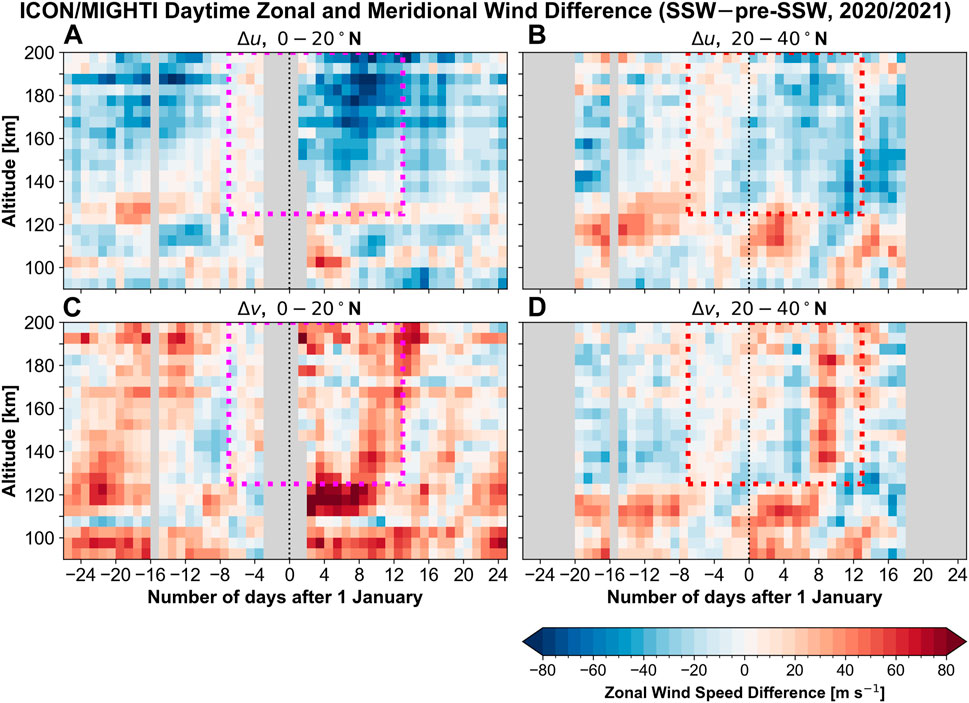
Figure 8. Zonal (first row, panels A, C) and meridional (second row, panels C, D) wind differences as calculated by subtracting the 7-day averaged pre-SSW winds (1 week before the SSW onset, i.e., 25–31 December 2021) from the rest of the wind observations, i.e., SSW–pre-SSW, at 0–20^◦N (left) and at 20–40^◦N (right).

Figure 9

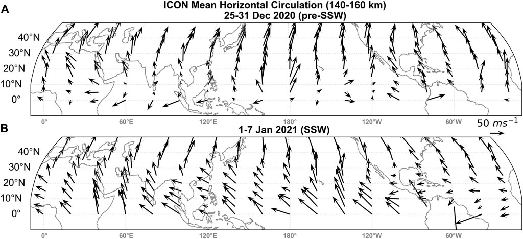
Figure 9. Latitude-longitude distribution of the averaged horizontal wind circulation during the pre-SSW period (1 week before the SSW onset, i.e., 25–31 December 2020, panel (A)) and during the SSW (1–7 January 2021, panel (B)) within a representative thermospheric altitude range of 140–160 km as observed by ICON/MIGHTI. The wind vectors are represented with respect to the 50 m s⁻¹ wind speed.

3.2 Tidal activity during the major SSW

Diurnal and semidiurnal tides with long vertical wavelengths can reach upper mesospheric and thermospheric altitudes and play an important role in the momentum budget of the low-to midlatitude thermosphere (Jones et al., 2019; Miyoshi and Yiğit, 2019; Forbes et al., 2022). Given the different general mechanism and spatiotemporal characteristics of the different tides, the response of the upper atmosphere across the tidal spectrum is expected to vary. In other words, the different parts of the tidal spectrum can be modulated by the SSW to different amounts. Figure 10 presents the latitude-time distributions of the semidiurnal tidal amplitudes for the SW2, SW1, and SW3 (left panels) during the SSW year, as well as for the diurnal components, DW1, D0, and DE3 (right panels), as retrieved from ICON zonal winds at around 100 km. It is seen that the SW2 is the strongest component compared to the others and it is enhanced at low-latitudes after the onset of the major warming. Previous studies suggested that the SW2 is strong after many split-type SSWs (Ma et al., 2023), which could be also related to the stationary planetary wave-2 (SPW2) induced by splitting vortices after the associated SSWs (Ma et al., 2020).

Figure 10

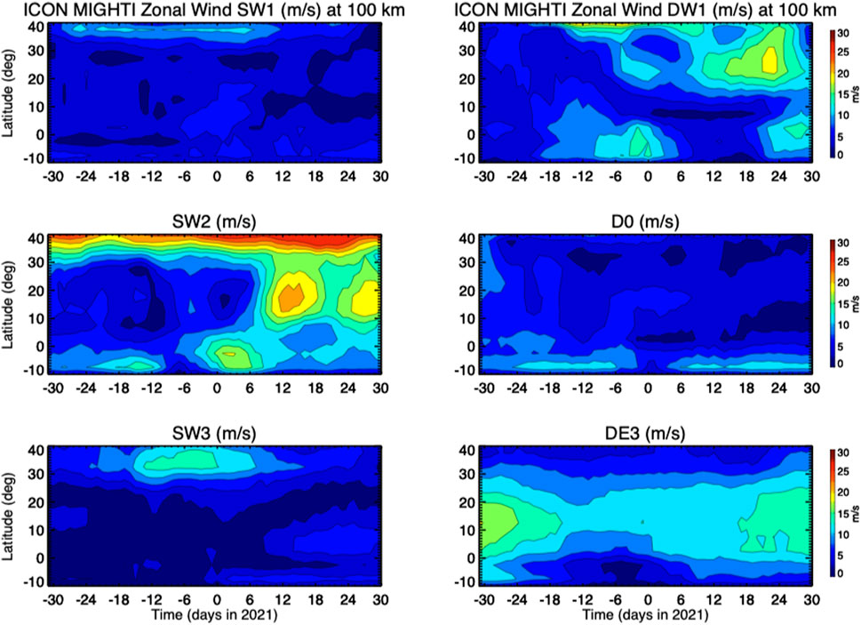
Figure 10. Latitude-time distributions of the amplitudes of the semidiurnal components, SW2, SW1, and SW3 (left panels) as well as the diurnal components, DW1, D0, and DE3 (right panels), as retrieved from ICON zonal winds at around 100 km. Day zero marks the onset of the warming, i.e., 1 January 2021.

Zhang et al. (2022) studied the semidiurnal tides using Hough mode extension of the zonal and meridional winds and emphasized the importance of semidiurnal tides in the variations of equatorial plasma drifts and neutral winds during the SSW. Overall, our results are in good agreement with previous findings of the enhanced semidiurnal migrating tides in the low- and midlatitude lower and upper thermosphere during SSWs (Goncharenko et al., 2010b; Liu et al., 2013; Oberheide, 2022).

3.3 Observations of thermospheric temperature

Figure 11 presents the day-to-day evolution of the daytime neutral temperatures near 150 km as measured by GOLD, and averaged longitudinally and over the same two representative latitude bands discussed above. Based on GOLD’s coverage, only longitudes between 100^◦W and 10^◦E contributed to the zonal mean. The upper two rows (Figures 11A–D) show the temperature variations as a function of solar zenith angle χ. Note that the two latitude bands have different χ coverage. The observations for 25^◦ < χ < 65^◦ contributed to the low-latitude 0–20^◦N band, with a larger portion of measurements centered around 65^◦. The low-to midlatitude (20^◦ - 40^◦N) band includes observations for χ between 45^◦ and 65^◦, with a larger portion taken around χ = 55^◦. Rows three and four (Figures 11E,F) display another aspect of temperature variations: the latitude-time cross-sections at 150 km during the non-SSW and SSW winters, respectively. It is seen that, at all latitudes and solar zenith angles, thermospheric temperatures drop during the SSW. The cooling trend begins shortly before the SSW onset and lasts for about 15 days. The thermospheric cooling is more clearly seen in Figure 11G, which presents the day-to-day variations of the average temperature in the corresponding latitude bands. The error bars indicate the variability around a fitted linear trend (Section 2.5). Starting a few days before the onset of the SSW, the thermospheric temperature decreases by about 50 K, from ∼730 K–680 K, after which it returns back to ∼720 K over about 10 days. Such cooling trend is untypical in the low-latitude thermosphere in the absence of SSWs, as a comparison with the non-SSW winter shows. It is also seen that the thermosphere is much colder during the non-SSW winter, because it coincided with the solar minimum.

Figure 11

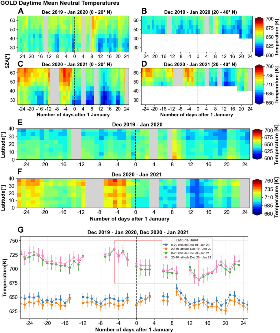
Figure 11. Contour plots of daytime neutral temperatures in K during the non-SSW winter (December 2019-January 2020, first and third rows) and SSW winter (December 2020-January 2021, second and fourth rows) plotted from 6 December to 26 January. Panels (A–D) are plotted with respect to the solar zenith angle (SZA) for two latitude bands, 0–20^◦N (left column) and 20–40^◦N (right column). Panels (E, F) are presented as a function of latitude. The light grey shading represents the removed days with A_p index greater than 7. The white shading represents missing data. Panel (G) shows the variation of the neutral temperature at different latitude bands. Both SSW and non-SSW winters’ temperature average over the respective latitude bands–blue/orange colors (0–20^◦N/20–40^◦N) represent the non-SSW winter, and green/pink colors (0–20^◦N/20–40^◦N) represent the SSW winter. The vertical black dashed lines mark the onset of the warming (1 January 2021). Warming onset is also marked in non-SSW winter for comparison. Error bars are ± σ of regression residuals.

3.4 Mechanisms of thermal changes and connections to winds in the low-latitude thermosphere

Observations presented above demonstrate a global response of the low-to middle-latitude thermosphere to the major SSW event. Generally, winds and neutral temperature are affected by a number of physical processes pertaining to external (space weather, or coupling from above) and internal forcing (coupling from below) (Yiğit et al., 2016). SSWs, which originate in the troposphere and lower stratosphere, are significant disturbances of the latter region. They quickly modulate the vertical propagation of internal atmospheric gravity waves and solar tides, which have a broad spectrum and can reach thermospheric altitudes with significant amplitudes. A number of observational and modeling studies found that the thermospheric GW activity decreases after a major warming is fully developed (Miyoshi et al., 2015; Nayak and Yiğit, 2019). On the other hand, the amplitude of the migrating Sun-synchronous semidiurnal tide increases during SSWs in the low- and midlatitude lower and upper thermosphere (Goncharenko et al., 2010b; Liu et al., 2013; Oberheide, 2022). More recently, Gasperini et al. (2023) analyzed ICON green line winds in the MLT, showing that the SW2 zonal wind amplitudes are amplified following the 2020/2021 major SSW, which we were able to confirm in our analysis (Section 3.2). These two changes can be related, because GWs are known to attenuate the semidiurnal tide in the thermosphere (Miyoshi and Yiğit, 2019). That is, a decrease in gravity wave activity could provide favorable conditions for SW2 tidal propagation and growth. Semidiurnal tidal sources can also be modulated owing to a redistribution of the stratospheric ozone (Pancheva et al., 2003). Thus, the modified wave forcing can directly affect the residual circulation in the thermosphere (Koval et al., 2021). Coupled changes in gravity wave and tidal activity are the probable cause for the observed wind variations in thermospheric altitudes. Systematic modeling studies are required for isolating the effects of gravity waves and semidiurnal tides (and their possible interactions) during major stratospheric warmings.

SSW-induced thermal and dynamical changes are intimately connected. In addition to direct wave forcing, thermodynamical changes can be caused by modification of the large-scale flow. Vertical motions and the associated adiabatic heating/cooling are connected to divergence and convergence of horizontal winds via continuity (Rishbeth et al., 1969). Previous research demonstrated significant low-latitude thermospheric cooling during major SSWs. During the January 2009 SSW, Liu et al. (2011) discovered large density drops in GRACE and CHAMP observations above 325 km, which corresponded to a ∼50 K cooling. Using simulations with a whole atmosphere model, Liu et al. (2013) reported a net cooling of the thermosphere above 100 km during the 2009 major SSW. Although the spatiotemporal coverage between previous studies and our analysis is somewhat different, our results are qualitatively in agreement with previous findings and contribute toward filling the gap in vertical coupling between the troposphere and the upper atmosphere. A net upwelling and enhanced poleward flow initiated by SSW-induced changes can account for the observed cooling in the low-latitude thermosphere around 150 km. However, demonstration of this physical mechanism would require three-dimensional global modeling effort, such as the one conducted by Miyoshi et al. (2015). Overall, our findings are complementary to previous studies that showed upper thermospheric cooling associated with upwelling at low-latitudes using CHAMP and GRACE satellites (Liu et al., 2013; 2011). It was later studied in more detail using whole atmosphere models, which demonstrated that the cooling extends to middle thermospheric altitudes (Liu et al., 2014; Miyoshi et al., 2015).

Finally, a subtle decrease of solar activity (from 85 to 75 × 10⁻²² W m⁻² s⁻¹) over the SSW period (Figure 2) can contribute to some extent to the observed 50 K temperature drop around 150 km. Tests with the NRLMSIS empirical model (Picone et al., 2002) however suggest that a reduction of the solar activity by ten F_10.7 radio flux units changes temperature by only 5–10 K around 150 km altitude (not shown). Obviously, more accurate and self-consistent estimates can be obtained using models extending from the lower to the upper atmosphere or even better whole atmosphere general circulation models.

4 Summary and conclusion

Combining ICON and GOLD satellite observations, we have explored the impact of the 2020/2021 major sudden stratospheric warming (SSW) on the thermospheric horizontal circulation (i.e., zonal and meridional winds) between 90 and 200 km and temperatures around 150 km. Wind and temperature variations during the SSW have been compared to the pre- and non-SSW periods. The main inferences of our study are as follows:

1. ICON daytime longitudinally averaged zonal winds at low-to midlatitude are typically eastward in the upper mesosphere; reverse their direction to westward in the lower thermosphere, and change again to eastward above ∼120 km. Above ∼160 km, the westward flow dominates, in general. Daytime longitudinally averaged meridional winds are overall northward (poleward, representing the summer-to-winter transport) in the upper mesosphere, southward (equatorward, or winter-to-summer flow) in the lower thermosphere, and poleward again above ∼130 km.

2. After the onset of the major warming, westward and northward winds strengthen depending on the altitude and day, especially above 140 km. There is an indication that the thermospheric winds begin to change before the start of the SSW.

3. ICON observations show that the semidiurnal migrating tides (SW2) are enhanced at low-latitudes after the onset of the major SSW. It was seen that the SW2 is the strongest tides compared to other semidiurnal (SW1, SW3) and diurnal (D0, DW1, DE3) components. Previous studies have indicated that gravity waves can damp the SW2 and the thermospheric gravity wave activity decreases during the major SSW, thus it is possible that weaker gravity wave activity can contribute to the enhancement of the SW2 in the thermosphere during the major warming.

4. The low-latitude thermosphere cools down during the SSW by about 50 K. The cooling trend starts about 7–10 days before the onset of the warming in the stratosphere and lasts for about 2 weeks. The recovery phase of the temperature takes about 10 days.

5. SSW-induced thermal and dynamical changes are intimately connected. A net upwelling and enhanced poleward flow initiated by SSW-induced changes can account for the observed cooling in the low-latitude thermosphere around 150 km, as has been supported by previous general circulation modeling studies (e.g., Liu et al., 2014). Thus, the observed temperature drop in the thermosphere is likely caused by adiabatic cooling associated with changes in the large-scale horizontal flow.

6. Our findings of low-latitude cooling during the 2020/2021 major warming are complementary to previous studies that showed upper thermospheric cooling associated with upwelling at low-latitudes using CHAMP and GRACE satellites.

Finally, we note that, while comparing different years, data coverage and quality issues can obstruct distinguishing SSW-induced thermospheric changes from the changes caused by inter-annual variability. Also, most of the conclusions of this study are based on the comparisons between the 2019/2020 non-SSW winter and the 2020/2021 SSW winter.

Data availability statement

The original contributions presented in the study are included in the article/Supplementary Materials, further inquiries can be directed to the corresponding author. The MIGHTI horizontal wind data (version 5) used in this study are available at the ICON data center (https://icon.ssl.berkeley.edu/Data). The GOLD level 2 data used in this study are available at the GOLD Science Data Center (https://gold.cs.ucf.edu/search/) and at NASA’s Space Physics Data Facility (https://spdf.gsfc.nasa.gov/pub/data/gold/level2/tdisk).

Author contributions

EY: Conceptualization, Data curation, Formal Analysis, Funding acquisition, Investigation, Methodology, Project administration, Resources, Software, Supervision, Validation, Visualization, Writing–original draft, Writing–review and editing. AG: Formal Analysis, Writing–original draft, Writing–review and editing. AM: Writing–original draft, Writing–review and editing. FG: Writing–original draft, Writing–review and editing. QW: Writing–original draft, Writing–review and editing. NS: Writing–original draft, Writing–review and editing.

Funding

The author(s) declare that financial support was received for the research, authorship, and/or publication of this article. This work was supported by NASA (Grant 80NSSC22K0016) and National Science Foundation (NSF) (Grant AGS 20330046). ICON is supported by NASA’s Explorers Program through contracts NNG12FA45C and NNG12FA42I.

Conflict of interest

FG was employed by Orion Space Solutions.

The remaining authors declare that the research was conducted in the absence of any commercial or financial relationships that could be construed as a potential conflict of interest.

The author(s) declared that they were an editorial board member of Frontiers, at the time of submission. This had no impact on the peer review process and the final decision.

Publisher’s note

All claims expressed in this article are solely those of the authors and do not necessarily represent those of their affiliated organizations, or those of the publisher, the editors and the reviewers. Any product that may be evaluated in this article, or claim that may be made by its manufacturer, is not guaranteed or endorsed by the publisher.

References

Azeem, I., Crowley, G., and Honniball, C. (2015). Global ionospheric response to the 2009 sudden stratospheric warming event using Ionospheric Data Assimilation Four-Dimensional (IDA4D) algorithm: ionosphere during Stratospheric Warming. J. Geophys. Res. Space Phys. 120, 4009–4019. doi:10.1002/2015JA020993

CrossRef Full Text | Google Scholar

Butler, A. H., Seidel, D. J., Hardiman, S. C., Butchart, N., Birner, T., and Match, A. (2015). Defining sudden stratospheric warmings. Bull. Am. Meteorological Soc. 96, 1913–1928. doi:10.1175/BAMS-D-13-00173.1

CrossRef Full Text | Google Scholar

Conte, J. F., Chau, J. L., Yiğit, E., Suclupe, J., and Rodríguez, R. (2024). Investigation of mesosphere and lower thermosphere dynamics over central and northern Peru using SIMONe systems. J. Atmos. Sci. 81, 93–104. doi:10.1175/JAS-D-23-0030.1

CrossRef Full Text | Google Scholar

de Wit, R. J., Janches, D., Fritts, D. C., Stockwell, R. G., and Coy, L. (2017). Unexpected climatological behavior of MLT gravity wave momentum flux in the lee of the Southern Andes hot spot. Geophys. Res. Lett. 44, 1182–1191. doi:10.1002/2016GL072311

CrossRef Full Text | Google Scholar

Eastes, R. W., McClintock, W. E., Burns, A. G., Anderson, D. N., Andersson, L., Aryal, S., et al. (2020). Initial observations by the GOLD mission. J. Geophys. Res. Space Phys. 125, e2020JA027823. doi:10.1029/2020JA027823

CrossRef Full Text | Google Scholar

Englert, C. R., Harlander, J. M., Brown, C. M., Marr, K. D., Miller, I. J., Stump, J. E., et al. (2017). Michelson interferometer for global high-resolution thermospheric imaging (MIGHTI): instrument design and calibration. Space Sci. Rev. 212, 553–584. doi:10.1007/s11214-017-0358-4

PubMed Abstract | CrossRef Full Text | Google Scholar

Forbes, J. M., Oberheide, J., Zhang, X., Cullens, C., Englert, C. R., Harding, B. J., et al. (2022). Vertical coupling by solar semidiurnal tides in the thermosphere from ICON/MIGHTI measurements. J. Geophys. Res. Space Phys. 127, e2022JA030288. doi:10.1029/2022JA030288

CrossRef Full Text | Google Scholar

Garcia, R. R., and Solomon, S. (1985). The effect of breaking gravity waves on the dynamics and chemical composition of the mesosphere and lower thermosphere. J. Geophys. Res. 90, 3850–3868. doi:10.1029/JD090iD02p03850

CrossRef Full Text | Google Scholar

Gasperini, F., Crowley, G., Immel, T. J., and Harding, B. J. (2022). Vertical wave coupling in the low-latitude ionosphere-thermosphere as revealed by concurrent ICON and COSMIC-2 observations. Space Sci. Rev. 218, 55. doi:10.1007/s11214-022-00923-1

CrossRef Full Text | Google Scholar

Gasperini, F., Jones, M., Harding, B. J., and Immel, T. J. (2023). Direct observational evidence of altered mesosphere lower thermosphere mean circulation from a major sudden stratospheric warming. Geophys. Res. Lett. 50, e2022GL102579. doi:10.1029/2022GL102579

CrossRef Full Text | Google Scholar

Gavrilov, N. M., Koval, A. V., Pogoreltsev, A. I., and Savenkova, E. N. (2018). Simulating planetary wave propagation to the upper atmosphere during stratospheric warming events at different mountain wave scenarios. Adv. Space Res. 61, 1819–1836. doi:10.1016/j.asr.2017.08.022

CrossRef Full Text | Google Scholar

Gavrilov, N. M., and Kshevetskii, S. P. (2015). Dynamical and thermal effects of nonsteady nonlinear acoustic-gravity waves propagating from tropospheric sources to the upper atmosphere. Adv. Space Res. 56, 1833–1843. doi:10.1016/j.asr.2015.01.033

CrossRef Full Text | Google Scholar

Goncharenko, L. P., Chau, J. L., Liu, H.-L., and Coster, A. J. (2010a). Unexpected connections between the stratosphere and ionosphere. Geophys. Res. Lett. 37, n/a. doi:10.1029/2010GL043125

CrossRef Full Text | Google Scholar

Goncharenko, L. P., Coster, A. J., Chau, J. L., and Valladares, C. E. (2010b). Impact of sudden stratospheric warmings on equatorial ionization anomaly. J. Geophys. Res. 115, n/a. doi:10.1029/2010JA015400

CrossRef Full Text | Google Scholar

Goncharenko, L. P., Harvey, V. L., Liu, H., and Pedatella, N. M. (2021). Sudden stratospheric warming impacts on the ionosphere–thermosphere system. Ionos. Dyn. Appl. Am. Geophys. Union AGU chap. 16, 369–400. doi:10.1002/9781119815617.ch16

CrossRef Full Text | Google Scholar

Gong, Y., Zhou, Q., Zhang, S., Aponte, N., and Sulzer, M. (2016). An incoherent scatter radar study of the midnight temperature maximum that occurred at Arecibo during a sudden stratospheric warming event in January 2010. J. Geophys. Res. Space Phys. 121, 5571–5578. doi:10.1002/2016JA022439

CrossRef Full Text | Google Scholar

Griffith, M. J., Dempsey, S. M., Jackson, D. R., Moffat-Griffin, T., and Mitchell, N. J. (2021). Winds and tides of the Extended Unified Model in the mesosphere and lower thermosphere validated with meteor radar observations. Ann. Geophys. 39, 487–514. doi:10.5194/angeo-39-487-2021

CrossRef Full Text | Google Scholar

Gu, S., Hou, X., Qi, J., TengChen, K., and Dou, X. (2020). Reponses of middle atmospheric circulation to the 2009 major sudden stratospheric warming. Earth Planet. Phys. 4, 1–7. doi:10.26464/epp2020046

CrossRef Full Text | Google Scholar

Holton, J. R. (1976). A semi-spectral numerical model for wave-mean flow interactions in the stratosphere: application to sudden stratospheric warmings. J. Atmos. Sci. 33, 1639–1649. doi:10.1175/1520-0469(1976)033<1639:assnmf>2.0.co;2

CrossRef Full Text | Google Scholar

Holton, J. R., and Alexander, M. J. (1999). Gravity waves in the mesosphere generated by tropospheric convention. Tellus A Dyn. Meteorology Oceanogr. 51, 45. doi:10.3402/tellusa.v51i1.12305

CrossRef Full Text | Google Scholar

Immel, T. J., England, S. L., Mende, S. B., Heelis, R. A., Englert, C. R., Edelstein, J., et al. (2018). The ionospheric connection explorer mission: mission goals and design. Space Sci. Rev. 214, 13. doi:10.1007/s11214-017-0449-2

PubMed Abstract | CrossRef Full Text | Google Scholar

Jones, M., Forbes, J. M., and Sassi, F. (2019). The effects of vertically propagating tides on the mean dynamical structure of the lower thermosphere. J. Geophys. Res. Space Phys. 124, 7202–7219. doi:10.1029/2019JA026934

CrossRef Full Text | Google Scholar

Karpov, I. V., Bessarab, F. S., Borchevkina, O. P., Artemenko, K. A., and Klopova, A. I. (2018). Modeling the effect of mesospheric internal gravity waves in the thermosphere and ionosphere during the 2009 sudden stratospheric warming. Geomagn. Aeron. 58, 509–522. doi:10.1134/S0016793218040084

CrossRef Full Text | Google Scholar

Kogure, M., Yue, J., Nakamura, T., Hoffmann, L., Vadas, S. L., Tomikawa, Y., et al. (2020). First direct observational evidence for secondary gravity waves generated by mountain waves over the Andes. Geophys. Res. Lett. 47, e2020GL088845. doi:10.1029/2020GL088845

CrossRef Full Text | Google Scholar

Koucká Knížová, P., Laštovička, J., Kouba, D., Mošna, Z., Podolská, K., Potužníková, K., et al. (2021). Ionosphere influenced from lower-lying atmospheric regions. Front. Astron. Space Sci. 8. doi:10.3389/fspas.2021.651445

CrossRef Full Text | Google Scholar

Koval, A. V., Chen, W., Didenko, K. A., Ermakova, T. S., Gavrilov, N. M., Pogoreltsev, A. I., et al. (2021). Modelling the residual mean meridional circulation at different stages of sudden stratospheric warming events. Ann. Geophys. 39, 357–368. doi:10.5194/angeo-39-357-2021

CrossRef Full Text | Google Scholar

Laskar, F. I., McCormack, J. P., Chau, J. L., Pallamraju, D., Hoffmann, P., and Singh, R. P. (2019). Interhemispheric meridional circulation during sudden stratospheric warming. J. Geophys. Res. Space Phys. 124, 7112–7122. doi:10.1029/2018JA026424

CrossRef Full Text | Google Scholar

Liu, H., Doornbos, E., Yamamoto, M., and Tulasi Ram, S. (2011). Strong thermospheric cooling during the 2009 major stratosphere warming. Geophys. Res. Lett. 38. doi:10.1029/2011GL047898

CrossRef Full Text | Google Scholar

Liu, H., Jin, H., Miyoshi, Y., Fujiwara, H., and Shinagawa, H. (2013). Upper atmosphere response to stratosphere sudden warming: local time and height dependence simulated by GAIA model. Geophys. Res. Lett. 40, 635–640. doi:10.1002/grl.50146

CrossRef Full Text | Google Scholar

Liu, H., Miyoshi, Y., Miyahara, S., Jin, H., Fujiwara, H., and Shinagawa, H. (2014). Thermal and dynamical changes of the zonal mean state of the thermosphere during the 2009 SSW: GAIA simulations. J. Geophys. Res. Space Phys. 119, 6784–6791. doi:10.1002/2014JA020222

CrossRef Full Text | Google Scholar

Ma, H., Liu, L., He, M., Yu, Y., Zhang, R., Lyu, H., et al. (2023). The evolution of solar tide-like signatures in the ionospheric total electron content during major sudden stratospheric warming events. J. Geophys. Res. Space Phys. 128, e2023JA031979. doi:10.1029/2023JA031979

CrossRef Full Text | Google Scholar

Ma, Z., Gong, Y., Zhang, S., Luo, J., Zhou, Q., Huang, C., et al. (2020). Comparison of stratospheric evolution during the major sudden stratospheric warming events in 2018 and 2019. Earth Planet. Phys. 4, 1–11. doi:10.26464/epp2020044

CrossRef Full Text | Google Scholar

Makela, J. J., Baughman, M., Navarro, L. A., Harding, B. J., Englert, C. R., Harlander, J. M., et al. (2021). Validation of ICON-MIGHTI thermospheric wind observations: 1. Nighttime red-line ground-based fabry-perot interferometers. J. Geophys. Res. Space Phys. 126, e2020JA028726. doi:10.1029/2020JA028726

PubMed Abstract | CrossRef Full Text | Google Scholar

Matsuno, T. (1971). A dynamical model of the stratospheric sudden warming. J. Atmos. Sci. 28, 1479–1494. doi:10.1175/1520-0469(1971)028<1479:admots>2.0.co;2

CrossRef Full Text | Google Scholar

Matzka, J., Stolle, C., Yamazaki, Y., Bronkalla, O., and Morschhauser, A. (2021). The geomagnetic kp index and derived indices of geomagnetic activity. Space weather. 19, e2020SW002641. doi:10.1029/2020SW002641

CrossRef Full Text | Google Scholar

Medvedev, A. S., Klaassen, G. P., and Yiğit, E. (2023). On the dynamical importance of gravity wave sources distributed over different heights in the atmosphere. J. Geophys. Res. Space Phys. 128, e2022JA031152. doi:10.1029/2022JA031152

CrossRef Full Text | Google Scholar

Miyoshi, Y., and Fujiwara, H. (2008). Gravity waves in the thermosphere simulated by a general circulation model. J. Geophys. Res. 113, D01101. doi:10.1029/2007JD008874

CrossRef Full Text | Google Scholar

Miyoshi, Y., Fujiwara, H., Jin, H., and Shinagawa, H. (2015). Impacts of sudden stratospheric warming on general circulation of the thermosphere. J. Geophys. Res. Space Phys. 120 (10), 912. doi:10.1002/2015JA021894

CrossRef Full Text | Google Scholar

Miyoshi, Y., and Yiğit, E. (2019). Impact of gravity wave drag on the thermospheric circulation: implementation of a nonlinear gravity wave parameterization in a whole-atmosphere model. Ann. Geophys. 37, 955–969. doi:10.5194/angeo-37-955-2019

CrossRef Full Text | Google Scholar

Mošna, Z., Edemskiy, I., Laštovička, J., Kozubek, M., Koucká Knížová, P., Kouba, D., et al. (2021). Observation of the ionosphere in middle latitudes during 2009, 2018 and 2018/2019 sudden stratospheric warming events. Atmosphere 12, 602. doi:10.3390/atmos12050602

CrossRef Full Text | Google Scholar

Nayak, C., and Yiğit, E. (2019). Variation of small-scale gravity wave activity in the ionosphere during the major sudden stratospheric warming event of 2009. J. Geophys. Res. Space Phys. 124, 470–488. doi:10.1029/2018JA026048

CrossRef Full Text | Google Scholar

Oberheide, J. (2022). Day-to-Day variability of the semidiurnal tide in the F-region ionosphere during the january 2021 SSW from COSMIC-2 and ICON. Geophys. Res. Lett. 49, e2022GL100369. doi:10.1029/2022GL100369

PubMed Abstract | CrossRef Full Text | Google Scholar

Orsolini, Y. J., Zhang, J., and Limpasuvan, V. (2022). Abrupt change in the lower thermospheric mean meridional circulation during sudden stratospheric warmings and its impact on trace species. J. Geophys. Res. Atmos. 127, e2022JD037050. doi:10.1029/2022JD037050

CrossRef Full Text | Google Scholar

Pancheva, D., Mitchell, N., Middleton, H., and Muller, H. (2003). Variability of the semidiurnal tide due to fluctuations in solar activity and total ozone. J. Atmos. Solar-Terrestrial Phys. 65, 1–19. doi:10.1016/S1364-6826(02)00084-6

CrossRef Full Text | Google Scholar

Pancheva, D., Mukhtarov, P., and Andonov, B. (2009). Nonmigrating tidal activity related to the sudden stratospheric warming in the Arctic winter of 2003/2004. Ann. Geophys. 27, 975–987. doi:10.5194/angeo-27-975-2009

CrossRef Full Text | Google Scholar

Pedatella, N. (2022). Ionospheric variability during the 2020–2021 SSW: COSMIC-2 observations and WACCM-X simulations. Atmosphere 13, 368. doi:10.3390/atmos13030368

CrossRef Full Text | Google Scholar

Picone, J. M., Hedin, A. E., Drob, D. P., and Aikin, A. C. (2002). NRLMSISE-00 empirical model of the atmosphere: statistical comparisons and scientific issues. J. Geophys. Res. Space Phys. 107, SIA 15–21–SIA 15–16. doi:10.1029/2002JA009430

CrossRef Full Text | Google Scholar

Rishbeth, H., Moffett, R., and Bailey, G. (1969). Continuity of air motion in the mid-latitude thermosphere. J. Atmos. Terr. Phys. 31, 1035–1047. doi:10.1016/0021-9169(69)90103-2

CrossRef Full Text | Google Scholar

Roy, R., and Kuttippurath, J. (2022). The dynamical evolution of Sudden Stratospheric Warmings of the Arctic winters in the past decade 2011–2021. SN Appl. Sci. 4, 105. doi:10.1007/s42452-022-04983-4

CrossRef Full Text | Google Scholar

Sassi, F., McCormack, J. P., Tate, J. L., Kuhl, D. D., and Baker, N. L. (2021). Assessing the impact of middle atmosphere observations on day-to-day variability in lower thermospheric winds using WACCM-X. J. Atmos. Solar-Terrestrial Phys. 212, 105486. doi:10.1016/j.jastp.2020.105486

CrossRef Full Text | Google Scholar

Siskind, D. E., Coy, L., and Espy, P. (2005). Observations of stratospheric warmings and mesospheric coolings by the TIMED SABER instrument. Geophys. Res. Lett. 4doi. doi:10.1029/2005GL022399

CrossRef Full Text | Google Scholar

Siskind, D. E., Eckermann, S. D., McCormack, J. P., Coy, L., Hoppel, K. W., and Baker, N. L. (2010). Case studies of the mesospheric response to recent minor, major, and extended stratospheric warmings. J. Geophys. Res. 115, D00N03. doi:10.1029/2010JD014114

CrossRef Full Text | Google Scholar

Vadas, S. L., Zhao, J., Chu, X., and Becker, E. (2018). The excitation of secondary gravity waves from local body forces: theory and observation. J. Geophys. Res. Atmos. 123, 9296–9325. doi:10.1029/2017JD027970

CrossRef Full Text | Google Scholar

Vincent, R. A., Alexander, M. J., Dolman, B. K., MacKinnon, A. D., May, P. T., Kovalam, S., et al. (2013). Gravity wave generation by convection and momentum deposition in the mesosphere-lower thermosphere. J. Geophys. Res. Atmos. 118, 6233–6245. doi:10.1002/jgrd.50372

CrossRef Full Text | Google Scholar

Yiğit, E., Dhadly, M., Medvedev, A. S., Harding, B. J., Englert, C. R., Wu, Q., et al. (2022). Characterization of the thermospheric mean winds and circulation during solstice using ICON/MIGHTI observations. J. Geophys. Res. Space Phys. 127, e2022JA030851. doi:10.1029/2022JA030851

CrossRef Full Text | Google Scholar

Yiğit, E., Koucká Knížová, P., Georgieva, K., and Ward, W. (2016). A review of vertical coupling in the Atmosphere–Ionosphere system: effects of waves, sudden stratospheric warmings, space weather, and of solar activity. J. Atmos. Solar-Terrestrial Phys. 141, 1–12. doi:10.1016/j.jastp.2016.02.011

CrossRef Full Text | Google Scholar

Yiğit, E., and Medvedev, A. S. (2009). Heating and cooling of the thermosphere by internal gravity waves. Geophys. Res. Lett. 36, L14807. doi:10.1029/2009GL038507

CrossRef Full Text | Google Scholar

Yiğit, E., and Medvedev, A. S. (2012). Gravity waves in the thermosphere during a sudden stratospheric warming. Geophys. Res. Lett. 39, n/a. doi:10.1029/2012GL053812

CrossRef Full Text | Google Scholar

Yiğit, E., and Medvedev, A. S. (2015). Internal wave coupling processes in Earth’s atmosphere. Adv. Space Res. 55, 983–1003. doi:10.1016/j.asr.2014.11.020

CrossRef Full Text | Google Scholar

Yiğit, E., and Medvedev, A. S. (2016). Role of gravity waves in vertical coupling during sudden stratospheric warmings. Geosci. Lett. 3, 27. doi:10.1186/s40562-016-0056-1

CrossRef Full Text | Google Scholar

Yiğit, E., Medvedev, A. S., Aylward, A. D., Hartogh, P., and Harris, M. J. (2009). Modeling the effects of gravity wave momentum deposition on the general circulation above the turbopause. J. Geophys. Res. 114, D07101. doi:10.1029/2008JD011132

CrossRef Full Text | Google Scholar

Yiğit, E., Medvedev, A. S., England, S. L., and Immel, T. J. (2014). Simulated variability of the high-latitude thermosphere induced by small-scale gravity waves during a sudden stratospheric warming. J. Geophys. Res. Space Phys. 119, 357–365. doi:10.1002/2013JA019283

CrossRef Full Text | Google Scholar

Yiğit, E., Medvedev, A. S., and Ern, M. (2021). Effects of latitude-dependent gravity wave source variations on the middle and upper atmosphere. Front. Astron. Space Sci. 7, 614018. doi:10.3389/fspas.2020.614018

CrossRef Full Text | Google Scholar

Zhang, R., Liu, L., Ma, H., Chen, Y., and Le, H. (2022). ICON observations of equatorial ionospheric vertical ExB and field-aligned plasma drifts during the 2020–2021 SSW. Geophys. Res. Lett. 49, e2022GL099238. doi:10.1029/2022GL099238

CrossRef Full Text | Google Scholar