 Gonzalo Cucho-Padin1,2*
 Hyunju Connor3
 Jaewoong Jung3,4
 Michael Shoemaker5
 Kyle Murphy6
 David Sibeck1
 Johannes Norberg7
 Enrique Rojas8
- 1Space Weather Laboratory, NASA Goddard Space Flight Center, Greenbelt, MD, United States
- 2Department of Physics, Catholic University of America, Washington, DC, United States
- 3Geospace Physics Laboratory, NASA Goddard Space Flight Center, Greenbelt, MD, United States
- 4Astronomy Department, University of Maryland College Park, College Park, MD, United States
- 5Navigation and Mission Design Branch, NASA Goddard Space Flight Center, Greenbelt, MD, United States
- 6Independent Researcher, Thunder Bay, ON, Canada
- 7Finnish Institute of Meteorology, Helsinki, Finland
- 8Department of Earth and Atmospheric Sciences, Cornell University, Ithaca, NY, United States
Upcoming heliophysics missions utilize state-of-the-art wide field-of-view (FOV) imaging technology to measure and investigate the space plasma environment on a global scale. At Earth, remote sensing of soft X-ray emissions, which are generated via the charge exchange interaction between heavy solar wind ions and exospheric neutral atoms, is a promising means to investigate the global magnetosheath structure, its response to varying solar wind conditions, and the spatiotemporal properties of the dayside magnetic reconnection. Data analysis techniques such as optical tomography can provide additional structural and time-varying information from the observed target and thus enhance the mission’s scientific return. In this work, we simulate multiple and simultaneous observations of the dayside magnetosphere using soft X-ray imagers located at long-distance vantage points to reconstruct the time-dependent, three-dimensional (3-D) structure of the magnetosheath using a dynamic tomographic approach. The OpenGCCM MHD model is used to simulate the time-varying response of the magnetosheath to solar wind conditions and, subsequently, generate synthetic soft X-ray images from multiple spacecraft vantage points separated along a common orbit. A detailed analysis is then performed to identify the nominal set of spacecraft that produces the highest fidelity tomographic reconstruction of the magnetopause. This work aims to (i) demonstrate, for the first time, the use of dynamic tomography to retrieve the time-varying magnetosheath structure and (ii) identify a nominal mission design for multi-spacecraft configurations aiming for optical tomography.
1 Introduction
Heliophysics and magnetospheric communities are highly interested in understanding the dynamics of the magnetopause, which hosts key processes such as the dayside magnetic reconnection, as it is crucial for transporting mass, energy, and momentum from the solar wind into the terrestrial magnetosphere (Dungey, 1961; Sibeck et al., 2018; Koga et al., 2019). Due to its relevance, several satellite-based missions (e.g., MMS, Cluster, THEMIS) have acquired data from the magnetosheath region and its internal boundary, the magnetopause, where magnetic reconnection typically occurs during steady solar wind conditions. Their in situ instruments have provided valuable information on the structure, composition, and shape of the magnetopause boundary and its dynamic response to variations of solar wind parameters. Nevertheless, these data are difficult to interpret owing to their limited spatial and temporal coverage. Since the magnetopause is so vast, in situ instruments can only observe small crossing regions a couple of times every day (e.g., for the case of the THEMIS mission), and the acquisition period is restricted to the orbital velocity, in most cases, resulting in a few minutes. Moreover, abrupt variability in the interplanetary magnetic field (IMF) orientation can considerably change the structure of the magnetopause, moving it earthward several Earth radii (RE) from its nominal location (∼10 RE) (Aubry et al., 1970), a feature that in situ instruments cannot detect efficiently.
Recently, optical remote sensing of soft X-ray emissions from the terrestrial magnetosphere has sparked the interest of the scientific community as a means for global imaging of the dayside magnetosheath Robertson and Cravens (2003); Kuntz et al. (2015); Connor et al. (2021); Sibeck et al. (2018). At Earth, soft X-ray emissions, with photon energies ranging from 100 eV to 2 keV, are generated via the charge exchange interaction between high-charge state heavy solar wind ions (accumulated in the magnetosheath region) and exospheric hydrogen (H) atoms. For example, a
In the next years, two space-based missions will observe the dayside magnetospheric region using wide field-of-view (FOV) soft X-ray imagers. The European Space Agency/Chinese Academy of Science (ESA/CAS) Solar wind Magnetosphere Ionosphere Link Explorer (SMILE) spacecraft mission will acquire images with its 15.5° × 26.5 ° wide FOV sensor from a highly elliptical polar orbit with an apogee of ≈19 RE and 52-h orbital period (Branduardi-Raymont et al., 2018). On the other hand, NASA’s Lunar Environment heliospheric X-ray Imager (LEXI) is an optical 9.1° × 9.1 ° FOV instrument that will be onboard a Lunar-based platform to image the dayside magnetosheath from a nearly circular and ecliptic orbit with a ≈60 RE radius, and for a total acquisition period of ≈7 days (Walsh et al., 2024).
To support this new generation of instruments, several data analysis and image processing algorithms were developed to infer the physical properties of the magnetospheric region from this 2-D imagery. Special interest has been posed in the detection of the magnetopause location as well as the description of its structural shape since the dayside magnetic reconnection occurs here. For example, Collier and Connor (2018) describe a technique that uses a simulated sweep of line-of-sight (LOS) measurements over the dayside magnetospheric region to identify tangent points over the magnetopause based on the analysis of soft X-ray intensity gradient. These points are then used to estimate the magnetopause’s three-dimensional (3-D) curvature. Jorgensen et al. (2019a,b) show a methodology to fit 2-D soft X-ray images to an experimental functional form that ultimately allows identification of both magnetopause and bow shock positions at the subsolar line. Samsonov et al. (2022) used the tangential direction approach introduced by Collier and Connor (2018) to analyze synthetic SMILE data that includes realistic orbit, attitude, and Poisson-distributed noise in the 2-D images. Kim et al. (2024) describe a technique to estimate the subsolar magnetopause position from synthetic soft X-ray images acquired by LEXI that are contaminated with shot noise. A Gaussian low-pass filter is used to attenuate the noise, and a posterior analysis of intensity contrast along the Sun-Earth line is implemented to identify the magnetopause position.
In addition, several studies utilized optical tomography to reconstruct the 3-D structure of the magnetosheath soft X-ray emissivity from 2-D images. For example, Jorgensen et al. (2022) simulated synthetic images of the dayside magnetosphere as observed by the SMILE spacecraft and implemented the algebraic reconstruction technique (ART) to derive the 3-D structure of this region. An efficient tomographic reconstruction requires observations from several distinct vantage points around the target to reproduce its spatial structure; however, using a single image from the SMILE’s instrument may not provide sufficient information for the reconstruction. For this reason, Jorgensen et al. (2022) evaluated the use of additional measurements from a second SMILE imager located at a similar geocentric distance but in the opposite hemisphere. This new satellite configuration yielded better results in estimating the 3-D soft X-ray emissivity. Wang et al. (2023) considered the limited view-angle problem in tomographic reconstructions for SMILE data and proposed a machine-learning-based tool to generate supplementary images from the magnetosheath. They trained a Generative Adversarial Network (GAN) using synthetic soft X-ray images derived from simulated magnetohydrodynamic (MHD) models of the magnetosphere under several solar wind conditions. The GAN was used to produce images from additional vantage points that support SMILE observations in reconstructing the magnetosheath emissivity. Recently, Cucho-Padin et al. (2024) proposed a technique that solves the single-image tomography problem by incorporating a 3-D physics-based model of soft X-ray emissivities in the reconstruction process. The algorithm, based on the maximum a posteriori (MAP) estimation approach, utilizes synthetic soft X-ray measurements as observed by the LEXI instrument to modify a given prior (reference) model. As a result, the MAP technique generates a new 3-D model of emissivities that exhibits high agreement with observational data and an expected physical spatial distribution.
All these efforts to estimate the magnetopause location and to reconstruct the 3-D structure of the magnetosheath from remote sensing observations have considered a temporally static magnetospheric region, which is unlikely under time-varying solar wind conditions. In this context, this work will evaluate the efficiency of tomographic reconstructions of a varying magnetosheath using multi-spacecraft measurements. Specifically, we describe a technique for 4-D tomography to reconstruct the time-dependent magnetosheath structure utilizing simulated soft X-ray imagers onboard a two-satellite configuration. This work will support the design of future multi-spacecraft missions.
This manuscript is organized as follows. Section 2 introduces the mathematical formulation of our proposed tomographic technique to estimate time-dependent, 3-D distributions of soft X-ray emissivities based on remote sensing observations of the dayside magnetosphere. Section 3 presents the design of the spacecraft configuration used to simulate soft X-ray measurements and provides examples of dynamic tomographic reconstructions and the quantification of their effectiveness in reproducing the ground truth emissivities. Finally, Section 4 discusses possible sources of errors to be considered in a more realistic analysis and provides concluding remarks on this research work.
2 Methodology
2.1 Forward emission model
This work aims to determine the spatial distribution and temporal evolution of soft X-ray emissivities (denoted as P) within the magnetosheath region. These emissivities are generated by charge exchange interactions between heavy solar wind ions and neutral hydrogen atoms from the terrestrial exosphere (see Eq. 1). The soft X-ray emissivity, also referred to as volumetric emission rate (VER), is expressed as:
Here, α is the efficiency factor in units of [eV cm2], which includes solar wind charge exchange (SWCX) cross-sections, SWCX photon energies, and the ratio between the density of solar wind heavy ions to the density of solar wind protons (Whittaker and Sembay, 2016; Jung et al., 2022). Also, nH indicates the density of exospheric H atoms in units of [atoms cm−3], nsw is the solar wind proton density in units of [ions cm−3], and
An appropriate space-based photometric detector can provide routine observations of P such that these measurements can be used systematically to estimate their spatial distribution through inversion techniques. A single observation of P from a platform located at planetocentric distance r, viewing line-of-sight (LOS) look angle
where I represents the incoming and directional photon flux, the term P(r, t) is the volumetric emissivity considered isotropic such that the factor 1/4π effectively extracts the photon flux along
The linearity between measured photon flux (I) and the volumetric emissivities (P), as presented in Eq. 3, enables the formulation of a discrete inverse problem (i.e., tomography) whose computational solution estimates the time-dependent 3-D soft X-ray emissivities at the magnetosheath from an ensemble of photon flux measurements of that region. In this study, we closely follow the steps presented by Cucho-Padin et al. (2022) in the context of exospheric tomography to formulate and solve this soft X-ray inverse problem.
First, we select the solution domain as the 3-D space that will be observed by the photometric sensor in a given period of time. Then, we discretize this solution domain into N non-overlapping 3-D voxels. The shape of the solution domain and voxels (e.g., cubic, spherical, cylindrical, or custom form) does not affect the mathematical formulation provided here; however, its selection should consider the desired spatial resolution of emissivities as well as the amount of computational resources used to solve the inverse problem. We illustrate the tomographic technique here using spherical shapes without loss of generality. Thus, we define the voxel size by its radial Δr, azimuthal Δϕ, and polar Δθ distances and assume that the soft X-ray emissivity is constant within the voxel volume.
Second, we define a [N × 1] column vector x containing all volumetric emissivities. We then create a [M × 1] column vector y of background-free measurements such that the mth element of y is
where w denotes a [M × 1] measurement noise vector inherent to the optical acquisition. Eq. 4 is known as the forward emission model when the vector of emissivities, x, is provided. On the other hand, when values for photon flux measurements (y), their LOS’s look angles, and voxel sizes of the solution domain are provided, we have an inverse problem whose solution estimates values for emissivities. In the next subsection, we provide a technique to solve this inverse problem considering the time-dependent evolution of the magnetospheric region.
2.2 The dynamic inverse model
The rapid variability of IMF orientations may modify the global structure of the magnetosheath and magnetopause in timescales of tens of minutes. To investigate these dynamic processes, wide field-of-view soft X-ray technology is expected to have a high acquisition rate, e.g., one image every 5 min. Thus, the solution to the inverse problem defined in the previous section should be able to resolve volumetric emissivities from an ensemble of observations acquired during this short period of time.
To do so, we closely follow the statistical approach introduced by Norberg et al. (2023) in the context of ionospheric dynamic tomography. Thus, we first define a dynamic state-space framework that consists of two equations:
Here, Eq. 5 is the “measurement equation” and follows a similar structure as Eq. 4, the subscript k denotes the discrete time step, and the vector wk is defined as a random vector with Gaussian distribution
Based on the previous equations, we can define the probability distribution of the predicted state
and the superscripts (̄) and (̂) indicate the prior estimation and the future prediction of a given variable, respectively. The matrix P is known as the covariance matrix of states. The diagonal elements contain the variance of the soft X-ray emissivity in each voxel contained in vector x, and the off-diagonal elements indicate the covariance (or correlation) between a given pair of voxels.
Furthermore, if the probability distribution for the predicted state is (i) used as the prior distribution for the next time step k and (ii) updated with measurements also acquired at time k, we can obtain the posterior distribution defined as
Here, both
The iterative implementation of Eq. 9 provides time-dependent estimations of the state
It is noteworthy that not only the precision matrix
For the sake of clarification, the correlation length (l) is defined as the maximum distance between two points in the solution domain (e.g.,
2.3 Assessment of 3-D tomographic reconstructions
To assess the confidence of our time-dependent, 3-D tomographic retrievals of soft X-ray emissivities, we use the residual error and the Structural Similarity index (SSIM). The residual error is defined by
and denotes the agreement between the 3-D estimated emissivities
The SSIM index is defined as
where the terms
3 Numerical experiments
In this section, we simulate soft X-ray photon flux acquired from a sensing platform with a high inclination and circular orbit around Earth during solar wind transient conditions. Also, we describe the proposed spacecraft ephemerides along with specifications of the proposed experiments.
3.1 Assumed magnetosheath soft X-ray emissions
We follow the next steps to generate the ground truth vector xg of soft X-ray emissivities. First, we use the magnetohydrodynamic (MHD) Open Geospace General Circulation Model (OpenGGCM) simulation reported in (Connor et al., 2021) to obtain the global spatial distributions of protons in the inner and outer magnetospheric region during controlled solar wind conditions. Using linear interpolation, we extract the OpenGGCM plasma data in the region of XGSE, YGSE, ZGSE ∼ [−20, 20] RE with a spatial resolution of 0.1 RE. This spatial configuration defines a rectangular grid that contains NR = 64, 481, 201 voxels. In this proof-of-concept study, we aim to reconstruct the magnetosheath under varying solar wind magnetic conditions; thus, we conducted a 1-h MHD simulation with a 1-min resolution wherein the IMF suddenly varies from [Bx, By, Bz] = [0, 0, 5] nT to [Bx, By, Bz] = [0, 0, −5] nT at the 10th minute of the simulation. Values of solar wind density and velocity are assumed to be constants with values nsw = 10 [cm−3], vsw = 400 [km sec−1].
Second, we identify and extract the proton population from the inner magnetospheric region simulated by the MHD model. Since this region does not contain sufficient heavy solar wind ions, it will not yield significant soft X-ray emission. For this task, we utilized the approach described by Samsonov et al. (2022), which determines the location of the inner magnetosphere through the following equations:
where p(msp) is the thermal pressure of the magnetospheric region, Vx(sw) is the solar wind along the x-axis, and the variables Δp and kv are manually selected to adjust the comparison. For each 1-min MHD model, the thermal pressure of the magnetosphere is calculated, spanning values between 0.05 and 0.1 [nPa]. Also, Vx(sw) is set to −400 [km sec−1], and we assume ΔP = 0.2 nPa and kv = 0.15 as recommended in (Samsonov et al., 2022). If both conditions in Eq. 13 are matched, that location is considered part of the inner magnetosphere and should be removed from the analysis.
Third, we use a spherically symmetric neutral exosphere whose density distribution (nH) is given by (Connor and Carter, 2019):
where n0 is the hydrogen (H) density at 10 RE subsolar point and equal to 25 [atoms cm−3], and the term r denotes the planetocentric distance in units of RE. Also, we adopt an efficiency factor α = 1 × 10⁻¹⁵ [eV cm2]. Finally, the global volumetric emissivity P can be directly calculated using Equation 2.
Figure 1 shows the temporal evolution of magnetosheath soft X-ray emissivities as a response to varying solar wind conditions, which will be denoted as
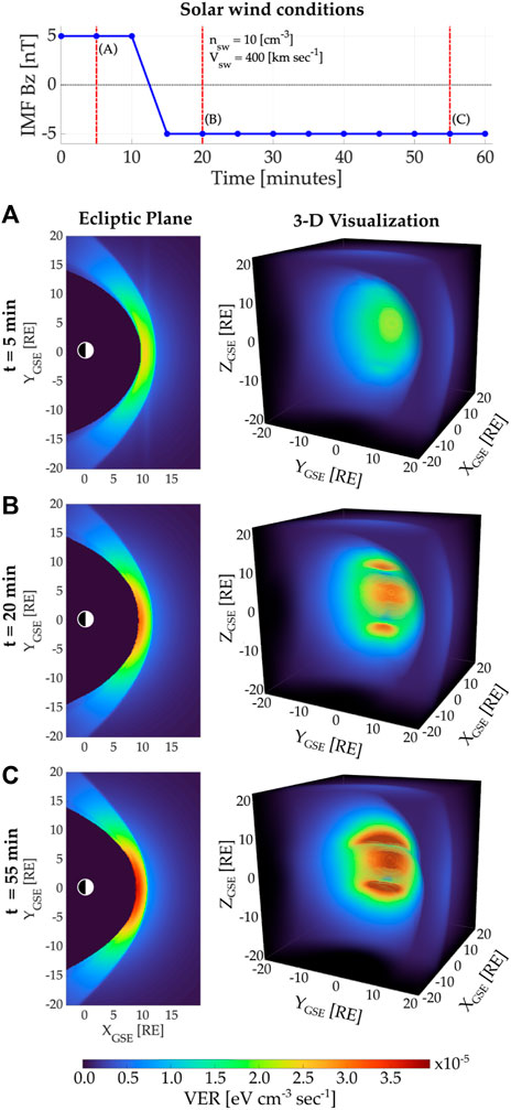
Figure 1. Temporal evolution of magnetosheath soft X-ray emissivities as a response to IMF conditions. The top panel displays IMF Bz values used in this study to simulate the magnetospheric model. The bottom panels show the ecliptic plane and 3-D visualization of the ground truth emissivities for three periods of time: (A) 5 min, (B) 20 min, and (C) 55 min after the start of the simulation.
3.2 Spacecraft mission design
Model-free, time-dependent, and 3-D tomographic reconstructions of soft X-ray emissivities in the magnetospheric region require simultaneous observations from distinct vantage points that can provide sufficient spatial information about the target. In this context, we evaluate tomographic reconstructions using a two-satellite configuration based on the results reported by Jorgensen et al. (2022), which indicate that using two soft X-ray imagers significantly reduces the estimation error obtained with a single instrument. Also, in a realistic scenario, using two satellites would reduce the cost of implementing additional space-based platforms and imaging sensors.
Our design of a spacecraft orbit closely follows that one proposed by Sibeck et al. (2023) for the Solar-Terrestrial Observer for the Response of the Magnetosphere (STORM) mission concept, whose objective is to continuously track and quantify the flow of solar wind energy through the magnetosphere using a set of optical instruments that measure energetic neutral atom (ENA) from the ring current, far ultraviolet (FUV) emission from the auroral region, and soft X-ray emission mainly from the dayside magnetosheath. Our study focused on the analysis of the soft X-ray measurements. The STORM mission concept comprises a single spacecraft in a circular orbit with a radius of 30 RE and an inclination of 90° with respect to the ecliptic plane. The orbit’s orientation is nearly fixed in the inertial frame, allowing the Sun-Earth direction to rotate 360° relative to the orbit over 6 months. The spacecraft is three-axis controlled, with one body axis always to the nadir and the other two axes controlled to keep the sun on one side of the vehicle. Further, the soft X-ray imager onboard the STORM mission has a square field-of-view (FOV) of 23 [deg] and a constant boresight direction canted 18.5 [deg] towards the sun direction in the spacecraft body frame. Aside from periods of low orbital beta angle (Sun near the plane of the orbit), this design allows nearly continuous imaging of the subsolar point at 10 RE (nominal location of the magnetopause).
The objective of this manuscript is to conduct a comparison study of tomographic reconstructions of the dayside magnetosheath from soft X-ray observations acquired by two satellites in STORM-like orbits. For this, we simulated seven (7) spacecraft with different phase angles but similar longitudinal locations that will be arranged in pairs for the tomographic process. Figure 2 shows the distributions of these satellites named spacecraft 0 (SC0) to spacecraft 6 (SC6) along the circular orbit (gray curve). The phase angles between satellites are fixed, and their values (in units of degrees) with respect to SC0 are SC1: 60 [deg], SC2: 75 [deg], SC3: 90 [deg], SC4: 105 [deg], SC5: 120 [deg], and SC6: 180 [deg].
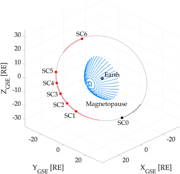
Figure 2. The spacecraft mission has been designed to have a circular orbit (grey solid line) with a radius of 30 RE and an inclination of 90° with respect to the ecliptic plane. The black dot shows the location of spacecraft 0 (SC0), and the red dots show the location of spacecraft one to 6 (SC1 − SC6). Blue dots show an example of a temporally static dayside magnetopause. In this study, we evaluate the feasibility of tomographic estimation of soft X-ray emissivities using ensembles of two spacecraft with SC0 as the reference satellite.
3.3 The impact of orbit selection on tomography feasibility
In this work, we assert that tomographic reconstruction can be performed if and only if the two imaging instruments observe a given target from different vantage points simultaneously. Although this condition is ensured by our design of the imager’s boresight direction that allows nearly continuous observation of the subsolar point at 10 RE, there are periods of time in which one or two imagers point sunward. To avoid contamination from direct sunlight, we define a Sun-Earth avoidance angle equal to 45 [deg]. In other words, if the angle created by the Sun-Earth line (XGSE) and the LOS direction
Based on the previous requirements, Figure 3 shows locations (in GSE spherical coordinates) where tomography is feasible using a pair of spacecraft for a period of 6 months. In each panel, the gray dots indicate the 1-h interval position of the SC0 (at r ≈ 30RE) during a complete translation around Earth. The blue dots show locations where SC0 and SCX (with X ∈ [1, 2, 3, 4, 5, 6]) simultaneously acquire soft X-ray radiance data free from sunlight contamination, i.e., tomography is possible. The number of locations to perform tomography significantly reduces as the phase angle between SC0 and SCX reaches 180 [deg], especially near the low-latitude region, as shown in the bottom right panel (SC0 and SC6). In order to conduct a comparison study of tomographic estimations using these six two-satellite configurations, we selected two vantage points for SC0 where tomography is feasible with all the remaining spacecraft. They are named P1 and P2 and are depicted as red stars in all six panels. Their specific positions in GSE Cartesian coordinates are P1 = [4.846, −14.143, −26.085] RE and P2 = [3.941, 14.679, 25.827] RE.
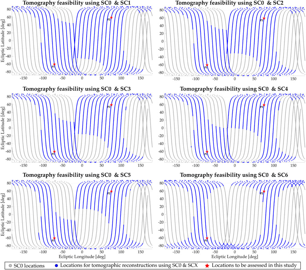
Figure 3. Each panel shows the locations of SC0 during a complete translation of the satellite around Earth (6-month period). The blue dots indicate positions where a tomographic reconstruction of the magnetosheath emissivity is possible using both SC0 and SCX (X ∈{1,2,3,4,5,6}). Gray dots indicate locations where tomography is not feasible since one or both sensors are contaminated by direct sunlight. The red stars (named P1 and P2) indicate vantage points for SC0 where tomographic reconstructions using SC0/SCX data are evaluated in this study.
Figure 4 shows additional analysis for tomographic feasibility using these two-satellite configurations. Each panel shows a histogram of the number of hours when tomography is possible (using SC0 and SCX) with respect to the ecliptic longitude. The histogram dataset has been generated from data shown in Figure 3 that were accumulated along a 10-deg bin in the longitudinal dimension. The total number of hours when tomography can be performed is included on the top left of each panel. In a period of 6 months, tomography can be conducted between 1736 h (using SC0 and SC6) and 2,503 h (using SC0 and SC1). In addition, the number of hours when tomography is feasible remains nearly consistent (at ∼ 110 h) for all six cases when SC0 is located near the terminators (dawn and dusk regions or ecliptic longitudes around ±90 [deg]).
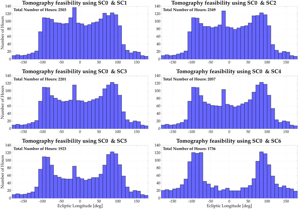
Figure 4. Each panel shows a histogram of the number of hours when tomographic reconstruction is possible using SC0 and SCX (X ∈{1,2,3,4,5,6}) per longitudinal bin (10° widths). The dataset used for each panel corresponds to a complete translation of the satellite around Earth, i.e., a 6-month period.
Furthermore, the total number of hours in a 6-month period is ∼4,320, which indicates that each spacecraft configuration can perform tomography between 40% and 57% of this period. Nevertheless, due to the geometry constraints, continuous acquisition along a longitudinal bin for ∼120 h and covering all latitudes is possible only near the terminators, as shown in Figure 3.
3.4 Four-dimensional tomographic reconstructions of soft X-ray emissivities
In this subsection, we define the experiments needed to evaluate the efficiency of the tomographic results using a two-satellite configuration. Also, we describe the generation of synthetic soft X-ray images and the details of implementing the dynamic tomographic approach.
3.4.1 Experiment settings
We established six experiments with each pair of satellites (SC0/SCX) that include dynamic tomographic reconstructions of the ground truth soft X-ray emissivities from two vantage points (P1 and P2) every 5 min for a 1-h period. Note that the ground truth emissivities (xg) have a 1-min resolution (see specifications in Section 3.1, while our tomographic reconstructions will be performed every 5 min since this is the expected integration time (tint) achieved by the soft X-ray imager (Cucho-Padin et al., 2024).
Figure 5 shows examples of viewing geometry for tomographic reconstruction using a two-satellite configuration. Each row shows the acquisition geometry using the SC0/SCX configuration when the SC0 is at a given vantage point PY (with Y ∈ [1, 2]). The black and red solid lines indicate the imaging sensors’ boresight of SC0 and SCX, respectively. Note that, in all cases, the intersection of boresights occurs near the subsolar point at 10 RE.
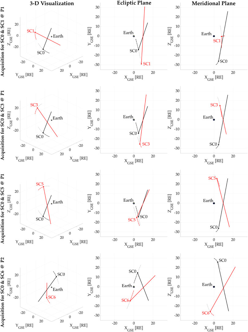
Figure 5. Examples of viewing geometry for tomographic reconstruction of the magnetosheath emissivity. Each row shows the locations (dots) and orbits (curved solid lines) of SC0 and SCX. The solid straight lines represent the boresight of the soft X-ray imagers in the satellites.
3.4.2 Generation of synthetic measurements
To generate synthetic soft X-ray images for each experiment, we first define the pixel resolution of the imaging sensor to be 0.25 × 0.25 [deg2], similar to that specified for NASA’s LEXI experiments in (Cucho-Padin et al., 2024). This value, along with the sensor’s FOV of 23 [deg], yields a 2-D image of 92 × 92 pixels. Next, for each pixel, we calculate its 3-D position and LOS direction
Figure 6 shows an example of a 3-D viewing geometry to generate synthetic soft X-ray measurements. In this case, SC0 is located at vantage point P1, and the SC3 position corresponds to a phase angle of 90 [deg] with respect to SC0. The 3-D soft X-ray emissivities (VER) displayed in the left panel correspond to the start of the simulation (k = 1). The green pyramids represent the sensor FOV of 23 [deg], and the two panels on the right show the synthetic images acquired from each spacecraft. Due to the extension of the FOV, the imaging sensors are able to capture features of the high-altitude cusp (see SC3’s image at coordinates [-10,10] [deg]). For the sake of clarification, these two [92 × 92] pixel images, sorted in a single column vector, form the set of measurements
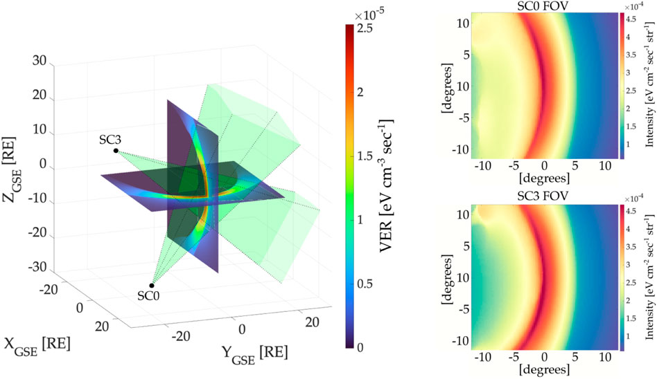
Figure 6. Example of 3-D viewing geometry for tomographic reconstructions of magnetosheath emissivities. In the left panel, the colored slices represent the meridional and ecliptic planes of the soft X-ray volumetric emissivities. The black dots indicate the location of the spacecraft 0 and three at time t =0. The green pyramids represent the instrument FOV, whose interception occurs near the subsolar point at 10 RE. The right panel shows two synthetic 2-D images observed by the SC0 (top sub-panel) and the SC3 (bottom sub-panel) as a result of evaluating Eq. 3 along the pixels’ LOS.
3.4.3 Tomographic inversion process
In this study, we utilized a solution domain that was smaller and had lower spatial resolution than the ground truth rectangular grid, which is more appropriate for this testing stage. For the selection, we considered the following requirements: (i) the volume of this region should include the actual coverage reached by the FOV of both instruments from all vantage points used in the experiments, and (ii) the voxel sizes of this region should secure the correct interpretation of spatial gradients in the soft X-ray emissivity distributions. Thus, our solution domain is a spherical region with the following dimensions in GSE coordinates: radial (r) ∈ [3.75, 20.05] RE, azimuthal (ϕ) ∈ [-110, 100] degrees, and co-latitudinal (θ) ∈ [0, 180] degrees. Also, this region is divided into spherical voxels with sizes Δr = 0.1RE, Δϕ = Δθ = 10 [deg]. The number of voxels per dimension is Nr = 163, Nϕ = 22, and Nθ = 18, and the total number of voxels for this spherical grid is NS = 64, 548. This spherical grid contains most of the soft X-ray emissivities produced on Earth while discarding zones not observed by the optical sensors in the proposed experiments.
We then intersect each pixel’s LOS with the spherical grid to generate the observation matrix
The tomographic reconstructions start at k = 1 and, according to Eq. 10, it requires an estimated vector of emissivities for k − 1,
To generate the covariance matrix of measurements, Rk, we consider that soft X-ray observations, yk, are primarily contaminated by Poisson-distributed shot noise, i.e., yk ∼ Poiss(λ) where λ acts as the mean and variance of the probability distribution. Since the statistical tomography approach introduced in Section 2 establishes that all random vectors involved in the inverse problem should follow a Gaussian probability distribution, we use the approximation
To generate the precision matrix
To explain the spatial structure of σ(r)k−1, we also define the 3-D matrix xk−1(r, ϕ, θ) with size [Nr×Nϕ×Nθ], which is the 3-D spatial rearrangement of elements in vector xk−1. Thus, in Eq. 15, the terms rmin and rmax denote the minimum and maximum radius of the solution domain with values 3.75 and 20.05 RE, respectively. The term
Once all matrices and vectors indicated on the right-hand side of Eq. 10 are provided, we can estimate
3.4.4 Tomographic results
In this section, we present three examples of tomographic reconstructions whose viewing geometry is depicted in the three first rows of Figure 5.
Figure 7 shows the tomographic reconstruction of the magnetosheath soft X-ray emissivities using the SC0/SC1 configuration when the SC0 is located at vantage point P1. Each row shows results corresponding to periods of time: (A) t = 5 min, k = 2, (B) t = 20 min, k = 5, and (C) t = 55 min, k = 12. The first column shows the ecliptic plane of the reconstruction, and the white lines display the boundaries of the spherical grid used as the solution domain. The second column shows a 3-D visualization in GSE Cartesian coordinates. The third column shows plots comparing volumetric emissivities along the Sun-Earth line from 3.75 to 20.05 RE geocentric distance. Here, the blue and red lines show the ground truth and reconstructed emissivities, respectively.
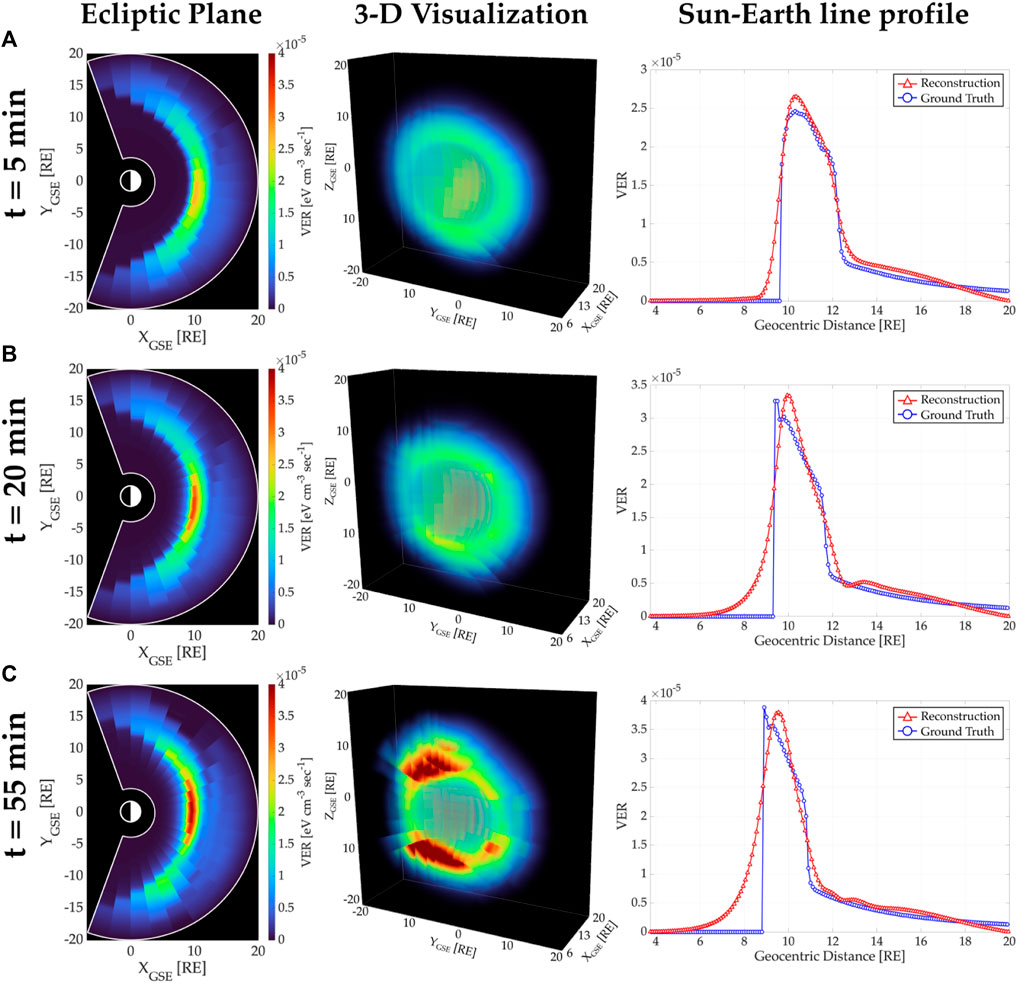
Figure 7. Tomographic reconstruction of the magnetosheath soft X-ray emissivities using the SC0/SC1 configuration when the SC0 is at vantage point P1. Each row corresponds to periods of time: (A) t =5 min, (B) t =20 min, and (C) t =55 min. The first column shows the ecliptic plane of reconstructions, the second column displays a 3-D visualization, and the third column depicts the Sun-Earth line profile of reconstructed and ground truth emissivities.
A visual comparison between our tomographic retrievals of soft X-ray emissivities (in the first column) and the ground truth values (presented in Figure 1) for the same time steps shows the ability of our algorithm to capture the temporal evolution of the magnetosheath density, especially near the Sun-Earth line. The 3-D structure for time step k = 12 (second column, row C) shows that our methodology can reconstruct the dense high-altitude cusps even though the sensors’ FOV does not fully cover them. The structures of reconstructed radial profiles (red lines in the third column) show not only the influence of our assumed exponential standard deviation function σ(r) but also the algorithm’s ability to use observational data to yield expected emissivity spatial distributions. We acknowledge that our methodology cannot reproduce a precise structure of the magnetosheath nor the exact values of VER in the voxels since the reconstruction process is affected by the spherical geometry of our solution domain and its limited extension. Furthermore, the method is unable to yield sharp gradients in the emissivity distributions (as in the blue line), and further investigation should be done to improve the function σ(r) and/or to include a total variation approach (that allows piece-wise reconstruction) within the precision matrix
With an identical format to Figure 7, 8 depicts dynamic tomographic reconstructions of the magnetosheath soft X-ray emissivities using the SC0/SC3 configuration when the SC0 is located at vantage point P1. Although the first column shows a good agreement between reconstructed and ground truth emissivity values and their spatial distributions, there is an evident depletion of emissivities at t = 55 min (row C) starting around noon and propagating towards the dusk region with an increased radial distance. This depletion is also observable in the reconstructed Sun-Earth line profile (red line in the right plot) around 12 RE. On the other hand, the ecliptic plane (left plot) also shows enhancement of emissivities within the magnetosheath near the dawn region (∼[9,-10] RE in the XYGSE plane). In order to analyze these features, we have conducted additional experiments testing several sizes of the solution domain and the voxels. The reader can observe examples of them in our previous published work (Cucho-Padin et al., 2024; 2022) in the context of static soft X-ray and exospheric tomography. Thus, these features are likely related to the usage of a solution domain smaller than the one used to generate the synthetic measurements. This condition imposes a problem in the estimated distribution of volumetric emissivities in those voxels along the measurement LOSs. In tomography, this issue is typically solved when LOSs crossing a given voxel have different angular directions, interconnecting the voxel neighborhood and ultimately providing an adequate distribution of emissivities among them. However, the LOSs from a single sensor are almost parallel, and using two sensors for the reconstructions yields only two distinct LOS directions passing through any voxel in the solution domain. Besides these limitations, the structure of the magnetosheath can be clearly identified, as well as its spatial displacement as a response to the solar wind conditions, which is the aim of this study.
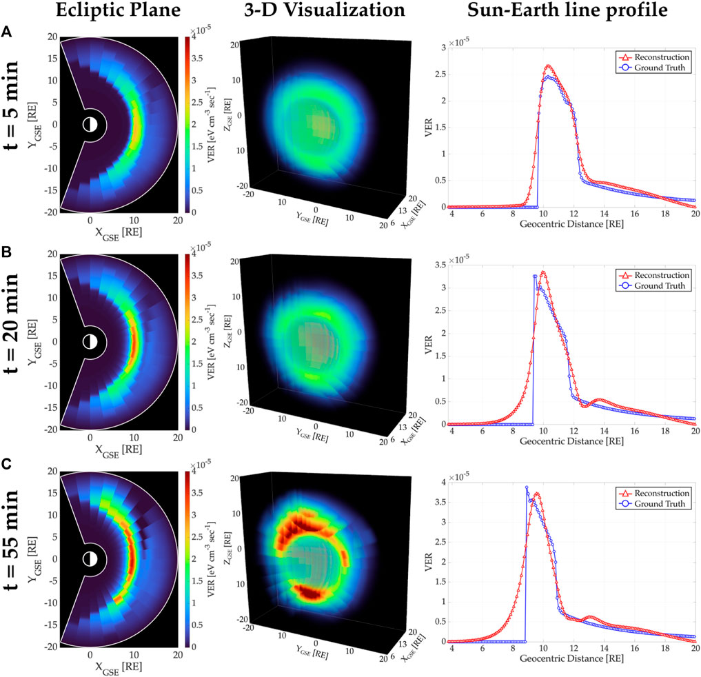
Figure 8. Tomographic reconstruction of the magnetosheath soft X-ray emissivities using the SC0/SC3 configuration when the SC0 is at vantage point P1. Each row corresponds to periods of time: (A) t =5 min, (B) t =20 min, and (C) t =55 min. The first column shows the ecliptic plane of reconstructions, the second column displays a 3-D visualization, and the third column depicts the Sun-Earth line profile of reconstructed and ground truth emissivities.
Figure 9 displays dynamic tomographic reconstructions of the magnetosheath soft X-ray emissivities using the SC0/SC5 configuration when the SC0 is located at vantage point P1. This configuration produces a stronger depletion of emissivities than that one presented in Figure 8 (see row (C). This depletion adversely affects the Sun-Earth line region, as shown in the third column in row (C), around 12 RE geocentric distance. Nevertheless, the emissivity values and their spatial distribution within the magnetosheath still exhibit good agreement with the temporal variation of the ground truth.
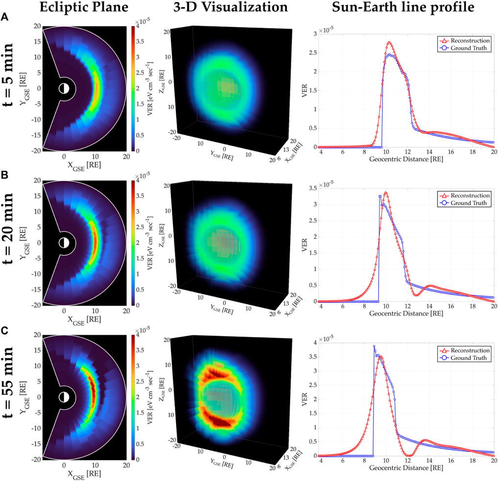
Figure 9. Tomographic reconstruction of the magnetosheath soft X-ray emissivities using the SC0/SC5 configuration when the SC0 is at vantage point P1. Each row corresponds to periods of time: (A) t =5 min, (B) t =20 min, and (C) t =55 min. The first column shows the ecliptic plane of reconstructions, the second column displays a 3-D visualization, and the third column depicts the Sun-Earth line profile of reconstructed and ground truth emissivities.
Another crucial factor affecting the estimation of soft X-ray emissivities is the spatial distribution of LOSs within the solution domain. Figure 10 depicts the LOS density per voxel at the ecliptic plane for the experiments shown in Figures 7–9. In each panel in Figure 10, a colored pixel corresponds to the number of LOSs passing through a spherical voxel in the XYGSE plane. The specific time step for these plots is k = 5, and there is no significant variation in the LOS distributions during the 1-h analysis period. Note that the range of LOS density shown in the color bars differs from panel to panel.
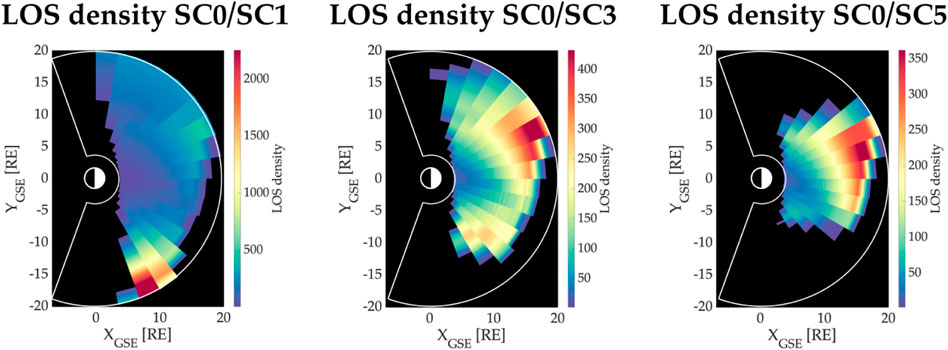
Figure 10. Line-of-sight density per voxels at the ecliptic plane for time step k =5. The colors indicate the number of LOSs passing through each voxel in the ecliptic plane and provide information regarding the spatial distribution of measurements crossing the solution domain.
The region observed by the SC0/SC5 configuration is the smallest among these three experiments owing to its viewing geometry (see the third row in Figure 5). Moreover, these two-satellite observations exhibit a non-uniform distribution with a preference towards radial distances r > 10 RE. The reduced number of observations of the inner magnetospheric region (r < 10 RE) justifies the low efficiency of our algorithm to reconstruct the high gradient structure displayed in the ground truth emissivities (see third column in Figures 7–9).
3.4.5 Assessment of tomographic reconstructions
In order to evaluate our tomographic retrievals of soft X-ray emissivities, we interpolated the resulting values reported in a spherical grid to the high-resolution rectangular grid used for the ground truth. To do so, we used the 3-D interpolation built-in function with the “spline” method in the MATLAB software. Then, we calculated the residual error (Eq. 11) and the Structural Similarity (SSIM) index (Eq. 12) for each reconstruction using definitions provided in Section 2.3. In each panel of Figure 11, the dashed blue line with circular markers and the dotted blue line with square markers show the SSIM values derived from the tomographic reconstructions performed with the SC0/SCX configuration when SC0 is at vantage points P1 and P2, respectively. Similarly, the dashed red line with circular markers and the dotted red line with square markers depict the residual errors obtained from reconstructions at vantage points P1 and P2, respectively.
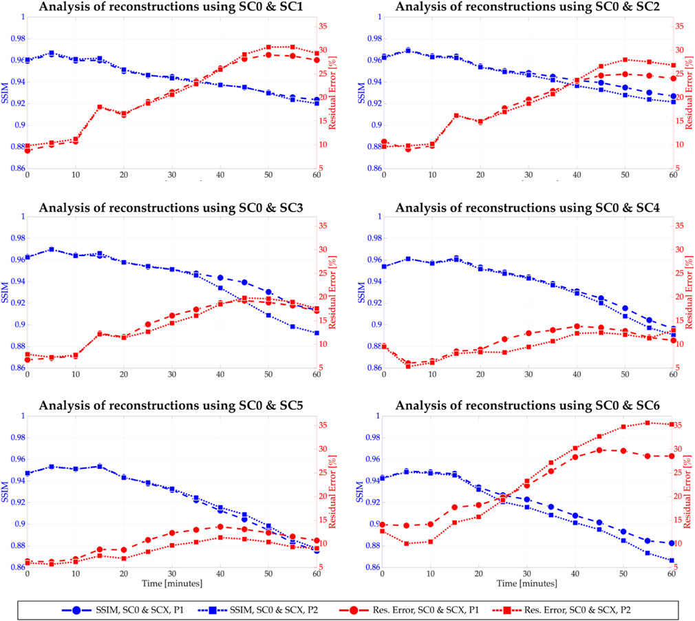
Figure 11. Assessment of tomographic reconstructions. Each panel shows the calculated SSIM and residual error values for the time-dependent tomographic reconstructions. The dashed blue line with circular markers and the dotted blue line with square markers show the SSIM values obtained from the tomographic reconstruction conducted with SC0 and SCX at the vantage points P1 and P2, respectively. Similarly, the dashed red line with circular markers and the dotted red line with square markers show the residual error values calculated from tomographic reconstructions conducted with SC0 and SCX at the vantage points P1 and P2, respectively.
In all panels, the SSIM index shows minimal variation for the first 10 min of the simulation (k ∈ [0, 3]) but shows a monotonically decrease after that period. This feature is highly correlated to the response of the magnetosphere to the sudden change in the Bz component of the IMF. Indeed, the analysis of the MHD simulations reveals a fast Earthward movement of the magnetosheat starting at t = 10 min. In addition, the decreasing trend in the SSIM values is also linked to the displacement of the magnetosheath occurring in less than 5 min, which is our selected reconstruction cadence. Based on the Kalman filtering algorithm used in our approach, each reconstruction depends on current measurements and a previously estimated model that, in our case, was obtained 5 min before. As a result, our tomographic estimations exhibit a spatial delay in the 3-D structure imposed by the previous model.
Table 1 shows the averaged values of SSIM and residual error (eres) for each spacecraft configuration. Specifically, we calculated (i) the total average of the indexes that include the results of the 13 dynamic reconstructions, (ii) the average of the indexes for the almost static period of the magnetosheath, i.e., k ≤ 3, and (iii) the average of the indexes for the period when the magnetosheath moves Earthward, i.e., k > 3. Values in bold font indicate the maximum SSIM and the minimum eres per row, which serves to identify the spacecraft configuration that produces the best tomographic reconstructions in our experiments.
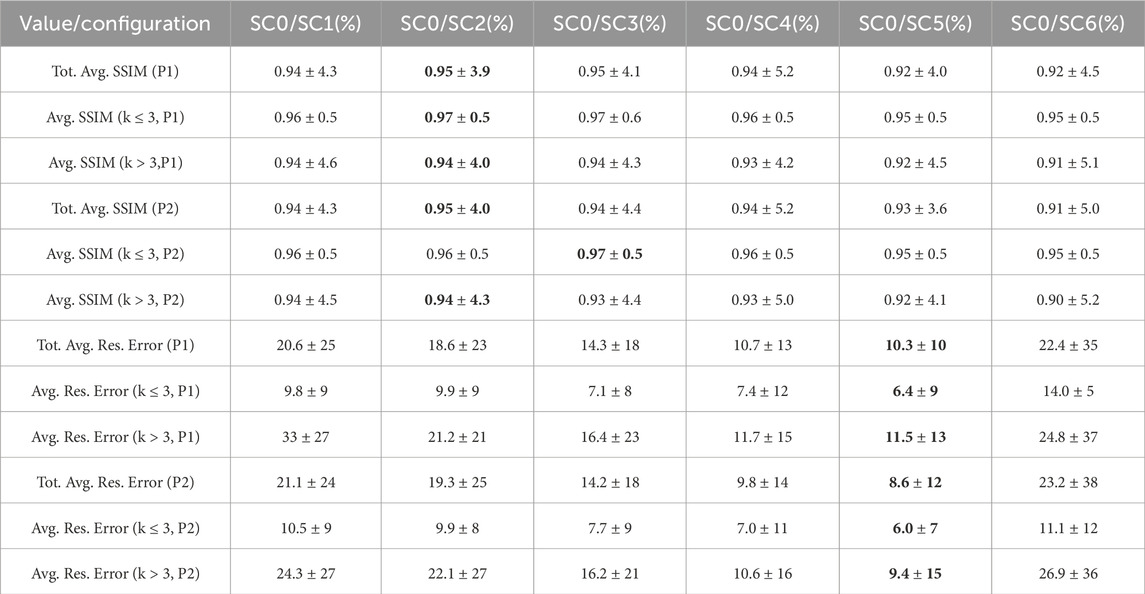
Table 1. Assessment of tomographic reconstruction based on SSIM and residual error values.
3.4.6 Magnetopause location derived from 3-D tomographic reconstructions
In addition, we have calculated the location of the magnetopause (the inner boundary of the magnetosheath) along the Sun-Earth line using the approach presented in (Cucho-Padin et al., 2024), which utilizes a radial profile of reconstructed emissivities and calculates its first derivative along it. The radial position with the highest derivative is considered the current position of the magnetopause (MP). Figure 12 shows the calculation of the MP location (in units of RE) for each dynamic reconstruction. In each panel, the black line with circular markers denotes the ground truth location of the magnetopause extracted from the MHD simulation. The blue line with square markers and the red line with triangular markers indicate the MP radial positions using the SC0/SCX configuration from vantage points P1 and P2, respectively. Since the radial resolution in the spherical grid and the axial resolution in the rectangular grid are identical with value Δr = Δx = 0.1 RE, the error in magnetopause location can only adopt discrete values as in

Figure 12. Magnetopause location derived from tomographic reconstructions. In each panel, the solid black line with circular markers indicates the ground truth magnetopause location derived from the MHD magnetospheric model. The dashed blue line with square markers and the dotted red line with triangular markers indicate the magnetopause location derived from tomographic reconstructions using SC0 and SCX at vantage points P1 and P2, respectively.
An alternative method to quantify the error in the magnetopause location is calculating the average of the error using the formula
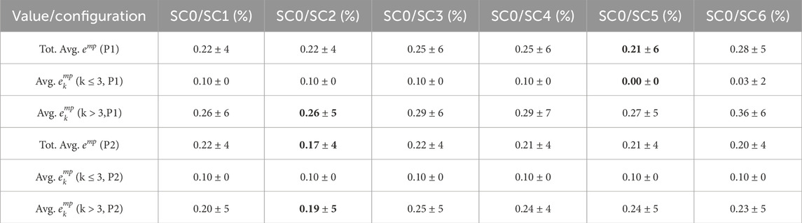
Table 2. Error in the magnetopause location.
4 Discussion and conclusion
This work aims to (i) demonstrate the capability of a statistically-based tomographic approach to reconstruct the time-dependent and 3-D soft X-ray magnetospheric emissivities and (ii) support the design of multi-spacecraft missions that include wide FOV imagers aiming for optical tomography. For this purpose, we simulated the response of the terrestrial magnetosphere to varying solar wind conditions using the MHD OpenGGCM model. The resulting magnetospheric plasma model, along with an assumed neutral exosphere, was used to generate the ground truth emissivities. Then, we designed orbits for a set of two-satellite configurations that can provide simultaneous soft X-ray observations of the dayside magnetosphere. Finally, we used these 2-D images and a dynamic tomographic technique based on Kalman Filtering and Gaussian Markov Random Field theory to reconstruct the 3-D soft X-ray emissivity distributions. In order to determine the spacecraft configuration that achieves the lowest reconstruction error, we calculated the SSIM index and the residual error for each experiment.
In this study, we did not include background soft X-ray contamination nor Poisson-distributed shot noise in the reconstruction process, as our main scope is to introduce the 4-D tomographic technique and a methodology for multi-spacecraft orbit selection based on the tomographic results. Nevertheless, in a realistic scenario, we need to include several sources of uncertainty as those listed below.
1. The image sensor’s responsivity, along with a selected integration time, determines the total number of digital counts to be used in the reconstructions. A low responsivity and/or short integration time would yield a digital image with a low number of counts that can be highly affected by shot noise, thus, precluding the characterization of spatial structures in the observed scene.
2. The point spread function (PSF) of the imaging sensor may induce systematic error in 3-D tomographic retrievals as the PSF distorts object shapes in the scene. An adequate deconvolution algorithm is needed to extract this effect (Schmitz, M. A. et al., 2020).
3. The pointing knowledge determines the accuracy of the spacecraft to point towards a given target. In tomography, an error in the pointing knowledge directly affects the generation of the observation matrix, Lk, as it highly depends on the precision of the LOS directions,
A thorough study of the effect of the listed factors on the tomographic reconstruction of a static magnetosheath is provided in (Cucho-Padin et al., 2024).
Tomographic results displayed in Figures 7–9 present artifacts that are highly related to (i) the use of a smaller solution domain than the one used to generate the measurements (see Section 3.4.4), (ii) the difference between the reconstruction cadence (5 min) and the speed of the magnetosheath Earthward movement, and (iii) the non-uniform distribution of LOSs passing through the solution domain.
In a real scenario, the actual extension of the region with terrestrial soft X-ray emitters is unknown and can deviate from those estimated by MHD models. On the other hand, the solution domain, needed for the tomography approach, requires fixed dimensions that depend on computational resources, such as RAM memory, to allocate vectors and matrices in Eq. 10, and/or the number of cores for the inversion process. Hence, it is likely that the region selected as the solution domain does not cover the entire soft X-ray emission zone. Our study simulates this scenario providing crucial insights about the spatial distribution of retrieved emissivities.
The reconstruction cadence is restricted by the selection of the integration time, which in turn depends on the number of digital counts required in the output image to reduce the effect of the shot noise. In our simulations, the integration time was selected as 5 min because, with this duration, the upcoming LEXI and SMILE missions are expected to capture soft X-ray images with a strong signal-to-noise ratio. The MHD simulations of the magnetosphere exhibited a rapid and Earthward movement of the magnetosheat that was not reproduced accurately using our proposed technique. However, the specific analysis of the magnetopause location at the Sun-Earth line (Section 3.4.6), needed to understand dayside magnetic reconnection dynamics, reveals that our estimations follow the displacement pattern for all experiments as shown in Figure 12. Also, the maximum average error in magnetopause location reported in Table 2 is 0.36 RE.
The LOS distributions within the solution domain displayed in Figure 10 serve to identify covered regions where tomography reconstruction is more effective. The black pixels are regions not observed by both sensors, and their estimations will highly depend on the previous model,
Although the experiments reported in this study are based on a single dynamic MHD model of the magnetosphere, we can still infer that our technique is robust enough to reconstruct soft X-ray emissivities corresponding to an MHD model whose input solar wind parameters produce (1) at most an Earthward displacement of 0.2 Re/minute of the magnetopause location, and (2) sufficient soft-X ray emitters to handle an appropriate signal to noise ratio. The latter is specifically related to the solar wind density and should be large enough to produce a soft X-ray intensity greater than 1 [eV/cm2/sec/str] along a pixel line-of-sight (see Figure 6) under the assumption of zero noise. The two abovementioned constraints allow us to generate an extensive combination of input solar wind conditions in which our tomography methodology is efficient.
In this study, we have used the methodology provided by Samsonov et al. (2022) to extract the inner magnetospheric region of the MHD model since solar wind ions would not populate this zone and would not create soft X-ray emitters. Nevertheless, the sudden depletion of soft X-ray emissivities to zero values in the inner magnetosphere (see Figure 1) is likely to be an artifact of this method. A more sophisticated analysis for inner magnetospheric extraction has been used in (Sibeck et al., 2018) (see Figure 58, left panel) and displays a gradual variation of soft X-ray emitters in the same region. Therefore, our dynamic tomography approach, which essentially supports this progressive change in the emissivity (the first component of Eq. (15)), might provide better results under a more realistic scenario.
Our study presented a quantitative comparison of reconstruction errors for each experiment. This has been conducted using the SSIM index and the residual error of the estimated emissivities. According to Table 1, the highest SSIM values are achieved by the SC0/SC2 configuration, and the lowest residual errors are yielded when the SC0/SC5 configuration is used. Additionally, we quantified the error in magnetopause location, whose detection is one of the main goals of estimating the 3-D structure of emissivities. According to Table 2, the lowest averaged error in MP location is achieved by the SC0/SC5 configuration. Also, the lowest averaged error in MP location during the dynamic stage of the magnetosphere is obtained when the SC0/SC2 configuration is used. Other factors to be considered in the selection of the best spacecraft configuration for soft X-ray tomography are (1) the total number of hours in a 6-month period in which tomography is possible (see Figure 3) and (2) the coverage of LOS within the solution domain (displayed in Figure 10 for the SC0/SC5 case). Hence, the configuration SC0/SC2 has ∼22% more hours to perform tomography in a 6-month period than SC0/SC5. Similarly, the SC0/SC2 configuration enables the two imaging sensors to cover ∼32% more 3-D voxels (in the solution domain) than SC0/SC5. In sum, we found that the configuration SC0/SC2, with phase angle 75 [deg], is the best configuration among the seven presented in this study to provide a low error in the tomographic reconstruction of soft X-ray emissivities, a low error in detecting the magnetopause location, and a large number of hours during a 6-month period to perform tomography.
Finally, we evaluate our tomography methodology for the selected SC0/SC2 configuration over the 6-month period orbit. To do so, we have divided the spherical shell with radius 30 RE, where the spacecraft transits, into 20 ° × 20 ° pixels and perform the 60-min dynamic tomographic reconstruction for the SC0’s location that is closest to the center of a given pixel. In Figure 13, we report the average values (k ∈ [1, 13]) for the SSIM index, residual error in the reconstructions, and error in the magnetopause location. High values of SSIM indexes and low values of the residual errors in reconstructions are mainly located near the terminators at any latitude. These results agree with static reconstructions reported in (Cucho-Padin et al., 2024), wherein the best SSIM was obtained from tomographic reconstructions of the magnetosheath that have the sensor’s line-of-sight almost perpendicular to the Sun-Earth line. On the other hand, we note that estimation in the magnetopause location is also better in the terminators, with a preference toward the dusk region. Since our MHD simulations only account for changes in the Bz component of the IMF, it is not expected to have significant asymmetries in the soft X-ray emissivities along the longitudes; therefore, this effect is likely linked to the acquisition geometry which is not entirely symmetric for conjugate longitudes.
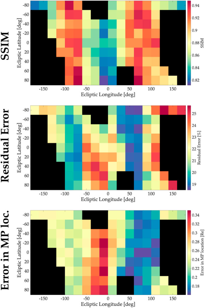
Figure 13. Average values of SSIM, residual errors in reconstructions, and errors in magnetopause location for the SC0/SC2 configuration during a 6-month period.
Data availability statement
The raw data supporting the conclusion of this article will be made available by the authors, without undue reservation.
Author contributions
GC-P: Conceptualization, Formal Analysis, Investigation, Methodology, Software, Visualization, Writing–original draft, Writing–review and editing. HC: Data curation, Methodology, Supervision, Writing–review and editing, Investigation. JJ: Data curation, Writing–review and editing, Investigation, Methodology. MS: Data curation, Writing–review and editing. KM: Methodology, Supervision, Writing–review and editing. DS: Methodology, Supervision, Writing–review and editing, Funding acquisition. JN: Formal Analysis, Supervision, Validation, Writing–review and editing. EV: Formal Analysis, Methodology, Validation, Writing–review and editing.
Funding
The author(s) declare financial support was received for the research, authorship, and/or publication of this article. This work was supported by NASA’s HUSPI program, and the NASA Goddard Space Flight Center through Cooperative Agreement 80NSSC21M0180 to Catholic University, Partnership for Heliophysics and Space Environment Research (PHaSER). Hyunju Connor gratefully acknowledges the NASA grant (80MSFC20C0019).
Conflict of interest
The authors declare that the research was conducted in the absence of any commercial or financial relationships that could be construed as a potential conflict of interest.
Publisher’s note
All claims expressed in this article are solely those of the authors and do not necessarily represent those of their affiliated organizations, or those of the publisher, the editors and the reviewers. Any product that may be evaluated in this article, or claim that may be made by its manufacturer, is not guaranteed or endorsed by the publisher.
References
Aubry, M. P., Russell, C. T., and Kivelson, M. G. (1970). Inward motion of the magnetopause before a substorm. J. Geophys. Res. (1896-1977) 75, 7018–7031. doi:10.1029/JA075i034p07018
Branduardi-Raymont, G., Wang, C., Escoubet, C. P., Adamovic, M., Agnolon, D., Berthomier, M., et al. (2018). Smile definition study report (red book).
Butala, M. D., Hewett, R. J., Frazin, R. A., and Kamalabadi, F. (2010). Dynamic three-dimensional tomography of the solar corona. Sol. Phys. 262, 495–509. doi:10.1007/s11207-010-9536-1
Collier, M. R., and Connor, H. K. (2018). Magnetopause surface reconstruction from tangent vector observations. J. Geophys. Res. Space Phys. 123 (10), 189–210. doi:10.1029/2018JA025763
Connor, H. K., and Carter, J. A. (2019). Exospheric neutral hydrogen density at the nominal 10 R<i>E</i> subsolar point deduced from xmm-Newton X-ray observations. J. Geophys. Res. Space Phys. 124, 1612–1624. doi:10.1029/2018JA026187
Connor, H. K., Sibeck, D. G., Collier, M. R., Baliukin, I. I., Branduardi-Raymont, G., Brandt, P. C., et al. (2021). Soft x-ray and ena imaging of the earth’s dayside magnetosphere. J. Geophys. Res. Space Phys. 126, e2020JA028816. doi:10.1029/2020JA028816
Cucho-Padin, G., Connor, H., Jung, J., Walsh, B., and Sibeck, D. G. (2024). Finding the magnetopause location using soft x-ray observations and a statistical inverse method. Earth Planet. Phys. 8, 184–203. doi:10.26464/epp2023070
Cucho-Padin, G., Kameda, S., and Sibeck, D. G. (2022). The earth’s outer exospheric density distributions derived from procyon/laica uv observations. J. Geophys. Res. Space Phys. 127, e2021JA030211. doi:10.1029/2021JA030211
Dungey, J. W. (1961). Interplanetary magnetic field and the auroral zones. Phys. Rev. Lett. 6, 47–48. doi:10.1103/PhysRevLett.6.47
Feller, W. (1968). An introduction to probability theory and its applications. New York, USA: Wiley.
Jansen, F., Lumb, D., Altieri, B., Clavel, J., Ehle, M., Erd, C., et al. (2001). Xmm-Newton observatory* - i. the spacecraft and operations. A&A 365, L1–L6. doi:10.1051/0004-6361:20000036
Jelínek, K., Němeček, Z., and Šafránková, J. (2012). A new approach to magnetopause and bow shock modeling based on automated region identification. J. Geophys. Res. Space Phys. 117. doi:10.1029/2011JA017252
Jorgensen, A. M., Sun, T., Wang, C., Dai, L., Sembay, S., Wei, F., et al. (2019b). Boundary detection in three dimensions with application to the smile mission: the effect of photon noise. J. Geophys. Res. Space Phys. 124, 4365–4383. doi:10.1029/2018JA025919
Jorgensen, A. M., Sun, T., Wang, C., Dai, L., Sembay, S., Zheng, J., et al. (2019a). Boundary detection in three dimensions with application to the smile mission: the effect of model-fitting noise. J. Geophys. Res. Space Phys. 124, 4341–4355. doi:10.1029/2018JA026124
Jorgensen, A. M., Xu, R., Sun, T., Huang, Y., Li, L., Dai, L., et al. (2022). A theoretical study of the tomographic reconstruction of magnetosheath x-ray emissions. J. Geophys. Res. Space Phys. 127, e2021JA029948. doi:10.1029/2021JA029948
Jung, J., Connor, H. K., Carter, J. A., Koutroumpa, D., Pagani, C., and Kuntz, K. D. (2022). Solar minimum exospheric neutral density near the subsolar magnetopause estimated from the xmm soft x-ray observations on 12 november 2008. J. Geophys. Res. Space Phys. 127, e2021JA029676. doi:10.1029/2021JA029676
Kim, H., Connor, H. K., Jung, J., Walsh, B. M., Sibeck, D., Kuntz, K. D., et al. (2024). Estimating the subsolar magnetopause position from soft x-ray images using a low-pass image filter. Earth Planet. Phys. 8, 1–11. doi:10.26464/epp2023069
Koga, D., Gonzalez, W. D., Souza, V. M., Cardoso, F. R., Wang, C., and Liu, Z. K. (2019). Dayside magnetopause reconnection: its dependence on solar wind and magnetosheath conditions. J. Geophys. Res. Space Phys. 124, 8778–8787. doi:10.1029/2019JA026889
Kuntz, K. D., Collado-Vega, Y. M., Collier, M. R., Connor, H. K., Cravens, T. E., Koutroumpa, D., et al. (2015). The solar wind charge-exchange production factor for hydrogen. Astrophysical J. 808, 143. doi:10.1088/0004-637X/808/2/143
Norberg, J., Käki, S., Roininen, L., Mielich, J., and Virtanen, I. I. (2023). Model-free approach for regional ionospheric multi-instrument imaging. J. Geophys. Res. Space Phys. 128, e2022JA030794. doi:10.1029/2022JA030794
Norberg, J., Vierinen, J., Roininen, L., Orispää, M., Kauristie, K., Rideout, W. C., et al. (2018). Gaussian markov random field priors in ionospheric 3-d multi-instrument tomography. IEEE Trans. Geoscience Remote Sens. 56, 7009–7021. doi:10.1109/TGRS.2018.2847026
Robertson, I. P., and Cravens, T. E. (2003). X-ray emission from the terrestrial magnetosheath. Geophys. Res. Lett. 30. doi:10.1029/2002GL016740
Samsonov, A., Carter, J. A., Read, A., Sembay, S., Branduardi-Raymont, G., Sibeck, D., et al. (2022). Finding magnetopause standoff distance using a soft x-ray imager: 1. magnetospheric masking. J. Geophys. Res. Space Phys. 127, e2022JA030848. doi:10.1029/2022JA030848
Schmitz, M. A., Starck, J.-L., Ngole Mboula, F., Auricchio, N., Brinchmann, J., Vito Capobianco, R. I., et al. (2020). Euclid: nonparametric point spread function field recovery through interpolation on a graph laplacian. Astronomy Astrophysics 636, A78. doi:10.1051/0004-6361/201936094
Shue, J.-H., Song, P., Russell, C. T., Steinberg, J. T., Chao, J. K., Zastenker, G., et al. (1998). Magnetopause location under extreme solar wind conditions. J. Geophys. Res. Space Phys. 103, 17691–17700. doi:10.1029/98JA01103
Sibeck, D. G., Allen, R., Aryan, H., Bodewits, D., Brandt, P., Brown, G., et al. (2018). Imaging plasma density structures in the soft x-rays generated by solar wind charge exchange with neutrals. Space Sci. Rev. 214, 79. doi:10.1007/s11214-018-0504-7
Sibeck, D. G., Murphy, K. R., Porter, F. S., Connor, H. K., Walsh, B. M., Kuntz, K. D., et al. (2023). Quantifying the global solar wind-magnetosphere interaction with the solar-terrestrial observer for the response of the magnetosphere (storm) mission concept. Front. Astronomy Space Sci. 10. doi:10.3389/fspas.2023.1138616
Walsh, B. M., Collier, M. R., Kuntz, K. D., Porter, F. S., Sibeck, D. G., Snowden, S. L., et al. (2016). Wide field-of-view soft x-ray imaging for solar wind-magnetosphere interactions. J. Geophys. Res. Space Phys. 121, 3353–3361. doi:10.1002/2016JA022348
Walsh, B. M., Kuntz, K. D., Busk, S., Cameron, T., Chornay, D., Chuchra, A., et al. (Forthcoming 2024). The lunar environment heliophysics x-ray imager (lexi) mission. Space Sci. Rev.
Wang, R. C., Li, D., Sun, T., Peng, X., Yang, Z., and Wang, J. Q. (2023). A 3d magnetospheric ct reconstruction method based on 3d gan and supplementary limited-angle 2d soft x-ray images. J. Geophys. Res. Space Phys. 128, e2022JA030424. doi:10.1029/2022JA030424
Weisskopf, M. (2003). The chandra x-ray observatory: an overview. Adv. Space Res. 32, 2005–2011. doi:10.1016/S0273-1177(03)90639-9
Whittaker, I. C., and Sembay, S. (2016). A comparison of empirical and experimental o7+, o8+, and o/h values, with applications to terrestrial solar wind charge exchange. Geophys. Res. Lett. 43, 7328–7337. doi:10.1002/2016GL069914
Keywords: 3-D/4-D tomography, soft X-Ray, magnetosheath, multi-spacecraft measurements, optical remote sensing
Citation: Cucho-Padin G, Connor H, Jung J, Shoemaker M, Murphy K, Sibeck D, Norberg J and Rojas E (2024) A feasibility study of 4-D tomography of soft X-ray magnetosheath emissivities using multi-spacecraft measurements. Front. Astron. Space Sci. 11:1379321. doi: 10.3389/fspas.2024.1379321
Received: 31 January 2024; Accepted: 16 April 2024;
Published: 06 May 2024.
Edited by:
Thomas Earle Moore, Third Rock Research, United StatesReviewed by:
Bertrand Bonfond, University of Liège, BelgiumJim Burch, Southwest Research Institute (SwRI), United States
Ruth Skoug, Los Alamos National Laboratory (DOE), United States
Copyright © 2024 Cucho-Padin, Connor, Jung, Shoemaker, Murphy, Sibeck, Norberg and Rojas. This is an open-access article distributed under the terms of the Creative Commons Attribution License (CC BY). The use, distribution or reproduction in other forums is permitted, provided the original author(s) and the copyright owner(s) are credited and that the original publication in this journal is cited, in accordance with accepted academic practice. No use, distribution or reproduction is permitted which does not comply with these terms.
*Correspondence: Gonzalo Cucho-Padin, Z29uemFsb2F1Z3VzdG8uY3VjaG9wYWRpbkBuYXNhLmdvdg==