The electron density at the midpoint of the plasmapause

The high density plasmasphere in the magnetosphere is often separated from a lower density region outside of the plasmasphere, called the plasmatrough, by a sharp gradient in electron density called the plasmapause. Here we use plasmapause events identified from electron density data from the ISEE, CRRES, Polar, and IMAGE missions, and the nonlinear genetic algorithm TuringBot, to find models for the electron density at the midpoint of the plasmapause, n_e,pp. A good model for n_e,pp should include dependence on L, which is the strongest dependence. But models can be improved by including weaker dependencies on the magnetic local time, MLT, the solar EUV index F10.7, and geomagnetic activity as indicated by averages of Kp and AE. The most complicated model that we present predicts n_e,pp within a factor of 1.64, and is within the range of observed plasmapause densities for about 96% of our events. These models can be useful for separating plasma populations into plasmasphere-like and plasmatrough-like populations. We also make available our database of electron density measurements categorized into various populations.

1 Introduction

The plasmapause, as originally defined, is a steep gradient in electron density separating the region of relatively high density close to the earth, called the plasmasphere, from the region of depleted density beyond, called the plasmatrough (Carpenter and Anderson, 1992). It has long been known that the density in both the plasmasphere and plasmatrough steeply decreases with respect to L. Then, the density at the midpoint of the plasmapause, n_e,pp, must also decrease steeply with respect to L. Indeed, an adequate model for n_e,pp could be found by taking the logarithmic mean between the electron density from the plasmasphere and plasmatrough models.

For the purposes of this paper, L is defined as the maximum radius to any point on a magnetospheric magnetic field line using the TS05 magnetic field model (Tsyganenko and Sitnov, 2005), R_max,TS05, divided by the radius of the earth, R_E.

This paper has two modest goals: first, to point out clearly that a model for n_e,pp, which can be used to separate plasmasphere and plasmatrough populations, should be L-dependent, and second, to show that simple models can suffice to separate those populations in most cases.

Though it is notoriously difficult to model the position of the plasmapause, it turns out that it is much easier to model the density at the midpoint of the plasmapause, given its position in space. Sheeley et al. (2001) suggested a simple formula for the separation of plasmasphere-like and plasmatrough-like plasma as follows:

$n_{\text{e,pp}}=10{\left(6.6/L\right)}^4{\mathrm{c}\mathrm{m}}^{-3},(1)$

(see Eq. (5) in their study) (where a misprint in the power “4” has been corrected). Although this dependence is reasonable, no evidence was presented that this formula was optimal.

Denton et al. (2004) stated that the following slight modification seemed to work better for distinguishing plasmasphere and plasmatrough plasma:

$n_{\text{e,pp}}=15{\left(6.6/L\right)}^4{\mathrm{c}\mathrm{m}}^{-3},(2)$

but again, they did not offer any evidence that this was the case.

In addition to finding models for n_e,pp in order to provide a boundary value for the electron density between that of the plasmasphere and that of the plasmatrough, we will also use this opportunity to make public our magnetospheric electron density datasets, which should be useful for other studies.

Our data are described in Section 2, and the results are presented in Section 3. Discussion follows in Section 4.

2 Data and methods

2.1 Missions and density values

We used electron density measurements from four spacecraft, namely, the International Sun-Earth Explorer 1 (ISEE-1), the Combined Release and Radiation Effects Satellite (CRRES), Polar, and the Imager for Magnetopause-to-Aurora Global Exploration (IMAGE) spacecraft.

Table 1 shows the spacecraft specifications, including the spacecraft orbits and the years and phases of the solar cycle when the electron density measurements were made. The selection of data has good coverage of spatial locations within the inner magnetosphere and different conditions over the solar cycle. Using nonlinear regression (Section 2.3), which takes into account separate dependencies independently, it is possible to combine these measurements to determine the characteristics of the plasmapause density for a variety of conditions (when combining data from different spacecraft, realistic results are not always obtained using simple binning, as demonstrated by Denton et al. (2022)). For instance, some of our formulas depend on the solar EUV index F10.7, which varies with the solar cycle.

Table 1

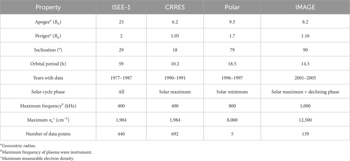
Table 1. Spacecraft specifications.

All electron density measurements were found from plasma wave measurements, either using the upper hybrid resonance frequency or the lower edge of the continuum frequency within the plasmatrough (LeDocq et al., 1994; Gurnett et al., 1995; Carpenter et al., 2000; Denton et al., 2012). Typical errors in electron density might be roughly 20% (Denton et al., 2022).

The plasma wave instruments used were the Plasma Wave Investigation on ISEE (Gurnett et al., 1979), the Plasma Wave Experiment on CRRES (Anderson et al., 1992), the Plasma Wave Instrument on Polar (Gurnett et al., 1995), and the passive radio data from the Radio Plasma Imager Investigation on IMAGE (Reinisch et al., 2000). Because the electron density is proportional to the square of the plasma frequency, the highest possible electron density that can be measured by one of these instruments is determined by the upper limit of the frequency. The maximum frequency and maximum electron density values are listed for each spacecraft in Table 1. The lowest upper limit of frequency is for ISEE and CRRES, which could measure electron density only up to 1984 cm⁻³ (this explains the cutoff in measurements that is discussed in Section 3.1).

2.2 Categorization of plasma regions including the plasmapause

The categorization of data points by region was performed manually using a computer program that generated plots like Figure 1, using data from ISEE observed on 10 November 1997, between 1800 and 2400 UT. The groupings of data points were selected by dragging the mouse over a selection of points. Figure 1 shows data points in the plasmasphere, plasmapause, plasmatrough, and magnetosheath. The slope of the plasmapause was defined using the outermost data point in the plasmasphere and the innermost data point of the plasmatrough, and was required to be at least a factor of 3 within a change in L of 0.4. This corresponds to a slightly smaller slope than that required by Carpenter and Anderson (1992), a factor of 5 within a change in L of 0.5. We used the smaller slope criterion because there were many events for which there was clearly a plasmapause, but the slope was not quite as large as that required by Carpenter and Anderson (1992).

In our database, a plasmapause was defined as a drop in density of at least a factor of 3, but for this study, we use only a subset of the plasmapause observations with a drop in density of a factor of 5. Data points within the plasmapause were within the largest region with the required slope, as shown in Figure 1.

When there was more than one region of L with the required slope, only the one at the lowest L was considered to be the plasmapause for the purpose of this study.

Note that a steep gradient identifying the plasmapause is not always observed, as noted by Denton et al. (2004). This situation can occur when plasmaspheric refilling has occurred for a long enough time so that the entire magnetosphere has density at plasmaspheric levels or when a spacecraft passes radially through a plasmaspheric plume (normally on the dayside). However, the dataset used here only includes those observations for which a plasmapause is observed.

In addition to the condition on the slope, some other conditions were required. For the polar orbiting spacecraft, namely, Polar and IMAGE, only the high-altitude part of the orbit with a geocentric radial distance greater than the minimum L shell sampled by the orbit was used. This criterion was imposed because a plasmapause is not as evident at low altitude and to avoid errors in mapping from low-altitude positions to the equator to determine the L shell.

In order to sample the region of space that is usually within the magnetopause, we limited the L value of the midpoint of the plasmapause, L_pp, to values $\le 10$, and because of the instrumental limitations discussed below, we also required L_pp ≥ 3.25.

The plasmapause was required to extend over no greater a range in L (from the outermost plasmasphere data point to the innermost plasmatrough data point) than 2, and no greater a range in MLT than 2.5 in order to exclude observations with large data gaps. The slope dL/dR_MLT, where dL is a change in L and dR_MLT = (dMLT)(2 pi L/24) is roughly the change in the distance around the Earth due to a change in MLT of dMLT, was also required to be at least $\tan \left(10°\right)=0.176$ to reduce the probability of confusing azimuthal structure with that in the radial direction.

Because we found that some formulas depended on the Auroral Electrojet Index AE, we also required that the quality factor for the averaged measurements of AE (defined below) be at least 1, using quality factors analogous to those described by Qin et al. (2007) (basically, a quality factor of 1 means that the observed quantities may be interpolated, but that they need to be within a correlation time of the observed measurements).

With these conditions, we identified 1,276 plasmapause segments, 440 from ISEE, 692 from CRRES, 5 from Polar, and 139 from IMAGE. The CRRES data (at solar maximum) are overrepresented considering the time span of the mission, but our formulas do take into account the geomagnetic activity, so we hope that this will ameliorate that problem.

Figure 2 shows the equatorial distribution of plasmapause segments (between the outermost plasmasphere data point and the innermost plasmatrough data point) in the solar magnetospheric (SM) or dipole equatorial plane. There is a good distribution at all MLT values between L = 3.25 and about L = 8.5.

For the purpose of developing models, the position of the plasmapause was defined as the position of the spacecraft at the midpoint between the outermost plasmasphere data point (data point at the beginning of the steep slope) and the innermost plasmatrough data point (data point at the end of the steep slope), and the electron density at the midpoint of the plasmapause, n_e,pp, was defined as the logarithmic mean of the outermost plasmasphere and innermost plasmatrough density values (see Figure 1).

Other categories of plasma were also defined, as described in the supplementary information. However, the categories described above are sufficient to define the plasmapause for this paper.

Figure 1

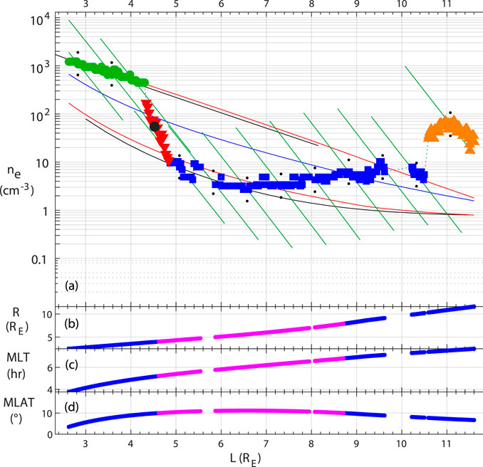
Figure 1. Example of plasma categorization using data from ISEE on 10 November 1997 between 1800 and 2400 UT. (A)Electron density, n_e; (B)geocentric radius R; (C)magnetic local time, MLT; and (D)magnetic latitude, MLAT, plotted versus L≡ R_max,TS05/R_E. Before categorization, the data points appear as in panels b−d, with pink pluses for MLAT$>10°$ and blue pluses for MLAT$\le 10°$. The identified regions are the plasmasphere (green circles), plasmapause (red triangles), plasmatrough (blue squares), and magnetosheath (orange triangles). The upper and lower red and black curves are plasmasphere and plasmatrough curves based on the equations of Carpenter and Anderson (1992), with the red curves adjusted to account for off-equatorial MLAT. The middle blue curve is Eq. 2 with an adjustment to account for MLAT, and the diagonal green line segments have the slope required to identify a plasmapause discussed in the text (the little black dots mark the center of these line segments and can be ignored). The big black circle is the midpoint plasmapause density predicted from model 14 in Table 2.

2.3 Eureqa and TuringBot programs

In order to model the density at the midpoint of the plasmapause, n_e,pp, we did some preliminary analysis using the Eureqa nonlinear genetic regression program (Schmidt and Lipson, 2009), a proprietary product owned by the DataRobot Inc. company, in a manner similar to that of Denton et al. (2022). However, because of changes in DataRobot Inc.’s pricing structure, we switched to the TuringBot program, which functions similarly; the final formulas that we presented were found using TuringBot (see the Data Availability Statement for links to these software programs).

Both of these programs are nonlinear genetic algorithms that find models using analytical formulas. They search the space of possible formulas, spending more time searching for types of formulas that yield less error. Both programs determine a set of formulas of varying complexity. Our TuringBot runs sampled billions of different formulas, and the best-fitting model for each level of complexity was determined using cross-validation with five groups of randomly sorted data. The TuringBot complexity is described by the mathematical operations: a cost of 1 for introducing a variable or constant or calculating a sum, difference, or product; a cost of 2 for division; and a cost of 4 for all other operations, including logarithms and power laws.

Our modeling of n_e,pp proceeded through several iterations in which we examined the dependence of n_e,pp on a number of different parameters: position; phase of the year; geomagnetic indices like the planetary K index (Kp), The disturbance storm time index (Dst), and AE; solar wind parameters like components of the interplanetary magnetic field (IMF), B_Y and B_Z, the solar wind density, solar wind velocity, V, and solar wind dynamic pressure, Pdyn; the F10.7 index measuring solar radiation at 10.7 cm wavelength; the solar wind convection electric field defined by VB_s, where B_s = −B_Z if B_Z < 0 and B_s = 0 otherwise; and the coupling function of Newell et al. (2007), dΦ_MP/dt.

By far, the strongest dependence that we found was on the L value at the midpoint of the plasmapause, L_pp, but some of our models had a dependence on the magnetic local time, MLT, at the midpoint of the plasmapause, MLT_pp, and some geomagnetic indices. From our early runs using Eureqa, we found that a minimum in n_e,pp with respect to MLT occurred at MLT = 3.43 h. For the final modeling runs using TuringBot, we searched for dependence on L_pp, cos (2π(MLT −3.43)/24), sin (2π(MLT −3.43)/24), cos (4π(MLT −3.43)/24), sin (4π(MLT −3.43)/24), F10.7, Dst, and averages of Kp and AE over the previous 3, 6, 12, 24, 48, 96, and 192 h. Terms averaging up to 96 h appeared in the final models. The TuringBot runs searched for the lowest root mean squared (RMS) error of the difference between the observed and modeled log₁₀ (n_e,pp).

3 Results

Figure 3 shows a histogram of the base 10 logarithm of n_e at the outermost data point in the plasmasphere (Figure 3A), at the midpoint of the plasmapause (Figure 3B), and at the innermost data point in the plasmatrough (Figure 3C), as defined in Section 2. There is a two-order-of-magnitude variation in the midpoint density values in Figures 3A,B and a three-order-of-magnitude variation between the lowest plasmatrough density values in Figure 3C and the highest plasmasphere density values in Figure 3A.

Figure 2

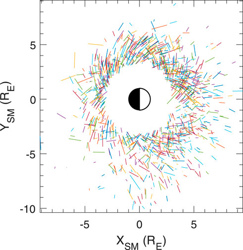
Figure 2. Plasmapause segments (with random colors) from the outermost data point in the plasmasphere to the innermost data point in the plasmatrough in the SM equatorial plane, where X_SM = −L cos (2πMLT/24) and Y_SM = −L sin (2πMLT/24).

Figure 3

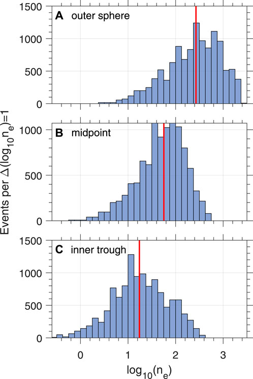
Figure 3. Histogram of electron density values at (A) the outermost point of the plasmasphere, (B) the midpoint of the plasmapause, and (C) the innermost point of the plasmatrough. The red vertical line on each panel is the median value, 57.4 cm⁻³ for panel (B).

The median plasmapause density for our data with no lower limit on L_pp was 69.5 cm⁻³ or 56.7 cm⁻³ for L_pp ≥ 3.25 (marked by the vertical red line in Figure 3B).

3.1 L dependence of the density at the midpoint of the plasmapause

In Figure 4, line segments are drawn from the density of the outermost plasmasphere data point to that of the innermost plasmatrough data point versus L. There is a rough upper boundary for the high-density data points and a rougher lower boundary for the low-density data points. There is a steep L dependence for the density values within the plasmapause.

Figure 4

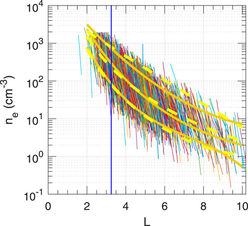
Figure 4. Plasmapause segments (with random colors) versus L. The three solid gold curves are (highest) a fit to the density of the outermost data points in the plasmasphere, Eq. 3; (middle) a model for the midpoint plasmapause density, Eq. 5; and (lowest) a fit to the innermost data points in the plasmatrough, Eq. 4. The three dashed yellow curves are (highest) a curve derived from the plasmasphere density model of Carpenter and Anderson (1992), as discussed in the text; (middle) a simpler model for the midpoint plasma density, Eq. 6; and (lowest) a curve derived from the plasmatrough density model of Carpenter and Anderson (1992), as discussed in the text.

Figure 4 (unlike the other plots showing our dataset) is plotted without imposing the condition L_pp ≥ 3.25. Note that most of the electron density values are cut off at approximately 2 × 10³ cm⁻³ (see Section 2.1). This cutoff is caused by a high-frequency limit for the instrumentation that made most of our plasma frequency measurements. For that reason, we limited the data that we used for modeling to that above L = 3.25 in order to avoid truncation of the upper portion of some plasmapause segments (which would artificially decrease the corresponding midpoint densities). As can be seen from Figure 4, for L_pp ≥ 3.25, the outermost plasmasphere density (the high-density end of the line segments in Figure 4) is less than 2 × 10³ cm⁻³.

The upper thick solid gold curve in Figure 4 is a best least-squares quadratic polynomial fit to the logarithm of the density of the outermost plasmasphere data points, which is given as follows:

${\log }_{10}\left(n_{\text{e}}\right)=4.68-0.646L+0.02632L^2.(3)$

The lower thick solid gold curve in Figure 4 is a best least-squares cubic polynomial fit to the logarithm of the density of the innermost plasmatrough data points, which is given as follows:

${\log }_{10}\left(n_{\text{e}}\right)=5.37-1.58L+0.188L^2-0.00865L^3.(4)$

The middle thick solid gold curve is a simplified (only L-dependent) version of our most complicated model (model 14 in Table 2) for the density at the midpoint of the plasmapause.

${\log }_{10}\left(n_{\text{e}}\right)=-2.042+32.67/\left(3.981+L\right).(5)$

To derive Eq. (5), we used median values from all of our data for the quantities in model 14 other than L, that is, cosine of the magnetic local time, cMLT’ = cos (2π(MLT −3.43)/24), Kp_96h, F10.7, and AE_6h.

Table 2

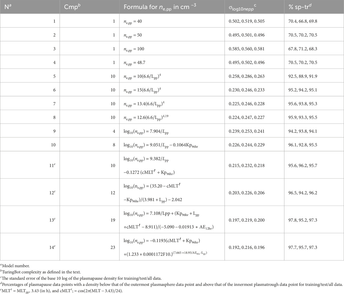
Table 2. Models for the electron density at the midpoint of the plasmapause.

For comparison, the upper dashed yellow curve in Figure 4 represents the Carpenter and Anderson (1992) plasmasphere density (summarized in item 2 of their Section 3), while the lower dashed yellow curve represents the Carpenter and Anderson plasmatrough density given by the average of the two formulas in Carpenter and Anderson’s Eq. (6) (or item 4 of their Section 3). The middle yellow dashed curve is given as follows:

$n_{\text{e,pp}}=13.4{\left(6.6/L\right)}^4{\mathrm{c}\mathrm{m}}^{-3},(6)$

which corresponds to model 7 in Table 2. This model is of the same form as Equations (1) and (2) but provides a better fit to our data as described below.

The middle and bottom thick solid gold curves in Figure 4 are fairly close to the middle and bottom dashed yellow curves, showing that the densities of our innermost plasmatrough data points are fairly close to those expected from Carpenter and Anderson’s models and that Eq. (6) is a reasonably good approximation to the L dependence of the more complicated models to be described below, especially at L ≤ 6. The upper thick solid curve in Figure 4, found from the outermost plasmasphere data points, crosses the upper yellow dashed curve from Carpenter and Anderson’s plasmasphere density model at L = 2.7 and L = 9.5 and is lower in the middle range of L values.

3.2 Modeling results

The results of our modeling are described in Table 2. Listed there are the model number, N, the TuringBot complexity, Cmp, the formulas for n_e,pp (models 1–8) or log₁₀ (n_e,pp) (models 9–14), the RMS error between the observed and model values of log₁₀ (n_e,pp), and the percentage of data points for which the model value of n_e,pp was between the density of the outermost plasmasphere data point and the innermost plasmatrough data point. In other words, the last column of Table 2 shows the percentage of model values that are within the observed range of plasmapause densities. If a model were to yield 100% in the last column of Table 2, this would mean that the model value of density would always be lower than the plasmasphere value and higher than the plasmatrough value, signifying that the model could always be depended on to separate plasmasphere and plasmatrough populations (at least for positions close to the plasmapause).

The last two columns in Table 2 have three numbers each. The first number is for the data that were used to train the models, the second number is for test data that were not used as input to the models, and the third number is for all the data. The plasmapause events were first sorted by time and then divided into 50 groups. Within each group, the middle one-sixth of the data were separated for test data in a manner similar to that of Denton et al. (2022). The purpose of this procedure was to have test data that were uncorrelated with the training data (Denton et al., 2022). The median time span of the test data intervals was 4.6 days.

The third number of three numbers in the last two columns of Table 2, respectively, showing the RMS error and percentage of events within the plasmapause for all data, including both training and test data, have values that are always intermediate between the first and second numbers. The second number for RMS error is always larger for the test data than for the training data, which is not surprising considering that the models were chosen to minimize the RMS error of the training data. However, the percentage of model values within the observed plasmapauses is sometimes greater for the training data and sometimes greater for the test data. One might reasonably take the largest RMS error and the smallest percentage of events within the plasmapause as an upper-limit measure of error.

Models 1–8 in Table 2 were motivated by the formulas that people have previously used to model the boundary between plasmasphere and plasmatrough data, either constant values in models 1–4 or power law forms in models 5–8. Model 4 is for the optimal constant value for our data set, 48.7 cm⁻³, very close to 50 cm⁻³ (model 2). For model 4, the RMS error of log₁₀ (n_e,pp) for the test data is 0.502, corresponding to a factor of 10^0.498 = 3.2, and 70.2% of the model values occur within the range of density values within the observed plasmapauses.

The use of a power law (models 5–8 in Table 2) results in significantly smaller values for the RMS error and significantly larger percentages of model values within the density range of our plasmapause events. Using the form C (6.6/Lpp)⁴ (models 5–7), the value of C = 15 cm⁻³ used by Denton et al. (2004) has a lower error and a larger percentage of model values within the observed range of plasmapause densities than does the value of C = 10 cm⁻³ used by Sheeley et al. (2001). However, the optimal value for C for our data is 13.4 (model 7), which is between 10 and 15. Based on the numbers in Table 2, there is not much benefit to letting the power law coefficient vary to its optimal value of 4.19 in model 8.

Models 9–14 show solutions from TuringBot. TuringBot finds formulas of varying complexity. We only include more complicated formulas if the TuringBot cross-validation error, our training data set error in Table 2, and our test data set error in Table 2 are less than those for formulas with lower complexity. We do not show the TuringBot cross-validation errors, but they were less than our test data errors in every case.

TuringBot did not find solutions in the form of the power laws because TuringBot’s solution with a complexity of 10 had smaller errors and larger percentages than the power law forms, which also had a complexity of 10 (this could be different if the weights for different operations were altered, but currently TuringBot does not allow that option). TuringBot’s model 10, with a complexity of 8, had comparable errors and percentages to the power law models.

The TuringBot models clearly show that the strongest dependence of n_e,pp is on L (model 9). The more complex models in Table 2 have a dependence on cMLT’ = cos (2π(MLT_pp −3.43)/24), as noted at the bottom of Table 2. The more complex models also have dependencies on F10.7 and averages of Kp and AE. The model with the lowest error in Table 2, that is, model 14, has an RMS error in log₁₀ (n_e,pp) of 0.216 for the test data, corresponding to a factor of 1.64. Model 14 yields model values of n_e,pp that are within the observed plasmapause ranges of density values for 96% of the test data.

All of the models in Table 2 also have model values within the observed range of plasmapause densities for most events. For instance, the power law form in model 7 yields model values that are within the observed range of plasmapause densities for 94% of the test data events. So from the perspective of that number, 96% for model 14, based on the test data, is only a small improvement. On the other hand, considering the number of events for which the model value is not within the observed range of plasmapause densities, the improvement in the model value from model 7 to model 14 is more significant, that is, from 6% to 4%. In other words, although the percent change in correct predictions was insignificant, the percentage of incorrect predictions was affected more significantly.

4 Discussion

The electron density at the logarithmic midpoint of the density within the plasmapause, n_e,pp, falls steeply with respect to the L value at the middle of the plasmapause, L_pp. This is obvious from the fact that density within both the plasmasphere and plasmatrough decreases steeply with respect to L (Carpenter and Anderson, 1992) and that n_e,pp must be between those densities.

Therefore, a constant value of density is a poor choice for a formula to divide plasmasphere and plasmatrough populations. Nevertheless, if one wants to use a constant value, a value of approximately 50 cm⁻³ does as well as possible, resulting in model values that are within the ranges of observed plasmapause densities for about 70% of our test data.

A power law form of $13.4{(6.6/L_{\text{pp}})}^4$ cm⁻³ does much better, finding model values that are within the ranges of observed plasmapause densities for about 94% of our test data.

The most complicated model that we found includes dependencies on MLT, F10.7, and averages over earlier times of Kp and AE. This model (model 14 in Table 2) predicts model values of n_e,pp that are within the range of observed plasmapause densities for 96% of our test data and 97% of all of our data. Returning to Figure 1A, the black circle at L = 4.6 is the prediction for the plasma density at the midpoint of the plasmapause for this event using model 14 with a typical value of AE_6h of 222 nT (since AE was not available for this event). Model 14 did a good job of predicting the density at the midpoint of the plasmapause for that event.

If one were to prefer a simpler model than model 14, the power law dependence of model 7 provides good results. Model 11 includes local time and geomagnetic activity dependence yet is still relatively simple, and like model 14, it predicts model values of n_e,pp that are within the range of observed plasmapause densities for 96% of our test data.

We wanted to test our formulas using the plasma categories in the database, for instance, to find the percentage of “plasmasphere” data points that had a density above that of model 14. Unfortunately, we found that there were a number of data points that were incorrectly categorized (we found this problem in the CRRES data, which have the highest temporal density of data points. The problem seems to involve plasmasphere and plasmatrough data points. However, we verified that this problem did not affect our plasmapause events).

Because of this problem, we were not able to compare the densities of all categories of plasma to the predictions of our formulas. However, we note that for “enhanced plasmatrough” data points with density at least a factor of 2 above surrounding plasmatrough densities (as described in the supplementary information), which we normally associate with a plasmaspheric plume, 86% of the density values were above that of model 14, showing that plume density is “plasmasphere-like” in terms of density value.

Based on the models in Table 2, n_e,pp decreases with respect to increasing L_pp and geomagnetic activity as indicated by Kp and AE, has a local maximum with respect to MLT at MLT = 15.43 h, and increases with respect to increasing F10.7. The decrease in n_e,pp with respect to increasing geomagnetic activity is reasonable, considering that greater geomagnetic activity correlates with greater magnetospheric convection (Thomsen, 2004), which sweeps density away from the earth.

The peak of n_e,pp at afternoon local time is reasonable because flux tubes refill as they convect from morning to afternoon local time (Singh and Horwitz, 1992); convection may stagnate or form a plasmaspheric plume in the late afternoon (Grebowsky, 1970; Goldstein and Sandel, 2005), and the electron density is generally higher in the afternoon (Denton et al., 2006).

We do not currently have a good explanation for why n_e,pp increases with respect to F10.7. High F10.7 correlates with a larger mass density, which does not always correlate with a larger electron density (Denton et al., 2011).

The models in Table 2, while by no means perfect, should be useful for roughly separating plasmasphere and plasmatrough populations. Not only might it be difficult to search for a steep gradient in electron density, as was performed for this study, but also magnetospheric measurements do not always encompass the plasmapause, and as mentioned before, even when the density is measured over a broad range of L, a plasmapause is not always observed. These formulas will still be useful in that case because when a plasmapause is absent, it usually indicates that the plasma is “plasmasphere-like.” This may occur either because there is an extended plasmasphere due to a long period of refilling or because there is a plasmaspheric plume that extends out from the plasmasphere in a local region. Plasmasphere-like plasma typically has a high density and is mostly composed of H+, with only low concentrations of He+ and heavy ions such as O+ for the L values that we are considering (Craven et al., 1997; Krall et al., 2008; Del Corpo et al., 2022).

Data availability statement

The geomagnetic activity indices used to create that input file are available at the NASA Goddard “OMNIWeb Plus” website, https://omniweb.gsfc.nasa.gov. The CRRES electron density data are posted at http://vmo.igpp.ucla.edu/data1/CRRES/PWE/PT8S/. Eureqa can be run online at a website provided by the DataRobot company (https://www.datarobot.com/); after a free trial period, the program is available only for monthly subscription. The TuringBot software can be found at https://turingbotsoftware.com/, and one year or lifetime licenses can be purchased. A Zenodo repository containing supplementary information including more information about our method of data classification, our (Matlab) programs, all of our electron density data, and the plasmapause event data can be found at https://zenodo.org/doi/10.5281/zenodo.10095201. The data in the Zenodo repository are described in the Supplementary Material “README.txt” document that is in the repository.

Author contributions

RD: conceptualization, data curation, formal analysis, funding acquisition, investigation, methodology, project administration, resources, software, supervision, validation, visualization, writing–original draft, and writing–review and editing. PT: conceptualization, investigation, methodology, software, visualization, and writing–review and editing. DH: writing–review and editing. JG: conceptualization and writing–review and editing. JL: software and writing–review and editing. KT: writing–review and editing.

Funding

The author(s) declare that financial support was received for the research, authorship, and/or publication of this article. RD was supported by NASA grants 80NSSC20K1446, 80NSSC21K0453, and 80NSSC19K0270.

Acknowledgments

RD is immensely grateful to the late Roger Anderson, who supplied the electron density measurements from ISEE and CRRES. Yongli Wang and Frederick Ho contributed to the research in this paper, but we were unable to contact them to invite them to be co-authors. We thank Jean-Francois Ripoli for useful conversations.

Conflict of interest

Author PT was employed by company Miraex.

The remaining authors declare that the research was conducted in the absence of any commercial or financial relationships that could be construed as a potential conflict of interest.

Publisher’s note

All claims expressed in this article are solely those of the authors and do not necessarily represent those of their affiliated organizations, or those of the publisher, the editors, and the reviewers. Any product that may be evaluated in this article, or claim that may be made by its manufacturer, is not guaranteed or endorsed by the publisher.

References

Anderson, R. R., Gurnett, D. A., and Odem, D. L. (1992). CRRES plasma-wave experiment. J. Spacecr. Rockets 29, 570–573. doi:10.2514/3.25501

CrossRef Full Text | Google Scholar

Carpenter, D. L., and Anderson, R. R. (1992). An ISEE&amp;sol;whistler model of equatorial electron density in the magnetosphere. J. Geophys. Res. 97, 1097–1108. doi:10.1029/91ja01548

CrossRef Full Text | Google Scholar

Carpenter, D. L., Anderson, R. R., Calvert, W., and Moldwin, M. B. (2000). CRRES observations of density cavities inside the plasmasphere. J. Geophys. Res. 105, 23323–23338. doi:10.1029/2000ja000013

CrossRef Full Text | Google Scholar

Craven, P. D., Gallagher, D. L., and Comfort, R. H. (1997). Relative concentration of He+ in the inner magnetosphere as observed by the DE 1 retarding ion mass spectrometer. J. Geophys. Res. 102, 2279–2289. doi:10.1029/96JA02176

CrossRef Full Text | Google Scholar

Del Corpo, A., Vellante, M., Zhelavskaya, I. S., Shprits, Y. Y., Heilig, B., Reda, J., et al. (2022). Study of the average ion mass of the dayside magnetospheric plasma. J. Geophys. Res. SPACE Phys. 127. doi:10.1029/2022JA030605

CrossRef Full Text | Google Scholar

Denton, R. E., Goldsten, J., Lee, D. H., King, R. A., Dent, Z. C., Gallagher, D. L., et al. (2006). Realistic magnetospheric density model for 29 August 2000. J. Atmos. Sol.-Terr. Phys. 68, 615–628. doi:10.1016/j.jastp.2005.11.009

CrossRef Full Text | Google Scholar

Denton, R. E., Menietti, J. D., Goldstein, J., Young, S. L., and Anderson, R. R. (2004). Electron density in the magnetosphere. J. Geophys. Res. 109. doi:10.1029/2003JA010245

CrossRef Full Text | Google Scholar

Denton, R. E., Thomsen, M. F., Takahashi, K., Anderson, R. R., and Singer, H. J. (2011). Solar cycle dependence of bulk ion composition at geosynchronous orbit. J. Geophys. Res. 116. doi:10.1029/2010ja016027

CrossRef Full Text | Google Scholar

Denton, R. E., Wang, Y., Webb, P. A., Tengdin, P. M., Goldstein, J., Redfern, J. A., et al. (2012). Magnetospheric electron density long-term (>1 day) refilling rates inferred from passive radio emissions measured by IMAGE RPI during geomagnetically quiet times. J. Geophys. Res. 117. doi:10.1029/2011ja017274

CrossRef Full Text | Google Scholar

Denton, R. E. E., Takahashi, K., Min, K., Hartley, D. P. P., Nishimura, Y., and Digman, M. C. C. (2022). Models for magnetospheric mass density and average ion mass including radial dependence. Front. Astronomy Space Sci. 9. doi:10.3389/fspas.2022.1049684

CrossRef Full Text | Google Scholar

Goldstein, J., and Sandel, B. R. (2005). “The global pattern of evolution of plasmaspheric drainage plumes,” in Inner magnetosphere interactions: new perspectives from imaging. Editors J. L. Burch, M. Schulz, and H. Spence, 1. Washington DC: American Geophysical Union).

CrossRef Full Text | Google Scholar

Grebowsky, J. (1970). Model study of plasmapause motion. J. Geophys. Res. 75, 4329–4333. doi:10.1029/JA075i022p04329

CrossRef Full Text | Google Scholar

Gurnett, D. A., Anderson, R. R., Scarf, F. L., Fredricks, R. W., and Smith, E. J. (1979). Initial results from the ISEE-1 and -2 plasma wave investigation. Space Sci. Rev. 23, 103–122. doi:10.1007/bf00174114

CrossRef Full Text | Google Scholar

Gurnett, D. A., Persoon, A. M., Randall, R. F., Odem, D. L., Remington, S. L., Averkamp, T. F., et al. (1995). The polar plasma wave instrum ent. Space Sci. Rev. 71, 597–622. doi:10.1007/bf00751343

CrossRef Full Text | Google Scholar

Krall, J., Huba, J. D., and Fedder, J. A. (2008). Simulation of field-aligned H+ and He+ dynamics during late-stage plasmasphere refilling. Ann. Geophys. 26, 1507–1516. doi:10.5194/angeo-26-1507-2008

CrossRef Full Text | Google Scholar

LeDocq, M. J., Gurnett, D. A., and Anderson, R. R. (1994). Electron number density-fluctuations near the plasmapause observed by the CRRES spacecraft. J. Geophys. Res. 99, 23661–23671. doi:10.1029/94ja02294

CrossRef Full Text | Google Scholar

Newell, P. T., Sotirelis, T., Liou, K., Meng, C. I., and Rich, F. J. (2007). A nearly universal solar wind-magnetosphere coupling function inferred from 10 magnetospheric state variables. J. Geophys. Res. 112. doi:10.1029/2006ja012015

CrossRef Full Text | Google Scholar

Qin, Z., Denton, R. E., Tsyganenko, N. A., and Wolf, S. (2007). Solar wind parameters for magnetospheric magnetic field modeling. Space weather. 5. doi:10.1029/2006SW000296

CrossRef Full Text | Google Scholar

Reinisch, B., Haines, D., Bibl, K., Cheney, G., Galkin, I., Huang, X., et al. (2000). The radio plasma imager investigation on the IMAGE spacecraft. SPACE Sci. Rev. 91, 319–359. doi:10.1023/A:1005252602159

CrossRef Full Text | Google Scholar

Schmidt, M., and Lipson, H. (2009). Distilling free-form natural laws from experimental data. Science 324, 81–85. doi:10.1126/science.1165893

PubMed Abstract | CrossRef Full Text | Google Scholar

Sheeley, B. W., Moldwin, M. B., Rassoul, H. K., and Anderson, R. R. (2001). An empirical plasmasphere and trough density model: CRRES observations. J. Geophys. Res. 106, 25631–25641. doi:10.1029/2000ja000286

CrossRef Full Text | Google Scholar

Singh, N., and Horwitz, J. L. (1992). Plasmasphere refilling - recent observations and modeling. J. Geophys. Res. 97, 1049–1079. doi:10.1029/91ja02602

CrossRef Full Text | Google Scholar

Thomsen, M. (2004). Why Kp is such a good measure of magnetospheric convection. Space Weather-The Int. J. Res. Appl. 2. doi:10.1029/2004SW000089

CrossRef Full Text | Google Scholar

Tsyganenko, N. A., and Sitnov, M. I. (2005). Modeling the dynamics of the inner magnetosphere during strong geomagnetic storms. J. Geophys. Res. 110. doi:10.1029/2004ja010798

CrossRef Full Text | Google Scholar