Quantifying adiabatic motion in the outer radiation belt and ring current with invariant matching

Adiabatic motion is a fundamental reversible process for geomagnetically trapped particle populations, including particles comprising the ring current and radiation belts. During adiabatic motion, a particle’s trajectory in configuration space responds to sufficiently slow changes in the magnetospheric magnetic field. Previous research has highlighted expected patterns in adiabatic motion, such as radial motion or the D_st effect. In this work, we introduce a method we call Invariant Matching for quantifying adiabatic motion between a pair of magnetospheres. This method can be applied to both simulation and semi-empirical magnetic field models, is computationally efficient, and in particular does not require tracing the particle trajectories. In this work, we use the Tsyganenko et al., Journal of Geophysical Research: Space Physics, 2005, 110 (TS05) magnetic field model, and present adiabatic motion between a storm commencement, the time of the storm’s D_st minimum, and a nominal recovery time. We also analyze adiabatic motion which occurs in response to enhancements of individual major current systems (including the ring current, Chapman-Ferraro current, Birkeland current, and tail current). Our methodology yields vector fields quantifying the displacement of mirror points throughout the magnetosphere, prepared in a way appropriate for application to both outer radiation belt and ring current populations.

1 Introduction

Earth’s inner magnetosphere consists of geomagnetically trapped particles, most notably the ring current and the radiation belts. At an instance in time and with a static snapshot of the global magnetic field, the particle trajectories can be described by drift shell surfaces which depend on the particles’ location, momentum, and the global geomagnetic field configuration.

The distribution of trapped particles in the inner magnetosphere depends on a balance of transport, local energization, and loss mechanisms, and can vary by orders of magnitude over time (Daglis et al., 1999; Kozyra and Liemohn, 2003; Jaynes et al., 2015; Jaynes and Usanova, 2019). Trapped particles are understood from fundamental physics and observation to undergo three periodic motions throughout their trapped trajectory: 1) gyromotion about a magnetic field line, 2) bounce motion along a field line, and 3) drift motion about the Earth. These periodic motions necessarily emerge from the trajectory described by $m\frac{d\mathbf{v}}{dt}=q(\mathbf{E}+\mathbf{v}\times \mathbf{B})$ when the particle is trapped in a dipole-like magnetic field (Chen et al., 1984). For a review of these periodic motions of geomagnetically trapped particles, see Roederer and Zhang (2016).

The trapped particle’s guiding center is confined to the surface known as its drift shell, which is subject to change as the Earth’s magnetospheric field reconfigures in response to the solar wind. When changes to these fields occur slowly, we say that the particles adjust adiabatically. That is, no work is done on the particles and the alteration to each trajectory is a reversible process within the overall magnetospheric system. Specifically, the word slowly is used to mean on time scales comparatively longer than each periodic motion (the longest of which being the drift motion period).

When this condition of slow change is met, we can also write constants of motion for the trapped particle. These quantities do not change as the trajectory in configuration space is altered. These constants of motion are known as adiabatic invariants, and are associated with the three periodic motions. The specific adiabatic invariant quantity for each periodic motion may be written in different fashions, often rewritten to create convenient properties for the analysis at hand. In this work, we use the adiabatic invariants M (corresponding to the gyromotion), K (corresponding to bounce motion), and L^* (corresponding to drift motion).

The configuration space state coordinate of a trapped particle (r, p) can be written as (M, K, L^*, φ₁, φ₂, φ₃), a vector with the same number of dimensions, where φ₁, φ₂, and φ₃ are the phases of each periodic motion (Schulz, 1996). In considering the particle’s drift shell and not its particular position within a drift shell, it is customary to drop the phase variables and simply describe the particle and its entire drift shell with the coordinate (M, K, L^*). This new phase-agnostic coordinate is powerful 1) as a fundamental state variable that is importantly invariant during slow changes to the magnetospheric magnetic field, and 2) because of its reduced number of dimensions (three versus six).

Energetic electron fluxes in the outer radiation belt are known to negatively affect satellites (Baker et al., 1994; 1998; Baker, 1998; Shea and Smart, 1998). Energetic particles pose a particular threat in which altering the state of onboard processors and circuits, potentially leading to hardware damage or the execution of unintended routines. Consequences like these can sometimes be drastic enough that they compromise the entire mission (Baker, 2002). The rate of these impacts increases with increased fluxes, and therefore it is important to pursue a detailed understanding of the dynamics behind energetic flux enhancements.

Adiabatic motion is fundamental motion in the radiation belts, with numerous applications. We will outline several of them here to motivate the study. Geostationary satellites, which orbit in circular orbits with an apogee of 6.6 R_E, are critical assets embedded in the outer radiation belt region. In the later sections of this work, we will show that within a single storm particles may move adiabatically inwards or outwards at scales up to 2 R_E. To better protect geostationary assets, we may ask: how much of the energetic particle population overlaps with geostationary orbit? We can reason that energetic particle populations interior to the geosynchronous radius of 6.6 R_E which do not initially reach these satellites may adiabatically move radially outwards until they intersect with geostationary orbit and pose a threat. Similarly, energetic particle populations currently posing a threat to geosynchronous and other satellites may move inward and create a period of safety. To best understand the time-varying energetic particle threats posted to geosynchronous satellites, we must understand these patterns of adiabatic motion.

A similar argument can be with the ring current population, and a corresponding space weather effect. In geostationary orbit, ring current particles are known to accumulate on the surface of the spacecraft, sometimes leading to spatial variation in surface charge. These spatial variations in surface charge (also known as “differential charging”) can trigger pulsed discharges harmful to on-board electronics (Lai, 2003). We can similarly ask: how does the adiabatic movement of ring current populations affect the time-dependent rate of spacecraft charging for satellites in geostationary orbit?

Adiabatic motion also has implications for research missions not in geosynchronous orbit, such as the Van Allen Probes (Mauk et al., 2014). The Van Allen Probes satellites orbited with an apogee of about 5.8 R_E, which serves as a radial upper bound for the mission’s outer radiation belt coverage. However, because particles are known to adiabatically move inwards and outwards radially, they will inevitably transition in and out of the satellite’s coverage. The extent to which this occurs is relevant to studies using such data, and the interpretation of outer radiation belt data.

Finally, we consider an application between adiabatic motion and induced field changes from the ring current. The ring current is the primary source of magnetic field depletion at the Earth’s surface during geomagnetic storms, whose strength is often stated in terms of the D_st index. The induced change to the magnetospheric magnetic fields caused by the ring current can be calculated with the Biot-Savart law (Yu and Ridley, 2008), $\mathrm{\Delta }\mathbf{B}(\mathbf{r})=\frac{{\mu }_0}{4\pi }{\iiint }_{\text{RingCurrent}}\frac{\mathbf{J}\times {\mathbf{r}}^{\prime }}{|{\mathbf{r}}^{\prime }{|}^3}dV$, where-in the change from magnetic field ΔB due to the ring current is calculated through an integral over the ring current region, with current density J, positions r and r′, and infinitesimal volume dV. In this equation we bring attention to the 1/|r′|³ term, which shows that the ΔB at a location in the magnetosphere is connected to its distance to each infinitesimal volume of the ring current having a notable current density. This change in the magnetic field strength due to changes in the ring current will alter the drift shells of trapped energetic particles.

In this work, we quantify the adiabatic motion using a method centered around the theory of adiabatic invariants. Our method, which we call Invariant Matching, pairs mirror points of equal K and L* over space from distinct magnetospheres. This can be viewed through the lens of a particle’s drift shell adapting in shape to conserve K and L* under newly encountered fields. We note that K and L* alone dictate the drift shell structure because, for our considered populations, the gyro-radius is extremely small compared to the spatial scales of the bounce and drift motions.

Our method is a computationally efficient alternative to particle tracing when adiabatic motion that is free from non-adiabatic effects is considered. While it is well understood that non-adiabatic effects occur in nature, the results which originate from our method can be interpreted as theoretical features pertaining to fundamental transitional behaviour between pairs of magnetospheres. We call this pure adiabatic motion between two sets of global magnetic fields idealized adiabatic motion to emphasize the calculation’s independence from any non-adiabatic effects.

In this work, we model and discuss idealized adiabatic motion during a geomagnetic storm using the semi-empirical magnetic field model driven by L₁ solar wind measurements and the D_st index. We quantify the adiabatic displacement of mirror points between a storm time commencement, time of D_st minimum, and nominal recovery time to understand how particles move adiabatically within a storm.

Because changes to the global magnetic field are completely driven by currents throughout the magnetosphere, we also study the adiabatic response to individual current system enhancements. The current systems we study are the ring current, tail currents, Birkeland currents, and Chapman-Ferraro currents. Specifically, we vary each current system individually, and observe the adiabatic response. Because these currents ultimately drive each major distortion of the global magnetosphere magnetic field, it is useful to gain a sense of their respective contributions to adiabatic motion.

2 Models

To model the global magnetospheric magnetic field, we use the Tsyganenko/Sitnov 2005 (TS05) model. This semi-empirical model of the global magnetospheric magnetic field combines both physical modeling and a history of satellite observation in a comprehensive modeling approach refined over multiple decades (Tsyganenko, 1991; Tsyganenko, 1996; Tsyganenko, 2002a; Tsyganenko, 2002b; Tsyganenko and Mukai, 2003; Tsyganenko and Sitnov 2005). Interior to the magnetopause, this model calculates the overall magnetic field B_Final as the sum of seven contributing vectors,

${\mathbf{B}}_{\text{Final}}={\mathbf{B}}_{\text{CF}}+{\mathbf{B}}_{\mathrm{T}\mathrm{A}\mathrm{I}\mathrm{L}\mathrm{1}}+{\mathbf{B}}_{\mathrm{T}\mathrm{A}\mathrm{I}\mathrm{L}\mathrm{2}}+{\mathbf{B}}_{\text{SRC}}+{\mathbf{B}}_{\text{PRC}}+{\mathbf{B}}_{\mathrm{B}\mathrm{I}\mathrm{R}\mathrm{K}\mathrm{1}}+{\mathbf{B}}_{\mathrm{B}\mathrm{I}\mathrm{R}\mathrm{K}\mathrm{2}}+{\mathbf{B}}_{\text{IMF}},(1)$

where B_CF represents the contribution from the Chapman-Ferraro current system, B_TAIL1 and B_TAIL2 from two regions of tail currents, B_SRC from the “symmetric” ring current, B_PRC from the “partial” ring current, B_BIRK1 and B_BIRK2 from two regions of the Birkeland currents, and B_IMF from the penetrated component of the interplanetary magnetic field (IMF). We note that the penetrated component, unlike the others, does not nominally correspond to a magnetospheric current system for the purposes of this paper.

Tsyganenko and Sitnov (2005) describe their rationale for splitting some current systems into two terms. For the tail currents, two distinct tail current regions are used to separately model inner and outer cross-tail current. Two Birkeland currents allow for shifting the current peaks longitudinally, where Region 1 corresponds to current peaks at dawn and dusk and Region 2 corresponds to current peaks at noon and midnight. The symmetric ring current differs from the partial ring current in that the symmetric ring current is axially symmetric, while the partial ring current includes the effects of field-aligned currents associated with the local time asymmetry of azimuthal near-equatorial currents (Tsyganenko, 2002b).

In Figure 1 we display time-varying metrics for current system intensity for three current groups during the geomagnetic storm beginning on 2 October 2013: the ring current (B_PRC and B_SRC), tail current (B_TAIL1 and B_TAIL2), and Birkeland currents (B_BIRK1 and B_BIRK2). This demonstrates how the intensity of each current system varies overall on a scale of about 4X between the quiet time intensity and the intensity during the storm’s D_st minimum. This plot is prepared with the total current integrated over a surface using the equation,

$\mathrm{T}\mathrm{o}\mathrm{t}\mathrm{a}\mathrm{l}\mathrm{C}\mathrm{u}\mathrm{r}\mathrm{r}\mathrm{e}\mathrm{n}\mathrm{t}=\iint \frac{1}{{\mu }_0}|\nabla \times \sum {\mathbf{B}}_{\mathbf{i}}|dA,(2)$

where B_i are the magnetic field vectors from the terms considered. The integration surface used is the midnight X-Z plane bounded by X > − 20 R_E (Solar Magnetic coordinates) for the ring current and tail current. The integration surface for the Birkeland current is the X-Y plane at Z = 1.1 R_E, to place the surface where the Birkeland currents take their field-align direction.

Figure 1

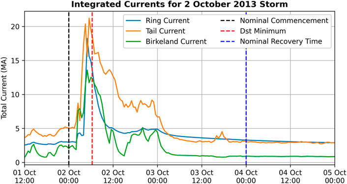
Figure 1. Integrated currents over the course of a geomagnetic storm, showing variation on a scale of about 4X between the quiet-time intensity and the intensity at the time of D_st minimum.

The model itself computes each of the contributing vectors as a function of upstream solar wind conditions and geomagnetic state. Specifically, the input variables are the IMF B_y and B_z, the D_st index, the interplanetary dynamic pressure P_dyn, and six time-dependent parameters W₁ to W₆ that allow the model to account for the growth and decay of persistent currents. In this work, the QinDenton dataset is used to supply the TS05 inputs, including the W parameters (Qin et al. (2007); data sourced from http://mag.gmu.edu/ftp/QinDenton/5min/merged/latest/).

In this work, we investigate the adiabatic responses of ring current and radiation belt particles to individual current systems. An illustration of the combined current sources can be found in Figure 2, which shows the current density calculated from the equation

$J_{\mathit{ext}}=\frac{1}{{\mu }_0}|\nabla \times {\mathbf{B}}_{\mathbf{ext}}|,(3)$

where B_ext is the external magnetic field vector obtained from TS05, J_ext is the current density associated with the perturbed (non-dipole) fields, and μ₀ is the vacuum magnetic permeability. This example is driven by the inputs P_dyn = 1.64 nPa, D_st = −7.0 nT, B_y = −2.7 nT, B_z = −1.2 nT, W₁ = 0.338, W₂ = 0.469, W₃ = 0.063, W₄ = 0.248, W₅ = 0.337 and W₆ = 0.58. These inputs correspond to the commencement time of the storm that will be described later in this article. In this plot, we see a complex description of the global magnetosphere, including multiple layers of ring current, a tail current, and cavities of current density immediately around the polar regions.

Figure 2

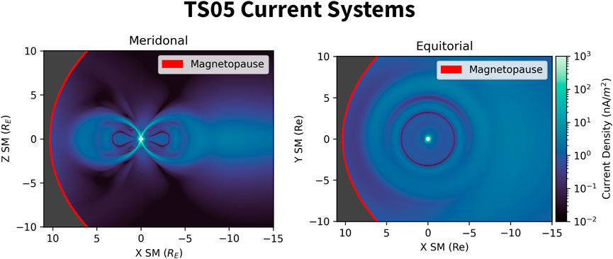
Figure 2. Model cuts displaying the current systems extracted from the Tsyganenko/Sitnov 2005 (TS05) model, using Equation 3

Our work will investigate the influence of individual current systems by artificially scaling terms of Eq. 1 to enhance each system. This is implemented using a modified version of the official Fortran TS05 code, available at https://geo.phys.spbu.ru/∼tsyganenko/empirical-models/magnetic_field/ts05/. Specifically, the function which holds the code that adds together the contributing terms is modified to accept scale factors used to multiply each contributing term.

3 Methods

We seek to describe the adiabatic motion of ring current and radiation belt particles between a pair of magnetospheres. The key state of a trapped particle is its adiabatic invariant coordinate (M, K, L^*) that describes its trapped state. For the purposes of this manuscript, we will accept that the three adiabatic invariant coordinates (M, K, L^*) can be calculated in conjunction with a magnetic field model from a starting position ×₀, a particle rest mass m₀, and mirroring field intensity B_m. Readers interested in the details of the calculation used are referred to da Silva et al. (2023).

The approach used is to associate particles mirroring at a known point along a fixed drift shell, and through computational methods, match them to the mirror point under a new drift shell they would adiabatically transition to under a modified global magnetic field, in the absence of any non-adiabatic effects such as wave-particle interactions. We calculate the idealized adiabatic motion between a starting magnetosphere and an ending magnetosphere. The approach begins by preprocessing the ending global magnetic field. A grid of positions on an X-Z slice of Solar Magnetic (SM) space are associated with adiabatic coordinates (K, L^*) corresponding to a particle which mirrors there. This produces a “mapped” dataset which maps a grid of mirror positions (X_ij, Z_ij) to adiabatic coordinates $(K_{ij},L_{ij}^{*})$.

The invariant matching grid is irregular, and formed by varying the L-shell variable L between 2.5 and 9.0 (in increments of 0.1), and the magnetic latitude ϕ of a mirror point along each field line between −61° and 61° (in increments of 2°) with extra points placed at ± 0.1° around the equator. These extra points were placed to extend the minimum K which could be interpolated. Each mirror point magnetic latitude, whether positive or negative, yields the mirroring field strength B_m, which inherently specifies the opposite mirror point location along that field line. This grid is designed to cover the region of space occupied by outer radiation belt elections and include a variety of mirroring states. Through this mapping process each of the (L, ϕ) grid points is connected to a (K, L^*) coordinate.

The mapped dataset describing the ending magnetosphere is used to match adiabatic coordinates (K, L^*) from the starting magnetosphere with the mirror point locations in the ending magnetosphere. For each mirror point in the starting magnetosphere, the mapped dataset is interpolated to find the corresponding (X, Z) position where the mirror points displace to in the ending magnetosphere. In Figure 3 we show the adiabatic coordinates of the mapped ending magnetosphere mirror points colored by their X and Z coordinates, with the adiabatic coordinates of the starting magnetosphere mirror points as black/white circles.

Figure 3

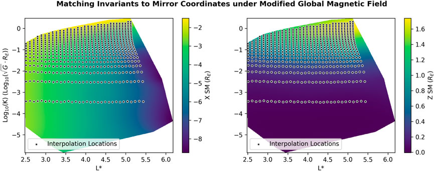
Figure 3. Adiabatic invariant coordinates (K, L*) in the ending magnetosphere are computed for particles mirroring on a grid of L and magnetic latitude ϕ at a fixed local time. The X and Z variables correspond to the SM mirror point location at the local time. This mapping (K, L*)↦(X, Z) is interpolated to find the location of the mirror point for a $(K_0,L_0^{*})$ particle originating from the starting magnetosphere.

The interpolation done is in the log-scale for the K coordinate, which naturally spans about 7 orders of magnitude. To interpolate, a radial basis function method is used from the SciPy package (Virtanen et al., 2020). Specifically, we use multiquadratic basis functions of the form $b(r)=\sqrt{{(r/ϵ)}^2+1}$ where b(r) is the radial basis function, r is the radius, and ϵ is equal to the average distance between data points. The smoothness setting is used to force the interpolation function to always go through the data points. This method was chosen because of its effectiveness working with scattered data. Care is taken to not extrapolate the mapped dataset; if at any time one of the interpolation locations is not fully within the enclosed bounds of the mapped data points then the adiabatic motion is not computed. This constraint is accomplished by checking whether the interpolation location is within the convex hull of the mapped data points.

We now discuss the scope of this methodology. This methodology may be applied where the three invariants are conserved for the particles in question. Previous studies of trapped particle motion have identified a number of cases where the invariants are not conserved, which we review here. Generally speaking, if M is not conserved, then K and L^* are also not conserved, and if K is not conserved, L^* is not. Known scenarios where one or more invariants are broken include.

• Highly curved field lines, where the gyro radius approaches the curvature radius of the field line.

• Spatially sheared field lines, where there is a sudden large change in field line direction over space, such as around the magnetotail current sheet.

• Drift Orbit Bifurcation (DOB), such as around the dayside Shabansky region.

• Rapid changes to the magnetic field topology, such as where there the global magnetic topology alters the motion of the particle on a scale faster than the drift period.

• Large gradients in the field line strength, such as around the magnetopause and magnetosheath boundary layer (MSBL).

• Resonant Wave-Particle Interactions, such as but not limited to chorus or ULF waves.

Detailed discussion of each of these scenarios is outside the scope of this paper. For issues regarding curvature of field lines, see Anderson et al. (1997). For matters of the magnetotail see Anderson et al. (1997). For wave-particle interactions see Ukhorskiy et al. (2006) and Elkington et al. (2003) when concerned with ULF waves, and An et al. (2022) for chorus waves.

4 Results

4.1 Idealized adiabatic motion between storm times

We now turn our attention to studying the idealized adiabatic motion during a geomagnetic storm, nominally beginning on 2 October 2013. This storm, previously studied in da Silva et al. (2023), was triggered by a coronal mass ejection (CME) (NASA, 2013) with mostly $B_y^{\mathit{IMF}}<0$ plasma and flow speeds in excess of 600 km/s. The magnetosphere’s response reached a minimum D_st of −90 nT during the peak of the storm.

We study the idealized adiabatic motion between three times in the storm: 1) a nominal commencement time immediately preceding the CME, 2) the time of minimum D_st, chosen to reflect the most disturbed state, and 3) a nominal recovery time about 2 days after the commencement, when the solar wind dynamic pressure had since returned to its baseline value and there no longer existed a strong southward $B_z^{\mathit{IMF}}$.

Though it is generally understood that adiabatic breaking behaviour would occur between the commencement and main phase, we apply this method to a storm to demonstrate the scale of adiabatic influence. The adiabatic motion between the storm commencement and the time of D_st minimum is displayed in the top panel of Figure 4. Each of the vectors drawn in this plot is between a mirror point in the commencement magnetosphere and its corresponding adiabatically displaced mirror point in the D_st minimum magnetosphere. The bottom two panels show the external current densities (from all external current sources) for each magnetosphere computed using Eq. 3. The commencement magnetospheric field lines are drawn in white, and the D_st minimum field lines are drawn in gray.

Figure 4

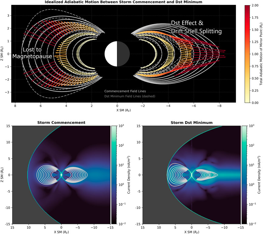
Figure 4. Idealized adiabatic motion between a nominal storm commencement time and the time of D_st minimum for the storm, displayed through the displacement of mirror points. The bottom two panels show the total external field current density, computing using Eq. 3.

We notice a number of interesting features in these plots. The magnitude of the adiabatic mirror point displacement is largest furthest away from the Earth, where the external field dominates. As expected, the D_st minimum dayside magnetosphere is significantly more compressed than during the storm commencement. On the dayside, we also see that the adiabatic displacement of the mirror points tends to be broadly in the direction perpendicular to the field line. We label a region around the magnetic equator where the adiabatic motion would have displaced mirror points past the magnetopause, in a well-understood phenomena known as magnetopause shadowing or magnetopause incursion (Jaynes and Usanova, 2019). Magnetopause shadowing affects particles in pitch angle bands around 90°. Through the dropouts of particles in these pitch angle bands, the phenomena is known to instigate doubly-peaked “butterfly” pitch angle distributions. The features observed here are consistent with test particle simulations of magnetopause shadowing (Saito et al., 2010), Fokker-Planck simulations (Yu et al., 2013), and phase space density observations (Staples et al., 2022; Turner et al., 2013; Shprits et al., 2012; Loto’Aniu et al., 2010; Sibeck et al., 1987).

Moving on the tail portion of Figure 4, we observe a combined influence of the Dst effect and drift shell splitting. we label L-shell spreading. The experiment depicts latitude-dependent outward mirror-point displacement within the same starting field line (attributable to drift shell splitting), with the strongest displacement just outside the ring current region (widely known as the Dst effect). There are two peaks in total displacement magnitude at roughly the same absolute magnetic latitude. This can be expected to lead to interesting changes in the equatorial pitch angle distributions as would be measured at increasing L values into the tail. That is, the equatorial pitch angle distribution versus L would change in shape/structure from particles being exchanged in pitch angle dependent amounts across L-shells.

The adiabatic motion between the D_st minimum for the storm and the nominal recovery time over 36 h later is displayed in Figure 5. We note signatures of a well known phenomena known as drift orbit bifurcation (DOB). This phenomenon occurs in a region of the dayside magnetic field known as the Shabansky region (Shabansky, 1971; McCollough et al., 2012). In the Shabansky region, each magnetic field line is “hammer-head” shaped as it contains two local minima in magnetic field strength. Each of these local minima is located near each cusp (Öztürk and Wolf, 2007). Test particle simulations have confirmed that when particles of sufficiently low B_m pass through these regions they become trapped within one of the two local minima, with the minimum chosen being effectively stochastic.

Figure 5

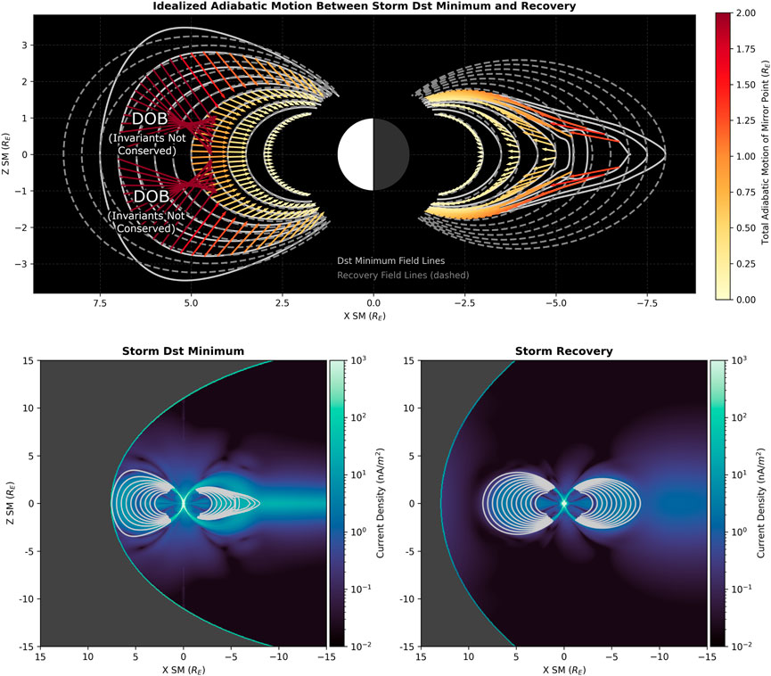
Figure 5. Idealized adiabatic motion between the time of minimum D_st for the storm and a nominal recovery time over 36 h later, displayed through the displacement of mirror points. DOB stands for drift orbit bifurcation. The bottom two panels show the total external field current density, computed using Eq. 3.

In Figure 5, we observe the results of invariant matching on the dayside for drift shell mirror points subject to DOB effects at the time of D_st minimum but not during recovery. The pitch angle dependent dynamics of entering and leaving the Shabansky region have been reported in McCollough et al. (2012). McCollough et al.’s work describes three types of particles encountering the region, labeled as Type I, II, and III. Type I particles are those of high K that undergo dayside drifts without mirroring inside the bifurcated region; in many ways they are unaffected by the unique Shabansky structure. Type II and III particles are those which mirror inside the bifurcated region, spending their time at high latitudes while in the Shabansky region. The difference between Type II and III particles is that Type II particles have small K (which is conserved after leaving the Shabansky region), and Type III particles have an even smaller near-zero K (which is not conserved after leaving the Shabansky region). While mirroring inside the Shabansky region, a standard prescription is that the full value of K is partitioned between minima, such that K = K₁ + K₂. It is common, though not entirely accurate, to approximate K₁ and K₂ with K₁ = K₂ = K/2.

Our model of idealized adiabatic motion accurately describes Type I and II particles, but less so for Type III particles. This is necessarily because K, and therefore L^*, are not conserved after leaving the region for Type III particles, which violates a key assumption of the Invariant Matching method. The arrow crossing in Figure 5 can be understood to occur at the mirroring latitudes which effectively act as classification boundaries between Type I and II particles. We note that a similar but reversed DOB effect occurred between commencement and D_st minimum for particles drifting on the dayside around L = 6 in the commencement magnetosphere, but it was cropped out of Figure 4 for visual simplicity. We note that the changes to K and L^* for Type III particles were reported in McCollough et al. (2012) be small within a drift.

Their work showed at each drift, K about doubled in value when entering/exiting the Shabansky region a single time. This is notably small compared to the seven orders of magnitude of K across a field line observed in our work (Figure 3). It was reported in that work that this per-drift change in K and L^* would repeat in the form of a diffusive process. For this reason, we do not claim exact results for near-equatorial Type III particles in the Shabansky region.

4.2 Idealized adiabatic motion in response to current system enhancements

Using this method as our tool of study, we now turn our attention to the relative role of magnetospheric current systems on adiabatic motion. We perform experiments for each of four major current systems: the ring current, the tail current, the Chapman-Ferraro current, and the Birkeland current. As outlined in Eq. 1, the ring current corresponds to the field source terms B_PRC and B_SRC, the tail current to B_TAIL1 and B_TAIL2, the Chapman-Ferraro current to B_CF, and the Birkeland current to B_BIRK1 and B_BIRK2,

In this experiment, we use a nominal magnetosphere taken during the storm commencement (labeled in Figure 1) as the starting magnetosphere. For the ending magnetosphere, we double the intensity of the major current system being studied. This is done by doubling the corresponding field source terms in Eq. 1. For example, when we compute a magnetosphere with a double the ring current intensity, we compute a new magnetosphere with the B_PRC + B_SRC terms replaced with 2(B_PRC + B_SRC), leaving the other terms the same.

The purpose of this exercise is to understand the adiabatic response of radiation belt and ring current particles to enhancements of each major current system. In Figure 1’s display of integrated currents throughout a storm, we notice that the relative intensity of each current group varies throughout the storm. For example, we notice that while both the tail current and the ring current reach their maximum intensity around the time of D_st minimum, the ring current intensity in the model drops more rapidly than the tail current. By analyzing the adiabatic responses to each major current system, we move towards a more detailed understanding of the adiabatic responses throughout a storm on hourly time scales.

In Figure 6, we observe the effect of doubling the ring current intensity in our nominal magnetosphere. This enhancement results in outward displacement of mirror points on both the nightside and dayside. We observe that the vertical change Δz in the mirror point location is small on the nightside, but latitude-dependent on the dayside. On the dayside outer most field line with vectors plotted, we see the adiabatic motion begin to point to rearrangements (on the equator) around the equator corresponding to DOB. This result indicates that a ring current enhancement of the magnitude, alone, is enough to displace particles onto the DOB field lines, without any compression of the magnetosphere. This is notable, as it reminds us that ring current enhancement can push higher L particles into this region, even with a steady magnetopause location.

Figure 6

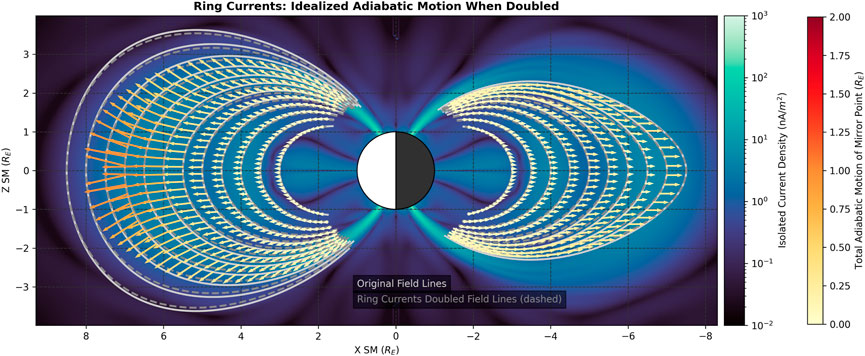
Figure 6. Idealized adiabatic motion when the ring current intensity is doubled. The background shows the external field density consisting of just the ring current source terms, computed using Eq. 3.

The adiabatic effects of doubling of the Chapman-Ferraro current, displayed in Figure 7, shows a different story. This current doubling, which has a notable effect on the shape of the dayside field lines, overall results in inward mirror point displacement, with minimal Δz vertical movement on both the dayside and the nightside.

Figure 7

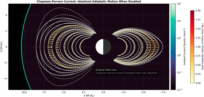
Figure 7. Idealized adiabatic motion when the Chapman-Ferarro current intensity is doubled. The background shows the external field density consisting of just the Chapman-Ferarro source, computed using Eq. 3.

The effects of the tail current, displayed in Figure 8, show largely outward motion. On the dayside, the Δz of the mirror point displacement is clearly latitude dependent, with more Δz at higher magnetic latitudes. On the nightside, this relationship between magnetic latitude and Δz is missing lower at L, and at higher L is overcome by effects of the tail stretching.

Figure 8

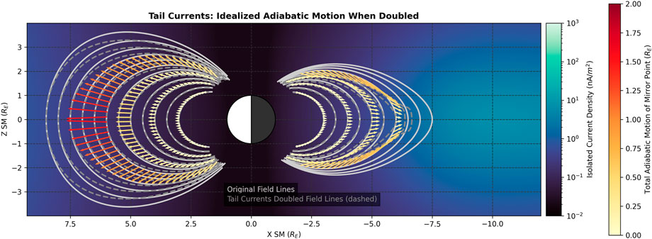
Figure 8. Idealized adiabatic motion when the tail current intensity is doubled. The background shows the external field density consisting of just the tail current source terms, computed using Eq. 3.

Similar to the other analysis, the effects of the Birkeland current is also analyzed. It was found that when doubled, the adiabatic response to the Birkeland current is extremely small and most likely negligible compared to these other current systems.

5 Conclusion

In this work we present a new method for quantifying adiabatic motion for particles in the radiation belts and ring current. Our method works by tracking the displacement of mirror points, pairing a starting mirror point with its ending location using a mapped version of the ending magnetosphere. This approach makes it easy to compute and visualize vector fields corresponding to the displacement of mirror points throughout the magnetosphere. Though not pictured here, this method could be applied to the dawn/dusk local times in addition to noon and midnight.

Results from this method yield features such as magnetopause shadowing, drift orbit bifurcation, and a combination of the Dst effect and drift shell splitting. Phenomena we label as L-shell spreading. These features are found consistent with existing observations and test particle simulations in the literature (Saito et al., 2010; Yu et al., 2013; Staples et al., 2022; Turner et al., 2013; Shprits et al., 2012; Loto’Aniu et al., 2010; Sibeck et al., 1987), serving as a simple validation of the method.

In particular, the drift orbit bifurcation patterns can be explained by displacement to conserve B_m during a transition from Shabansky field line to a normal field line. In our observations of magnetopause shadowing, we observed how invariant matching can capture the effects of drift shells displacing past the magnetopause. The observation of L-shell spreading indicates that particles which once collocate a single field line at a given MLT can become spread out across multiple field lines at that MLT from adiabatic effects alone.

The magnetospheric system’s adiabatic response to enhancements of individual current systems was also analyzed. We looked at current groups as modeled through the TS05 model, including the ring current, the Chapman-Ferraro current, the tail current, and the Birkeland current. We noted that enhancements in the ring current and tail currents generates outward motion, an enhancement to the Chapman-Ferraro current generates inward motion, and the effect of the Birkeland current is largely negligible.

This work has presented analyses of adiabatic responses to storm-time magnetospheric deformations and responses to individual current system enhancements, which are important analysis tools to begin with when applying the method. Future potential applications include complementing existing modeling using this independent method which has the bonus of being more computationally efficient. Topics include modeling of magnetopause shadowing, such as quantifying the span of pitch angles at each L which undergo loss after an adiabatic response due to a changing location of the magnetopause. Other applications include addressing the topics mentioned in the introduction: 1) geosynchronous satellite vulnerability to single event effects and spacecraft charging, 2) outer radiation belt coverage for observational satellites like the Van Allen Probes, and 3) changes to B at Earth and throughout the inner magnetosphere due to displacement of the ring current.

Data availability statement

Publicly available datasets were analyzed in this study. This data can be found here: Zenodo repository, https://doi.org/10.5281/zenodo.11089801. The Qin-Denton dataset with OMNI parameters can be found at: https://rbsp-ect.newmexicoconsortium.org/data_pub/QinDenton/.

Author contributions

DD: Conceptualization, Data curation, Formal Analysis, Funding acquisition, Investigation, Methodology, Software, Validation, Visualization, Writing–original draft, Writing–review and editing. SE: Funding acquisition, Investigation, Supervision, Writing–original draft, Writing–review and editing. MH: Writing–original draft, Writing–review and editing.

Funding

The author(s) declare that financial support was received for the research, authorship, and/or publication of this article. NASA FINESST Grant.

Conflict of interest

The authors declare that the research was conducted in the absence of any commercial or financial relationships that could be construed as a potential conflict of interest.

Publisher’s note

All claims expressed in this article are solely those of the authors and do not necessarily represent those of their affiliated organizations, or those of the publisher, the editors and the reviewers. Any product that may be evaluated in this article, or claim that may be made by its manufacturer, is not guaranteed or endorsed by the publisher.

References

An, Z., Wu, Y., and Tao, X. (2022). Electron dynamics in a chorus wave field generated from particle-in-cell simulations. Geophys. Res. Lett. 49, e2022GL097778. doi:10.1029/2022gl097778

CrossRef Full Text | Google Scholar

Anderson, B., Decker, R., Paschalidis, N., and Sarris, T. (1997). Onset of nonadiabatic particle motion in the near-earth magnetotail. J. Geophys. Res. Space Phys. 102, 17553–17569. doi:10.1029/97ja00798

CrossRef Full Text | Google Scholar

Baker, D. (1998). What is space weather? Adv. Space Res. 22, 7–16. doi:10.1016/s0273-1177(97)01095-8

CrossRef Full Text | Google Scholar

Baker, D., Allen, J., Kanekal, S., and Reeves, G. (1998). Disturbed space environment may have been related to pager satellite failure. Eos, Trans. Am. Geophys. Union 79, 477–483. doi:10.1029/98eo00359

CrossRef Full Text | Google Scholar

Baker, D., Kanekal, S., Blake, J., Klecker, B., and Rostoker, G. (1994). Satellite anomalies linked to electron increase in the magnetosphere. Eos, Trans. Am. Geophys. Union 75, 401–405. doi:10.1029/94eo01038

CrossRef Full Text | Google Scholar

Baker, D. N. (2002). How to cope with space weather. Science 297, 1486–1487. doi:10.1126/science.1074956

PubMed Abstract | CrossRef Full Text | Google Scholar

Chen, F. F. (1984) Introduction to plasma physics and controlled fusion. Springer.

Google Scholar

Daglis, I. A., Thorne, R. M., Baumjohann, W., and Orsini, S. (1999). The terrestrial ring current: origin, formation, and decay. Rev. Geophys. 37, 407–438. doi:10.1029/1999rg900009

CrossRef Full Text | Google Scholar

da Silva, D., Elkington, S. R., Li, X., Murphy, J., Wiltberger, M. J., Chan, A. A., et al. (2023). Numerical calculations of adiabatic invariants from MHD-driven magnetic fields (under revision). J. Geophys. Res. Space Phys. XXX, XXX.

Google Scholar

[Dataset] NASA(2013). Aurora in New York on oct. 2, 2013. Available at: https://www.nasa.gov/image-article/aurora-new-york-oct-2-2013/.

Google Scholar

Elkington, S. R., Hudson, M. K., and Chan, A. A. (2003). Resonant acceleration and diffusion of outer zone electrons in an asymmetric geomagnetic field. J. Geophys. Res. Space Phys. 108. doi:10.1029/2001ja009202

CrossRef Full Text | Google Scholar

Jaynes, A., and Usanova, M. (2019) The dynamic loss of Earth’s radiation belts: from loss in the magnetosphere to particle precipitation in the atmosphere. Elsevier.

Google Scholar

Jaynes, A. N., Baker, D. N., Singer, H. J., Rodriguez, J. V., Loto’Aniu, T., Ali, A., et al. (2015). Source and seed populations for relativistic electrons: their roles in radiation belt changes. J. Geophys. Res. Space Phys. 120, 7240–7254. doi:10.1002/2015ja021234

CrossRef Full Text | Google Scholar

Kozyra, J. U., and Liemohn, M. W. (2003). “Ring current energy input and decay,” in Magnetospheric imaging—the image prime mission (Springer), 105–131.

CrossRef Full Text | Google Scholar

Lai, S. T. (2003). A critical overview on spacecraft charging mitigation methods. IEEE Trans. Plasma Sci. 31, 1118–1124. doi:10.1109/tps.2003.820969

CrossRef Full Text | Google Scholar

Loto’Aniu, T., Singer, H., Waters, C., Angelopoulos, V., Mann, I., Elkington, S., et al. (2010). Relativistic electron loss due to ultralow frequency waves and enhanced outward radial diffusion. J. Geophys. Res. Space Phys. 115. doi:10.1029/2010ja015755

CrossRef Full Text | Google Scholar

Mauk, B., Fox, N. J., Kanekal, S., Kessel, R., Sibeck, D., and Ukhorskiy, a. A. (2014) Science objectives and rationale for the radiation belt storm probes mission. The van Allen probes mission, 3–27.

Google Scholar

McCollough, J., Elkington, S., and Baker, D. (2012). The role of shabansky orbits in compression-related electromagnetic ion cyclotron wave growth. J. Geophys. Res. Space Phys. 117. doi:10.1029/2011ja016948

CrossRef Full Text | Google Scholar

Öztürk, M. K., and Wolf, R. A. (2007). Bifurcation of drift shells near the dayside magnetopause. J. Geophys. Res. Space Phys. 112. doi:10.1029/2006ja012102

CrossRef Full Text | Google Scholar

Qin, Z., Denton, R., Tsyganenko, N., and Wolf, S. (2007). Solar wind parameters for magnetospheric magnetic field modeling. Space weather. 5. doi:10.1029/2006sw000296

CrossRef Full Text | Google Scholar

Roederer, J. G., and Zhang, H. (2016) Dynamics of magnetically trapped particles. Springer.

Google Scholar

Saito, S., Miyoshi, Y., and Seki, K. (2010). A split in the outer radiation belt by magnetopause shadowing: test particle simulations. J. Geophys. Res. Space Phys. 115. doi:10.1029/2009ja014738

CrossRef Full Text | Google Scholar

Schulz, M. (1996). Canonical coordinates for radiation-belt modeling. Radiat. Belts Models Stand. 97, 153–160. doi:10.1029/gm097p0153

CrossRef Full Text | Google Scholar

Shabansky, V. (1971). Some processes in the magnetosphere. Space Sci. Rev. 12, 299–418. doi:10.1007/bf00165511

CrossRef Full Text | Google Scholar

Shea, M., and Smart, D. (1998). Space weather: the effects on operations in space. Adv. Space Res. 22, 29–38. doi:10.1016/s0273-1177(97)01097-1

CrossRef Full Text | Google Scholar

Shprits, Y., Daae, M., and Ni, B. (2012). Statistical analysis of phase space density buildups and dropouts. J. Geophys. Res. Space Phys. 117. doi:10.1029/2011ja016939

CrossRef Full Text | Google Scholar

Sibeck, D., McEntire, R., Lui, A., Lopez, R., and Krimigis, S. (1987). Magnetic field drift shell splitting: cause of unusual dayside particle pitch angle distributions during storms and substorms. J. Geophys. Res. Space Phys. 92, 13485–13497. doi:10.1029/ja092ia12p13485

CrossRef Full Text | Google Scholar

Staples, F. A., Kellerman, A., Murphy, K. R., Rae, I. J., Sandhu, J. K., and Forsyth, C. (2022). Resolving magnetopause shadowing using multimission measurements of phase space density. J. Geophys. Res. Space Phys. 127, e2021JA029298. doi:10.1029/2021ja029298

PubMed Abstract | CrossRef Full Text | Google Scholar

Tsyganenko, N. (1991). Methods for quantitative modeling of the magnetic field from birkeland currents. Planet. space Sci. 39, 641–654. doi:10.1016/0032-0633(91)90058-i

CrossRef Full Text | Google Scholar

Tsyganenko, N. (2002a). A model of the near magnetosphere with a dawn-dusk asymmetry 1. mathematical structure. J. Geophys. Res. Space Phys. 107, SMP–12. doi:10.1029/2001ja000219

CrossRef Full Text | Google Scholar

Tsyganenko, N. (2002b). A model of the near magnetosphere with a dawn-dusk asymmetry 2. parameterization and fitting to observations. J. Geophys. Res. Space Phys. 107, SMP–10. doi:10.1029/2001ja000220

CrossRef Full Text | Google Scholar

Tsyganenko, N., and Mukai, T. (2003). Tail plasma sheet models derived from geotail particle data. J. Geophys. Res. Space Phys. 108. doi:10.1029/2002ja009707

CrossRef Full Text | Google Scholar

Tsyganenko, N., and Sitnov, M. (2005). Modeling the dynamics of the inner magnetosphere during strong geomagnetic storms. J. Geophys. Res. Space Phys. 110. doi:10.1029/2004ja010798

CrossRef Full Text | Google Scholar

Tsyganenko, N. A. (1996). Effects of the solar wind conditions in the global magnetospheric configurations as deduced from data-based field models. Int. Conf. substorms 389, 181. doi:10.1029/96JA02735

CrossRef Full Text | Google Scholar

Turner, D., Angelopoulos, V., Li, W., Hartinger, M., Usanova, M., Mann, I., et al. (2013). On the storm-time evolution of relativistic electron phase space density in earth’s outer radiation belt. J. Geophys. Res. Space Phys. 118, 2196–2212. doi:10.1002/jgra.50151

CrossRef Full Text | Google Scholar

Ukhorskiy, A., Anderson, B., Takahashi, K., and Tsyganenko, N. (2006). Impact of ulf oscillations in solar wind dynamic pressure on the outer radiation belt electrons. Geophys. Res. Lett. 33. doi:10.1029/2005gl024380

CrossRef Full Text | Google Scholar

Virtanen, P., Gommers, R., Oliphant, T. E., Haberland, M., Reddy, T., Cournapeau, D., et al. (2020). SciPy 1.0: fundamental algorithms for scientific computing in Python. Nat. methods 17, 261–272. doi:10.1038/s41592-019-0686-2

PubMed Abstract | CrossRef Full Text | Google Scholar

Yu, Y., Koller, J., and Morley, S. (2013). “Quantifying the effect of magnetopause shadowing on electron radiation belt dropouts,” in Annales geophysicae (Göttingen, Germany: Copernicus Publications), 1929–1939.

CrossRef Full Text | Google Scholar

Yu, Y., and Ridley, A. J. (2008). Validation of the space weather modeling framework using ground-based magnetometers. Space weather. 6. doi:10.1029/2007sw000345

CrossRef Full Text | Google Scholar