
95% of researchers rate our articles as excellent or good
Learn more about the work of our research integrity team to safeguard the quality of each article we publish.
Find out more
ORIGINAL RESEARCH article
Front. Astron. Space Sci. , 07 March 2024
Sec. Space Physics
Volume 11 - 2024 | https://doi.org/10.3389/fspas.2024.1352020
This article is part of the Research Topic Particle Precipitation in the Earth and Other Planetary Systems: Sources and Impacts View all 9 articles
 Josephine Salice1*
 Hilde Nesse1
 Noora Partamies2
 Emilia Kilpua3
 Andrew Kavanagh4
 Margot Decotte1
 Eldho Babu1
 Christine Smith-Johnsen1
Compositional NOx changes caused by energetic electron precipitation (EEP) at a specific altitude and those co-dependent on vertical transport are referred to as the EEP direct and indirect effect, respectively. The direct effect of EEP at lower mesospheric and upper stratospheric altitudes is linked to the high-energy tail of EEP (≳ 300 keV). The relative importance of this direct effect on NOx, ozone, and atmospheric dynamics remains unresolved due to inadequate particle measurements and scarcity of polar mesospheric NOx observations. An accurate parameterization of the high-energy tail of EEP is, therefore, crucial. This study utilizes EEP flux data from MEPED aboard the POES/Metop satellites from 2004–2014. Data from both hemispheres (55–70° N/S) are combined in daily flux estimates. 164 peaks above the 90th percentile of the ≳ 30 keV flux are identified. These peaks are categorized into absolute E1 and E3 events representing weak and strong ≳ 300 keV responses, respectively. A subset of absolute E1 and E3 events with similar ≳ 30 keV responses is termed overlapping events. Additionally, relative E1 and E3 events are determined by the relative strength of the ≳ 300 keV response, scaled by the initial ≳ 30 keV flux. A comparison between E1 and E3 events aims to identify solar wind and geomagnetic conditions leading to high-energy EEP responses and to gain insight into the conditions that generate a high-energy tail, independent of the initial ≳ 30 keV flux level. Superposed epoch analysis of mesospheric NO density from SOFIE confirms an observable direct impact on lower mesospheric chemistry associated with the absolute E3 events. A probability assessment based on absolute events identifies specific thresholds in the solar wind-magnetosphere coupling function (epsilon) and the geomagnetic indices Kp*10 and Dst, capable of determining the occurrence or exclusion of absolute E1 and E3 events. Elevated solar wind speeds persisting in the recovery phase of a deep Dst trough appear characteristic of overlapping and relative E3 events. This study provides insight into which parameters are important for accurately modeling the high-energy tail of EEP.
Energetic electron precipitation (EEP) creates chemically reactive species that can catalyze ozone loss in the polar mesosphere and stratosphere, altering the radiation budget and atmospheric dynamics. EEP refers to accelerated electrons in the magnetosphere that are guided down into the mid-to-high latitude atmosphere by Earth’s magnetic field. The electrons deposit their energy in the atmosphere by ionization, dissociation, or excitation of atmospheric gasses. These reactions can lead to the production of the chemically reactive NOx (N, NO, and NO2) and HOx (H, OH, and HO2) species (Sinnhuber et al., 2012) that can catalytically destroy mesospheric and stratospheric ozone. Altering the ozone concentration will affect the local temperature, initiating complex dynamical feedback loops. These atmospheric changes impact upper atmospheric circulation by strengthening the stratospheric polar vortex, which ultimately can map down onto regional surface climate during winter (Baldwin and Dunkerton, 2001; Seppälä et al., 2009; Seppälä et al., 2013; Maliniemi et al., 2016).
NOx species are particularly important due to their long lifetime of several days to weeks during high-latitude winter darkness (Solomon et al., 1982). EEP-produced NOx can influence mesospheric and stratospheric ozone concentrations through direct and indirect mechanisms dictated by the energy spectrum of the precipitating electrons. Compositional changes due to EEP-induced production of NOx at lower mesospheric and upper stratospheric altitudes are known as the EEP direct effect, while changes due to downward transportation of NOx are known as the EEP indirect effect (Randall et al., 2007).
A main driver of the EEP indirect effect is the frequent auroral electron precipitation. These electrons originate predominantly from the plasmasheet and have energies up to about 30 keV (Newell et al., 2004; Khazanov and Glocer, 2020), reaching the lower thermosphere and upper mesosphere. During polar winter darkness, auroral precipitation leads to an abundant NOx concentration in the lower thermosphere around 100 km altitude. The residual circulation during polar winters allows NOx to be dynamically transported to lower mesospheric and stratospheric altitudes, where it can efficiently destroy ozone (Solomon et al., 1982; Damiani et al., 2016; Maliniemi et al., 2021).
On the other hand, medium energy electron (MEE) precipitation, with energies from about 30 keV to 1 MeV, can play a direct role in altering lower mesospheric and upper stratospheric ozone concentration (Smith-Johnsen et al., 2017). MEE precipitation originates predominantly from the ring current and radiation belts (Li and Hudson, 2019) and deposits energy in the mesosphere below 90 km altitude. Moreover, the high-energy tail of MEE, characterized by energies surpassing 300 keV, can reach the lower mesosphere and even touch the stratosphere (Turunen et al., 2009), between altitudes of 70 to 50 km (Xu et al., 2020; Pettit et al., 2023). At these low altitudes, the production of NOx from the high-energy tail of MEE can directly impact ozone concentrations (Damiani et al., 2016; Zawedde et al., 2019).
High-energy protons (1–50 MeV) originating directly from the Sun, known as solar proton events (SPEs), can also precipitate all the way down to the stratosphere, leading to intense NOx production and a direct impact on stratospheric ozone (Jackman et al., 2005; Seppälä et al., 2008; Funke et al., 2011; Nesse Tyssøy et al., 2013; Nesse Tyssøy and Stadsnes, 2015; Zawedde et al., 2018). The effects of the infrequent SPEs on the production of NOx have been widely explored. Similarly, the effects of the frequent auroral EEP on thermospheric NOx are fairly well established (Marsh et al., 2004; Sinnhuber et al., 2011). The MEE precipitation spectrum is, however, harder to parameterize, especially when considering its high-energy tail. The Medium Energy Proton and Electron Detectors (MEPED) aboard the Polar Operational Environmental Satellites (POES) and European Organisation for the Exploitation of Meteorological Satellites (EUMETSAT) MetOp have the advantage of observing within the bounce loss cone (BLC) at polar latitudes, with several operational satellites over multiple solar cycles. Nonetheless, due to instrumental challenges and different data handling within the community, parameterization of MEE leads to a large range of ionization and electron flux estimates (Nesse Tyssøy et al., 2022; Sinnhuber et al., 2022) and is currently a highly active field of research (Beharrell et al., 2015; van de Kamp et al., 2016; van de Kamp et al., 2018; Mironova et al., 2019; Pettit et al., 2019; Tyssøy et al., 2019; Duderstadt et al., 2021; Partamies et al., 2021; Tyssøy et al., 2021; Tyssøy et al., 2021; Babu et al., 2022; Nesse Tyssøy et al., 2022; Zúñiga López et al., 2022; Babu et al., 2023; Nesse et al., 2023; Salice et al., 2023). Other initiatives, such as the UARS satellite (Winningham et al., 1993) and the ELFIN twin CubeSats (Angelopoulos et al., 2023), have also monitored high-energy EEP within the BLC but not with the same coverage.
EEP is acknowledged as one of the relevant factors in understanding stratospheric ozone depletion, and a parameterization of EEP is now an official input to the Coupled Model Intercomparison Project phase 6 (CMIP6) (Matthes et al., 2017). However, the difficulties and uncertainties in parameterizing the MEE aspect of EEP propagate into the chemistry-climate model projections, and hence, their chemical effect is not fully captured (Sinnhuber et al., 2022). Particularly, today’s models are underestimating the amount of NOx in the lower mesosphere and stratosphere (Randall et al., 2015; Pettit et al., 2019; Sinnhuber et al., 2022). Research highlights the importance of considering the full spectrum of EEP to fully understand its impact on the atmosphere (Randall et al., 2015; Smith-Johnsen et al., 2017; Pettit et al., 2019; Zúñiga López et al., 2022).
The MEE ionization rates in CMIP6 are based on van de Kamp et al. (2016)’s daily resolved model, designed for 30–1,000 keV radiation belt-driven EEP. This model utilizes all three electron energy detectors from the 0° MEPED onboard the NOAA POES from 2002 to 2012. The model is scaled by the daily Ap index and is meant to give the average expected flux spectra used to calculate atmospheric ionization on a daily scale (van de Kamp et al., 2016). One of the advantages of this model is that the Ap index can be reconstructed back until 1850 (Matthes et al., 2017), allowing for MEE parameterization way beyond satellite measurements. However, the accuracy of the model’s representation of flux and ionization rate levels is a highly active discussion (Mironova et al., 2019; Pettit et al., 2019; Tyssøy et al., 2019; Nesse Tyssøy et al., 2022; Sinnhuber et al., 2022), and improvements are suggested by the community for CMIP7 (Funke et al., 2023).
Tyssøy et al. (2019) compared the CMIP6 Ap-based model with estimates of loss cone fluxes using both the 0° and 90° MEPED detectors combined with pitch angle distributions from wave-particle interaction theory. They found that by only using measurements from the 0° detector, the Ap model underestimates flux strength by one order of magnitude. The HEPPA III Intercomparison project compared eight estimates of MEE ionization rates (Nesse Tyssøy et al., 2022) and NO observations (Sinnhuber et al., 2022) during an extreme geomagnetic storm in 2010. They found that the Ap model provides the lowest ionization rates of all the eight models and, consequently, the lowest NO concentrations in the mesosphere. Tyssøy et al. (2019) also found that the Ap model struggles to accurately represent flux levels during intense geomagnetic storms, as its performance plateaus for Ap values greater than 40. It also falls short in capturing the duration of flux levels during extended recovery phases (Tyssøy et al., 2019). Given that Coronal Mass Ejections (CMEs) frequently result in intense geomagnetic storms and High-speed Solar Wind Streams (HSSs) are recognized for their extended duration, the Ap model’s shortcomings introduce a systematic bias throughout a solar cycle. This bias arises because CMEs are prevalent during solar maxima, while HSSs dominate the declining phase of the solar cycle (Asikainen and Ruopsa, 2016).
Tyssøy et al. (2019) suggested that the caveats of the Ap model regarding the general underestimation of flux could be solved by utilizing the estimates of loss cone fluxes from both the 0° and 90° detectors. However, a further understanding of MEE and its properties is necessary to capture the variability during especially strong flux responses, not only when it comes to the absolute flux response but also its duration. Research has found that the high-energy tail of MEE behaves differently compared to lower energies regarding quantity, timing, and duration (Ødegaard et al., 2017; Salice et al., 2023). The significance of MEE precipitation on atmospheric chemistry, debated in various studies (Clilverd et al., 2009; Newnham et al., 2011; Sinnhuber et al., 2011; Daae et al., 2012; Sinnhuber et al., 2014; Kirkwood et al., 2015), stems partly from limited particle measurements and scarce NO observations in the polar atmosphere, and partly from the significantly lower fluxes compared to auroral precipitation. This leads to lower production rates, further complicating assessing their atmospheric effects (Randall et al., 2007; Sinnhuber et al., 2014; Randall et al., 2015). Recent research, however, indicates that even weak fluxes of MEE precipitation can markedly impact atmospheric chemistry and dynamics under specific atmospheric conditions (Smith-Johnsen et al., 2017; Ozaki et al., 2022; Zúñiga López et al., 2022; Nesse et al., 2023).
This study aims to understand the distinct characteristics of the high-energy tail of MEE precipitation (≳ 300 keV) compared to its lower-energy counterpart (≳ 30 keV). The motivation stems from the observed underestimation of EEP flux parameterization, especially during periods of strong solar and geomagnetic activity. To address this, the BLC MEE fluxes, derived from observations by both the 0° and 90° MEPED instruments onboard the POES/MetOp satellite series, are employed with a daily resolution. Flux peaks in the > 43 keV electron flux that exceed the 90th percentile from 2004 to 2014 are identified and categorized based on their corresponding absolute and relative >292 keV flux responses. Selecting these peaks allows the study to specifically focus on strong events that are often averaged out in EEP parameterization. The specific aim is to identify predictive parameters of the high-energy tail of MEE, enabling a better parameterization of the full range of EEP. Such improvements are crucial for achieving a more accurate depiction of both the magnitude and altitude-specific distributions of the chemical impact driven by EEP. Moreover, a better understanding of the behavior of the high-energy tail of MEE will further illuminate its fundamental physics and driving mechanisms.
This paper is organized as follows: Section 2 and Section 3 describe the data and methods used, Section 4 presents the results, Section 5 provides a discussion, and lastly, Section 6 provides the conclusions.
The Polar Operational Environmental Satellite (POES) series and the Meteorological Operational (MetOp) satellites are Sun-synchronous, low-altitude polar-orbiting spacecraft operated by the National Oceanic and Atmospheric Administration (NOAA) and the European Organisation for the Exploration of Meteorological Satellites (EUMETSAT), respectively. The spacecraft orbit at ∼850 km altitude with a period of ∼100 min, resulting in 14–15 orbits per day (Evans and Greer, 2004). From 2007 to 2014, six satellites were operational: NOAA 15, NOAA 16, NOAA 17 (up until 2013), NOAA 18 (from 2005 and onward), NOAA 19 (from 2009 and onward), and MetOp-02 (from 2006 and onward). All six satellites operated with the newest instrument package SEM-2 of the Medium Energy Proton and Electron Detector (MEPED). The combined measurements from the different satellites give a near-continuous observation of MEE precipitation from 1979 until today.
MEPED has two proton and two electron solid-state detector telescopes. The electron detectors measure MEE fluxes in three bands within the range 30–2,500 keV (Evans and Greer, 2004). The nominal electron energy limits as given in Evans and Greer (2004) are >30, >100, and >300 keV denoted as E1, E2, and E3, respectively. When in operation, the true electron energy limits depend on the incoming electron energy spectrum (Yando et al., 2011). Applying the geometric factors given in Yando et al. (2011), Ødegaard et al. (2017) determined new optimized-effective integral energy limits and associated geometric factors based on a series of realistic power laws and exponential spectra. The highest MEPED proton channel (P6) gets contaminated by relativistic electrons. Yando et al. (2011) confirmed that P6 can detect relativistic electron precipitation during little to no high-energy proton fluxes. Table 1 shows the new optimized lower energy limits for the three electron channels and the highest proton channel.
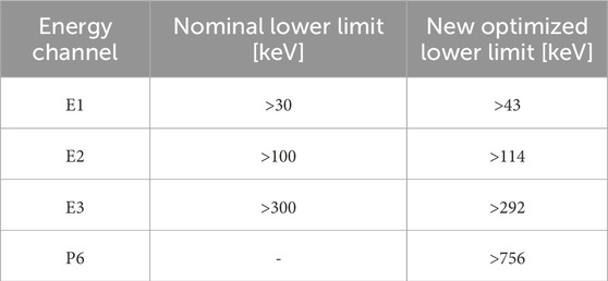
TABLE 1. Nominal detector responses in the three electron channels E1, E2, and E3 and the highest proton energy channel, P6, of the SEM-2 MEPED (Evans and Greer, 2004) and the new optimized integral energy limits for the different channels (Ødegaard et al., 2017).
The electron and proton solid-state detectors consist of a 0° and a 90° telescope. When the satellites travel across high geomagnetic latitudes, the 0° telescope will mainly measure particle fluxes that will be lost to the atmosphere. In contrast, the 90° telescope will mainly measure particles trapped in the radiation belts (Rodger et al., 2010). The energetic electron fluxes are often strongly anisotropic with decreasing fluxes towards the center of the bounce loss cone (BLC, the region where particles will be lost to the atmosphere) (Nesse Tyssøy et al., 2016). Hence, the 0° telescope will underestimate, and the 90° telescope will overestimate the precipitating electron fluxes.
Separately, the two telescopes do not accurately estimate the precipitating electron fluxes. Combining measurements from the 0° and 90° telescopes with electron pitch angle distributions from theories of wave-particle interactions in the magnetosphere, Nesse Tyssøy et al. (2016) estimated a complete BLC flux for each electron energy channel. Low-energy proton contamination is removed based on the proton telescope data. First, the proton observations are corrected for degradation due to radiation damage by applying correction factors derived by Sandanger et al. (2015) and Ødegaard et al. (2016). Subsequently, the proton flux in the energy intervals known to impact the respective electron channels (Evans and Greer, 2004) is subtracted from the originally measured electron fluxes (Nesse Tyssøy et al., 2016). The Fokker-Planck equation for electron diffusion (Kennel and Petschek, 1966; Theodoridis and Paolini, 1967) is solved for a wide range of diffusion coefficients and transformed to the satellite altitude. Taking into account the viewing directions of the telescopes relative to the magnetic field and the detector response function for different viewing angles through the detector collimator, the ratio between the fluxes detected by the 0° and 90° detector is used to identify the theoretical pitch angle distribution that best corresponds to the observations. Finally, the flux corresponding to the pitch angle range of the BLC is estimated. The size of the BLC is calculated using the International Geomagnetic Reference Field (IGRF) model. For further details on the method used to estimate the BLC fluxes, see Nesse Tyssøy et al. (2016).
This study utilizes the BLC fluxes with the new optimized effective integral limits >43, >114, >292, and >756 keV, denoted as E1, E2, E3, and P6. Figure 1 shows the coverage of the three operating NOAA satellites on the 25th of March 2004 for the Northern Hemisphere (NH) and Southern Hemisphere (SH). In the NH, data scarcity is observed around the midnight sector, corresponding to 0 magnetic local time (MLT). In the SH, the data gap is prominent around midday or 12 MLT.
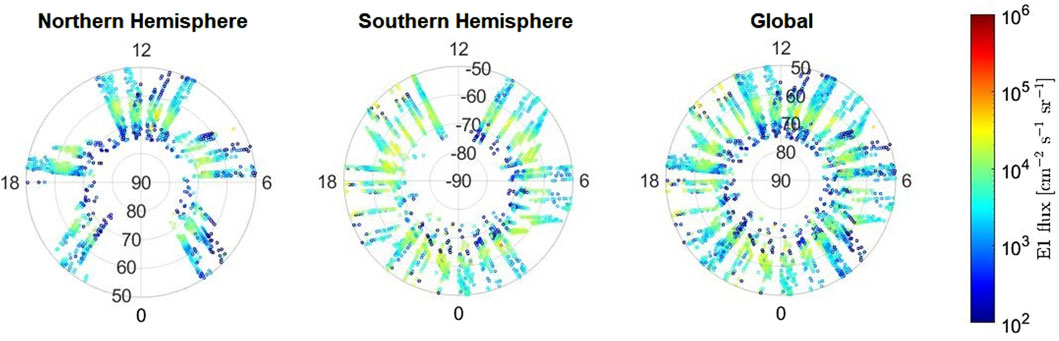
FIGURE 1. The satellite coverage of the three NOAA satellites, 15, 16, and 17, over a full day on 25 March 2004, for the Northern, Southern, and both hemispheres combined to represent a global flux. The >43 keV flux measurements for each point are indicated by the color bar.
To achieve a robust global daily average flux for 2004–2014, measurements from both hemispheres for all available MEPED data are used (see example to the right in Figure 1). This approach offers more comprehensive data points and enhanced MLT coverage. However, as different MLT sectors still have varying coverage, the daily average flux calculation is first segmented into four distinct MLT sectors: 0–6, 6–12, 12–18, and 18–24 MLT. The global daily flux is then determined by averaging the values across these four MLT sectors over the corrected geomagnetic (CGM) latitude bands: 55°–70° in the NH and −55°−70° in the SH.
During large SPEs, proton contamination dominates the counts in the MEPED electron detector, making the remaining electron fluxes after the respective proton correction uncertain (Nesse Tyssøy et al., 2016). As such, the electron fluxes with SPEs exceeding 200 particle flux units (pfu), equivalent to 200 protons cm−2s−1sr−1, have been excluded from the flux data from the SPE onset to 20°days after. The long “buffer” period after an SPE event minimizes the impact on the NO climatology and prevents SPE NO production from being misinterpreted as an EEP effect.
Overall, the BLC fluxes are an optimized estimate based on known physics and available instrumentation. Still, the pitch angle diffusion theory by Kennel and Petschek (1966) assumes steady-state conditions, which can lead to uncertainties in geomagnetic active periods (Shen et al., 2023). Moreover, a recent idealized model study by Selesnick et al. (2020) points out that the sensitivity of the 0° detector outside the nominal field of view may cause it to be susceptible to quasi-trapped or trapped electrons during periods of weak pitch angle diffusion, hence exaggerating the fluxes. Although the method applied in our study does not assume a uniform angular response, some contamination from electrons outside the nominal field of view affecting the loss cone estimates cannot be excluded.
The Solar Occultation For Ice Experiment (SOFIE) instrument onboard NASA’s Aeronomy of Ice in the Mesosphere (AIM) satellite has been measuring temperature, ice water content, and trace gases (H2O, CO2, O3, CH4, and NO) in the polar middle atmosphere since its launch in May 2007 (Gordley et al., 2009). The satellite has a polar, Sun-synchronous orbit with a period of 96 min, giving 15 orbits per day. The SOFIE instrument measures vertical NO profiles twice per orbit, one in the NH and one in the SH, during local sunset and sunrise, respectively. The latitudinal coverage depends on the time of year and varies from 65° to 85°. The vertical profiles of NO are from 30 up to 150 km with a vertical resolution of 1 km taken every 0.2 km.
During Northern Hemisphere sunrise measurements, large thermal oscillations in the SOFIE detector lead to non-retrievable NO data below 80 km [see Gómez-Ramírez et al. (2013) for further details on retrieval methods and applied corrections for the NO signal measured by SOFIE]. Additionally, sudden stratospheric warming events occur more commonly in the NH, complicating the typical polar vortex descent by bringing NO-enriched air down to the middle atmosphere. In the investigated period, no sudden stratospheric warming events occurred in the SH (Hendrickx et al., 2015). Hence, this study limits it is NO measurements to the SH, where instrument complications and sudden stratospheric warming events do not affect the NO data profiles.
This study utilizes the complete SOFIE NO data (version 1.2) publicly accessible on https://sofie.gats-inc.com/getdata, focusing on observations made over the SH from 2007 to 2014. Figure 2 presents the vertical profile of NO density, with data points provided at a daily resolution and covering an altitude range from 35 km to 150 km. One of the noteworthy features displayed in the Figure is the NO reservoir, which is consistently evident around an altitude of 100 km. This reservoir persists even during the SH’s summer months but becomes more prominent and extends further down into the atmosphere during winter. Additionally, the Figure shows an increased concentration of NO extending to an altitude of 50 km, a particularly noticeable phenomenon in the winter months.
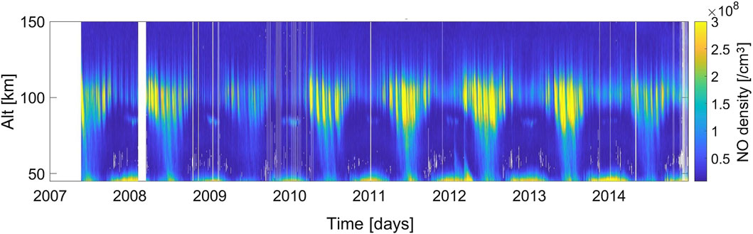
FIGURE 2. The Southern Hemisphere NO density [/cm3] data retrieved from the SOFIE instrument onboard NASA’s AIM satellite from 2007 to 2014. The data has a daily resolution from 35 to 150 km altitude.
Three primary types of solar wind flow are distinguished based on their origins from the Sun and by near-Earth solar wind parameters. Richardson and Cane (2012)’s definitions of solar wind structures are as follows:
− High-speed streams (HSSs), which originate from the Sun’s coronal holes. Solar wind speeds of v ≳ 450 km/s characterize these streams. Co-rotating interaction regions (CIR) are compressed regions between the fast streams and the preceding slower, cooler, and denser solar wind. Both the fast stream itself and the co-rotating interaction are under the term HSS.
− Transient flows connected with coronal mass ejections (CMEs). These flows comprise interplanetary CMEs (ICMEs, e.g., Kilpua et al., 2017), which are solar wind manifestations of the CMEs, as well as their associated upstream shocks and post-shock/sheath regions. CMEs, their shocks, and sheaths are collected under the term “CMEs”.
− The slower, inter-stream solar wind, typically affiliated with the Sun’s streamer belt.
This study uses an extended solar wind structure list from 2004 to 2014 based on the classification presented in Richardson and Cane (2012), and references therein).
In this study, flux peaks above the 90th percentile of the >43°keV flux are identified before being categorized by the associated absolute or relative >292 keV peak flux:
• Events with a weak or strong >292 keV peak flux are termed absolute E1 and E3 events.
• Events with a weak or strong >292 keV peak flux scaled by the >43 kev flux peak are termed relative E1 and E3 events.
Focusing on flux peaks above the 90th percentile of the >43°keV flux specifically targets the most intense events, which are often averaged out in EEP parametrizations. The aim of studying the absolute events is to identify how strong solar wind properties and geomagnetic disturbances need to be to give high >292 keV flux responses. Additionally, by examining a subset of absolute E1 and E3 events with similar/overlapping >43 keV peak fluxes, we seek to gain a deeper understanding of the specific conditions associated with acceleration and precipitation of the high-energy tail. The >292 keV peak flux correlates with the >43 keV peak flux; however, for a specific >43 keV value, the corresponding >292 keV peak flux can vary by an order of magnitude (Salice et al., 2023). Hence, exploring the relative increase between >43 and >292 keV peak fluxes allows for further insight into the conditions favorable for generating a high-energy tail, independent of the initial >43 keV flux level and total energy flux. This section will offer comprehensive details on the selection criteria for absolute, overlapping, and relative E1 and E3 events.
Figure 3 displays the global daily >43 keV (top panel) and >292 keV (bottom panel) flux data from both the Northern and Southern Hemispheres over a complete solar cycle spanning 2004 to 2014. The black lines represent the global flux values, with excluded SPEs shown in light grey. Peaks in the >43 keV electron flux exceeding the 90th percentile
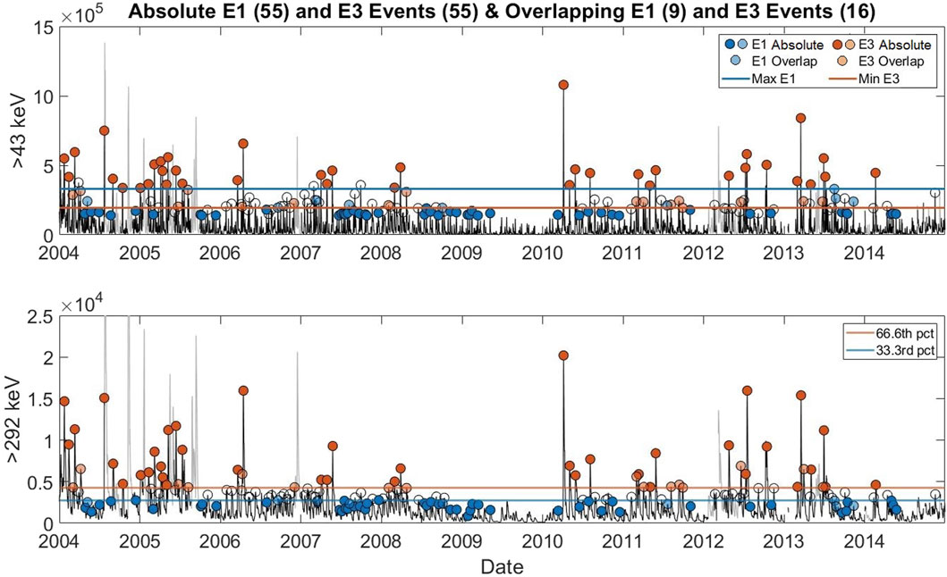
FIGURE 3. Electron fluxes for >43 keV (top) and >292 keV (bottom) energy channels from 2004 to 2014 are shown as black lines, with light grey segments indicating SPE exceeding 200 pfu. Circles mark the 164 flux peaks above the 90th percentile of >43 keV flux, with filled and subdued blue/red circles representing absolute E1/E3 events, respectively. The subset of overlapping E1 and E3 events is shown by just the subdued blue and red circles. In the bottom panel, blue and red lines indicate the 33.3rd and 66.6th percentiles of the 164 peak fluxes in the >292 keV channel corresponding to absolute E1 and E3 event thresholds. In contrast, in the top panel, the lines represent the strongest and weakest >43 keV fluxes for absolute E1 and E3 events, corresponding to overlapping E1 and E3 thresholds. Flux units are in cm−2s−1sr−1.
From the identified 164 peaks, two types of events are categorized based on the corresponding >292 keV flux peaks. Absolute E1 events comprise the third with the lowest >292 keV flux peaks, while absolute E3 events represent the third with the highest. The dividing thresholds between the events in the >292 keV flux are marked in the bottom panel: the 33.3rd percentile (blue line) at
The absolute E3 events shown in Figure 3 generally have higher >43 keV fluxes than absolute E1 events, though multiple exceptions exist. Figure 3 further distinguishes a subset of absolute E1 and E3 events with similar >43 keV fluxes, termed overlapping E1 and E3 events. This subset of overlapping events is determined by two boundaries in the >43 keV flux. The upper boundary is represented by the blue line in the top panel of Figure 3, denoting the strongest >43 keV flux peak among absolute E1 events on the 16th of August 2013 at
Note that the low number of overlapping events only provides a preliminary insight. The following discussion and conclusion will mainly rely on the more extensive dataset.
In Figure 4, as in Figure 3, the top panel displays the >43 keV flux with the 164 flux peaks above the 90th percentile as circles, both empty and filled. The middle panel mirrors this representation for the >292 keV flux. The bottom panel shows the ratio of >292 keV and >43 keV peak flux for the 164 peaks. Relative E3 events are defined as the third with the highest ratio, while relative E1 events are defined as the third with the lowest ratio. This results in 55 relative E1 and 55 relative E3 events, shown as light blue and pink circles in Figure 4, respectively.
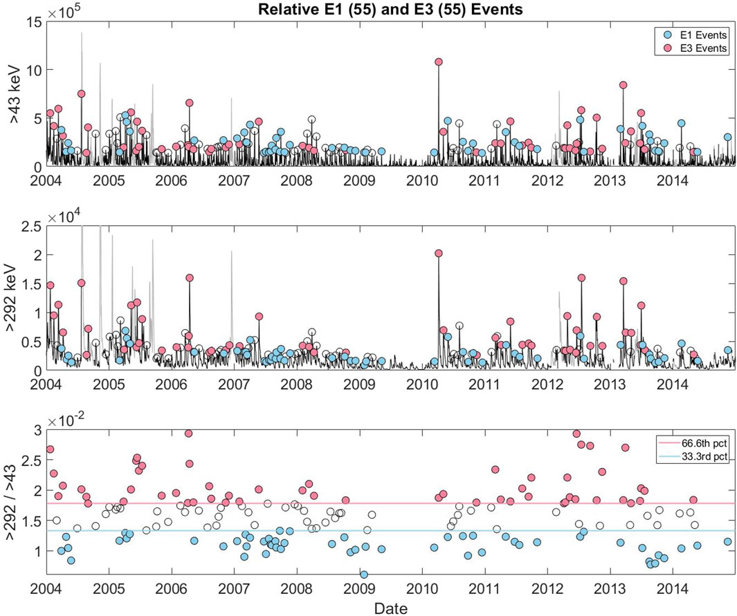
FIGURE 4. The top panel shows the >43 keV flux with circles representing the 164 flux peaks exceeding the 90th percentile. The middle panel mirrors this representation for the >292 keV flux. The bottom panel shows the ratio of >292 keV to >43 keV peak fluxes for the 164 peaks. In all panels, circles filled in light blue and pink circles denote the relative E1 and E3 events, categorized by the lowest and highest third ratios, respectively. The horizontal lines in the bottom panel mark the 33.3rd (light blue) and 66.6th (pink) percentile thresholds of the ratios. Flux units are in cm−2s−1sr−1.
Among the 110 absolute and 110 relative events, 77 are designated as both. 32 events are classified as absolute E1 and relative E1 events, meaning they have a >292 keV flux response that is both low and relatively low compared to the >43 keV flux. 32 events are classified as absolute and relative E3 events with high and relatively high >292 keV flux response. There are, in total, 13 events that are absolute E1 and relative E3 or absolute E3 and relative E1 events. A comprehensive event list is provided in the data availability section for reference.
For absolute, overlapping, and relative event peaks in the >43 keV energy channel, the dominant solar wind structure on that day and the preceding day were retrieved based on the classification described in Section 2.3. The classification follows Richardson and Cane (2012)’s definitions and list of solar wind structures from 2004 to 2014. In this study, an event is categorized as CME-driven if a CME drives either day. If neither day is a CME but at least one is an HSS, the event is classified as HSS-driven. Events not fitting these criteria are not categorized with a specific solar wind structure. The distribution of these classifications for the events is summarized in Table 2. Notably, two absolute and one relative E1 event, as well as one absolute and one relative E3 event, are not associated with any solar wind structure.
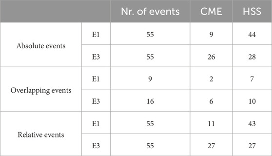
TABLE 2. Overview of the number of absolute, overlapping, and relative E1 and E3 events primarily driven by CMEs or HSSs.
Out of the 55 absolute E1 events, 44 are driven by HSSs, while only 9 are driven by CMEs. In contrast, absolute E3 events display a more balanced distribution between the two solar wind structures, with 28 driven by HSSs and 26 by CMEs. This pattern is also observed in the relative events, while the overlapping events are largely HSS-driven.
In this section, a superposed epoch analysis (SEA) for the absolute E1 and E3 events, the associated subset of overlapping E1 and E3 events, and the relative E1 and E3 events are performed. The median epoch values and the 25th and 75th percentiles are calculated for all variables. For both E1 and E3 events, the epoch time (onset) is defined as the peak in the >43 keV electron flux (see top panels of Figures 3, 4). The time ranges from 5 days before to 10 days after onset. Section 4.1 presents the SEA of the global MEE flux data and observed NO density for selected events, and Section 4.2 shows the SEA for the associated solar wind and geomagnetic data. Further, Section 4.3 sorts the selected events by their solar wind drivers, reproducing the SEA for flux response, solar wind parameters, and geomagnetic indices. Lastly, in Section 4.4, the occurrence probability of absolute E1 and E3 events for specific solar wind and geomagnetic parameters is analyzed.
Figure 5 presents a SEA of the daily flux evolution for absolute, overlapping, and relative E1 (blue/light blue) and E3 (red/pink) events across the various integral electron energy channels.
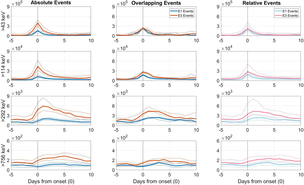
FIGURE 5. SEA of daily median electron flux evolution in various energy channels for absolute/relative E1 (blue/light blue) and E3 (red/pink) events. The left panels show the 110 absolute E1 and E3 events, the middle panels show the 25 overlapping E1 and E3 events, while the right panels display the 110 relative E1 and E3 events. Dotted lines in corresponding colors represent the 25th and 75th percentiles. The onset is the peak flux in the >43 keV electron channel for each event. Flux units are in cm−2s−1sr−1.
The left panels in Figure 5 reveal a distinct response in the >43 keV energy channel for both absolute event categories, but with the E3 events having a peak flux 2.6 times that of E1 (
As anticipated based on our selection criteria, the middle panels present the overlapping E1 and E3 events with similar peak fluxes in the >43 keV energy channel. Here, E1 and E3 events register a peak flux both at
The right panels show that the relative E1 and E3 events have similar >43 keV peak fluxes at
For all three event categories, E3 events consistently display elevated >292 keV fluxes in the days preceding the onset compared to E1 events. This suggests a higher baseline flux associated with the E3 event periods.
A noteworthy observation from Figure 5 is the temporal delay in flux peaks as energy increases, a trend evident in all three sets of panels. In particular, the peak of the high-energy tail (>292 keV) is about 1–2 days delayed compared to the >43 keV flux peak.
Figure 6 displays the temporal differences between peak fluxes in the >43 keV and >292 keV energy channels. Delays span from zero to 3 days. In this context, e.g., a 1-day delay indicates that the >292 keV peak occurs between day one and day two from onset.
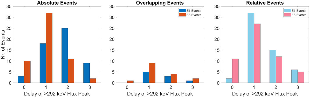
FIGURE 6. The occurrence rate of the zero-to 3-day delay in the >292 keV flux peak compared to the peak in the >43 keV flux. The absolute, overlapping, and relative categories are shown in the same sequence and colors as in Figure 5.
Most notably, 45% of absolute events (left panel) have a 1-day delay in the >292 keV flux peak relative to the >43 keV peak. Absolute E3 events predominantly display a 1-day delay (58%), whereas absolute E1 events have the highest probability of a 2-day delay (45%). A majority (76%) of absolute E3 events have short delays of up to 1 day. Comparatively, most absolute E1 events have longer delays of more than 1 day (62%).
When focusing on overlapping events (middle panel), the delay spectrum remains zero to 3 days, with both E1 and E3 events having the highest probability of a 1-day delay (both 56%). Similarly, a 1-day delay is most common for the relative E1 (58%) and E3 (49%) events shown in the right panel. Relative E3 events also exhibit a high likelihood of rapid >292 keV peak responses with 20% demonstrating a 0-day delay. Conversely, the relative E1 events tend to have longer delays as only 4% have a 0-day delay.
These findings align well with existing literature (Salice et al., 2023, and references therein), which reports a high likelihood of a 1-day delay between the >43 keV and >292 keV electron flux peaks. Salice et al. (2023) also corroborates the influence of solar wind structures on these delays, indicating shorter delays for CME-driven events and longer delays for HSS-driven events. As about 80% of the absolute and relative E1 events are associated with HSSs (see Table 2), this analysis confirms the tendency for longer delays in >292 keV fluxes for HSS-driven events.
In this subsection, we focus on variations in atmospheric nitric oxide (NO) concentrations, a crucial parameter that can further illuminate the distinct characteristics of E1 and E3 events.
Figure 7 presents a SEA of the mean SH change in NO relative to a 30-day smoothed mean baseline for each kilometer. The analysis spans altitudes from 60 to 150 km to capture NO variations throughout the mesosphere and lower thermosphere. Below 60 km, the variability in NO concentrations is influenced by dynamic atmospheric processes that can push NO to these altitudes. This fluctuating boundary layer of NO introduces noise into the data, obscuring the signals related to energetic electron precipitation, which is the focus of this study. The plots display isolated increases in NO concentration, separate from primary electron-induced enhancements; these are regarded as potential noise or phenomena unrelated to the events in question. Two dashed horizontal white lines mark the altitudes of 90 km and 70 km, which correspond to the approximate altitudes of the highest deposition rates for >43 keV and >292 keV precipitating electrons, respectively (Xu et al., 2020; Pettit et al., 2023). When analyzing the NO data, we focus on the days between 0 and 5 days from onset to identify the direct effect of EEP associated with the selected events.
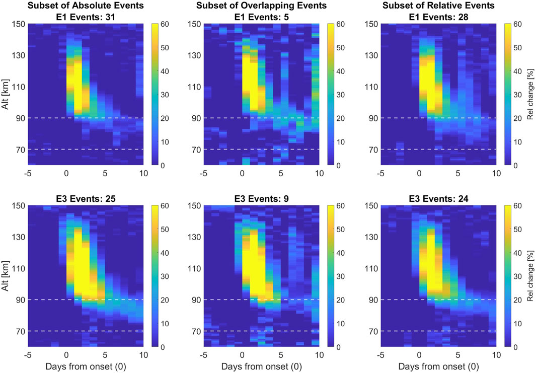
FIGURE 7. SEA comparing the daily relative increase in atmospheric NO concentrations for each category of E1 (top) and E3 (bottom) events. Data is displayed as a percentage above a 30-day smoothed mean for altitudes ranging from 60 to 150 km. The onset of events is defined consistently with Figure 5. All panels cover the time range of SOFIE measurements from May 2007 to 2014. Events with substantial missing data from onset to 4 days after are excluded. The subset of events included in each panel is indicated in their respective headings.
The left-hand panels of Figure 7 show that both absolute E1 and E3 events exhibit at least a 60% increase in NO production above 90 km altitude from the onset day to 2 days later. There are, however, notable differences. For the E3 events, the intense increase in NO production covers a broader altitude range and persists through the third day. Though subtle, absolute E3 events display a tendency for NO production directly down to 60 km at two and 3 days from onset. Direct production for absolute E1 events is only visible down to 80 km on the second day from onset. Additionally, the EEP indirect effect, visible as a descending tail in the NO density profiles from the third-day post-onset, is more pronounced in E3 events. This notable tail suggests substantial NO transport from higher altitudes where its intensity is mainly scaled to the strength of the >43 keV fluxes. Although direct production cannot be entirely excluded, the >292 keV and >756 keV fluxes are orders of magnitude lower than the >43 keV fluxes and do not align with the observed intensity or depth of the NO tail (see Figure 5).
Given the smaller sample size of overlapping events shown in the middle panels of Figure 7, the data in these panels are more susceptible to statistical fluctuations due to factors such as season and noise, making it hard to draw strong conclusions. Additionally, the wide altitude ranges of NO increase visible 5 days from onset might be caused by new geomagnetic activity. Despite these challenges, the signature characteristic of a direct EEP effect down to 60 km 2 and 3 days after onset is still evident in the overlapping E3 events, as shown in the middle bottom panel. The middle top panel shows the overlapping E1 events with hints of NO production at low altitudes between zero to 4 days from onset, though not as pronounced as for the overlapping E3 events.
In the right panels of Figure 7, both the relative E1 and E3 events are associated with direct NO production below 70 km. For the E1 events, this is visible on the second day, and for E3 events, it is visible on the second and third days from onset. It is expected that both categories of relative events show direct production at low altitudes, as it is the absolute level of direct ionization that will influence the NO production. The relative E1 events with strong >292 keV fluxes have the potential to produce NO directly below 70 km. Similarly, there will be E3 events with insufficient >292 keV to contribute to observable NO densities. This is also shown in Figure 5, where there is a overlap between percentiles in the >292 keV flux channel for relative events.
Figure 5 shows that absolute E3 events tend to exhibit higher fluxes compared to absolute E1 events. Additionally, overlapping and relative E3 events display stronger >292 keV fluxes than their E1 counterparts despite having comparable >43 keV peak fluxes. Consistent with the flux observations, Figure 7 emphasizes the distinctions between E1 and E3 events regarding NO production’s duration, intensity, and depth. Notable, absolute and overlapping E3 events have stronger NO responses reaching further down into the atmosphere over a longer time than their E1 counterparts. Both relative events show direct production down to 60 km but with the effect lasting longer for relative E3 events. In the next section, we will examine solar wind and geomagnetic data to explore the root causes of these observed disparities in Figures 5, 7 between E1 and E3 events.
To model the distinct differences found in Section 4.1 between E1 and E3 events, the daily averaged solar wind and geomagnetic data as potential predictive variables for high-energy EEP are examined. To describe the solar wind forcing, the interplanetary magnetic field (IMF) component Bz [nT] in GSM coordinates, the solar wind bulk speed v [km/s], and the epsilon parameter ϵ [GW] measuring the coupling efficiency between the IMF and the magnetosphere are used. To describe the level of geomagnetic activity, we use the ring current sensitive Dst [nT] index, the Kp*10 index measuring global geomagnetic disturbances, and the AE [nT] index, which tracks magnetic activity in the auroral regions. All indices but epsilon are retrieved from the OMNI2 (formally OMNI) database with a daily resolution from 2004–2014. Epsilon is retrieved with a minute resolution from the SuperMAG database (Gjerloev, 2012) and re-calculated to a daily average for the same period. Epsilon is given by:
The formulation of Eq. 1 draws from the work of Akasofu (1981) and is expressed in SI units (Watt) as specified by Koskinen and Tanskanen (2002). In this equation, the term 4π/μ0 = 107, v represents the solar wind velocity, B denotes the total magnetic field in the solar wind, θ is the clock angle, and l0 = 7RE. Understanding the drivers is crucial for uncovering the mechanisms responsible for the distinct characteristics of E1 and E3 events, including their varied abilities to produce NO over specific time frames and altitudes. This section presents SEAs of solar wind parameters and geomagnetic indices associated with the E1 and E3 events.
Figure 8 offers a SEA of the key solar wind parameters, Bz, v, and epsilon, where panels are organized as in Figure 5.
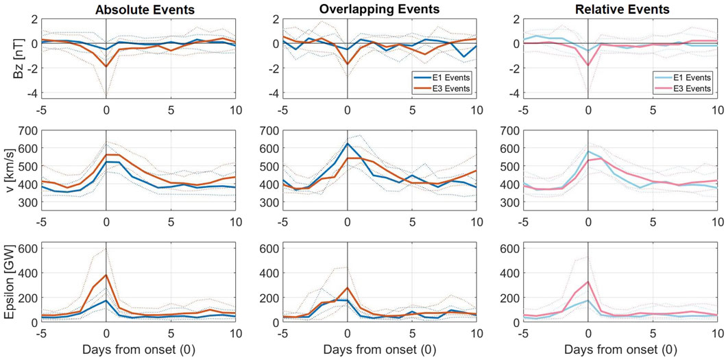
FIGURE 8. SEA of median daily solar wind properties for E1 and E3 events where the absolute, overlapping, and relative categories are shown in the same sequence and colors as in Figure 5. Solar wind properties displayed from top to bottom are the interplanetary magnetic field component in the z-direction (Bz), the solar wind bulk speed (v), and the solar wind-magnetosphere coupling function (epsilon).
The left-hand panels in Figure 8 provide insights into the behavior of the three solar wind parameters for the absolute events, which tend to be stronger for E3. More specifically, absolute E3 events have, on average, a 3.8 times stronger southward orientation of Bz and a 2.2 times higher epsilon value than absolute E1 events. However, for solar wind speed, both event types display a 2-day plateaued peak with similar values where absolute E3 events are only 1.1 times faster. Elevated responses in the solar wind parameters tend to last longer for absolute E3 events. The 3-day southward trend of Bz surpasses the 1-day tendency of absolute E1 events, indicating a more prolonged southward alignment of the interplanetary magnetic field during absolute E3 events. Additionally, absolute E3 events exhibit a slightly higher speed from several days before to 4 days after onset and elevated epsilon values from the day before to the day after onset, exceeding the duration of E1 events by 2 days.
The middle and right panels in Figure 8 examine the overlapping and relative E1 and E3 events, respectively. The Bz parameter is similar through all three panels, with only relative E3 events showing a shorter duration of the southward alignment. For solar wind speed, the overlapping and relative E1 events show almost a 1.2 and 1.1 times stronger tendency, respectively, than the speed for the corresponding E3 events. However, overlapping and relative E3 events typically demonstrate a delayed peak or sustained elevation in solar wind speed 1 day post-onset, followed by a more gradual recovery than their E1 counterparts. This time shift and prolonged impact for overlapping and relative E3 events is not evident for absolute events. The epsilon parameter for the relative events resembles that of absolute events, though with slightly weaker responses in the relative E3 events. For overlapping events, however, the responses between E1 and E3 are similar for the 2 days pre-onset. The overlapping E3 events still have tendencies for a higher energy transfer from onset to 1 day after.
The intersecting percentiles in the plots indicate that E1 and E3 events can have similar solar wind driving factors. Hence, the median values suggest probable differences rather than absolute distinctions.
Figure 9 adopts the same layout and time-window structure as Figure 8 but focuses on the key geomagnetic indices Dst, Kp*10, and AE. For absolute events, the geomagnetic indices Dst, Kp*10, and AE consistently show stronger peak/trough responses during E3 events compared to E1. The average minimum Dst response for the E3 events reaches 2.4 times deeper than for E1 events, emphasizing the most significant variance among the indices. The Kp*10 and AE peaks for absolute E3 events are 1.3 and 1.6 times those of E1 events, respectively. The more intense geomagnetic deflections highlight the stronger geomagnetic activity associated with absolute E3 events. On the day before onset, a pronounced divergence between the events is visible, with absolute E3 events consistently registering stronger responses. This difference continues post-onset, where Kp*10 and AE return to comparable levels about 4 days later and Dst takes even longer.
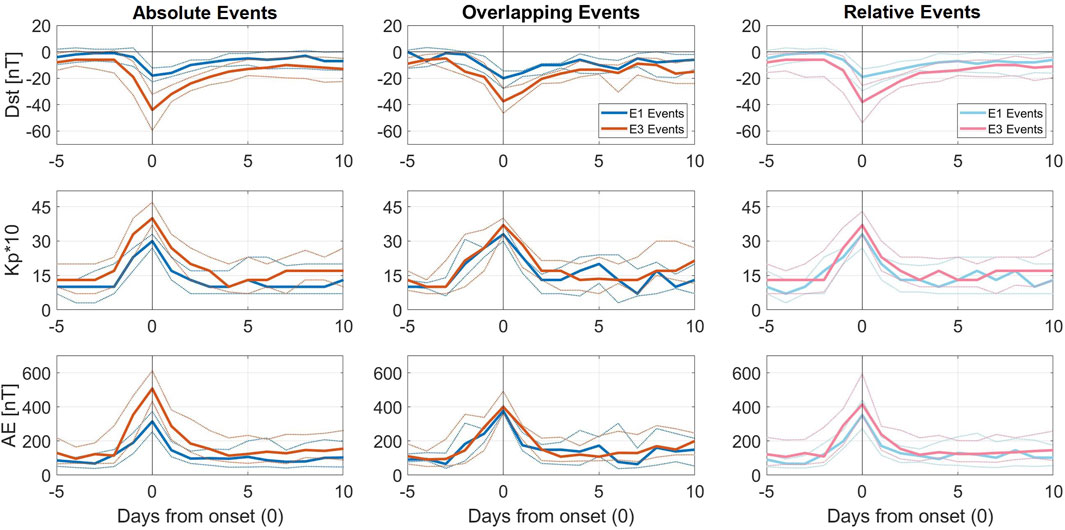
FIGURE 9. The same as in Figure 8 just for geomagnetic indices. From top to bottom, the Dst, Kp*10, and AE indices are shown.
For the overlapping (middle panels) and relative (right panels) events, the differences in Kp*10 and AE converge, with E3 responses being less than 1.2 times higher with a large percentile overlap. The differences in Dst, however, remain; overlapping and relative E3 events show a minimum that is twice as strong as E1 events, with less percentile overlap compared to the other indices. Overlapping and relative E3 events tend to show stronger responses post-onset (2–4 days) across all indices and pre-onset (2–3 days) for Dst. Notably, relative E3 events also exhibit increased AE activity pre-onset compared to E1.
Although not depicted, the pressure-corrected Dst index and the RC index—derived from the Dst index and previously demonstrated to offer a more accurate portrayal of global geomagnetic variations than Dst (Olsen et al., 2014)—were also subjected to SEAs. However, the outcomes from this analysis did not reveal any notable distinctions from those obtained using Dst. Similarly, an evaluation of the substorm rate, known to correlate strongly with the AE index, did not yield additional insights when analyzed in this manner.
In examining key solar wind and geomagnetic parameters, no single parameter can distinguish between E1 and E3 events. However, distinctive patterns emerge. Dst is the only geomagnetic index showing potential for distinguishing between E1 and E3 events across all categories. This indicates that Dst might be best linked to the variations in the >292 keV flux. Stronger southward Bz orientations and heightened epsilon responses over longer times also tend to be characteristic of all types of E3 events. Only solar wind speed exhibits a distinct pattern between the overlapping/relative and absolute events.
This subsection presents SEAs of MEE fluxes, solar wind, and geomagnetic indices, including the categorization of E1 and E3 events by their specific solar wind structure, HSS, or CME. The aim is to identify whether the discrepancies between E1 and E3 events are influenced by their respective solar wind structure as listed in Table 2. Note that the respective separation results in a very weak statistic for the overlapping events. Hence, the resulting SEAs are shown only for completeness, but potential findings regarding overlapping events are disregarded in the text.
Figure 10 shows the precipitating MEE fluxes as in Figure 5 but with the E1 and E3 events separated into HSSs and CMEs. In general, the difference between absolute E1 and E3 events is still prominent, as shown in the left panels of Figure 5. The HSS- (light blue) and CME-driven (blue) absolute E1 events show similar flux levels in all energy channels. The absolute E3 events, however, show visible differences where the fluxes associated with CMEs (red) are higher than those associated with HSSs (orange). The relative CME-driven E3 events have higher flux responses in all channels than HSS-driven E3 events (right panels). This includes the >43 keV channel where in Figure 5, all average flux peaks were the same.
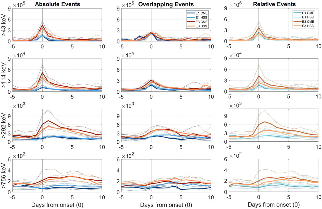
FIGURE 10. The same as Figure 5 but with events separated into solar wind drivers. For the absolute and overlapping E1 and E3 events, CMEs are in blue and red, and HSSs are in light blue and orange, respectively. Relative events are in similar offset colors. Note that the >292 keV flux channel is on a different scale than in Figure 5.
Figure 11 presents the same solar wind properties as in Figure 8 but with the E1 and E3 events separated into HSS- or CME-driven as in Figure 10. CME-driven events have larger Bz and epsilon deflections than their HSS-driven counterparts. An exception occurs in the solar wind speed, where the opposite is true.
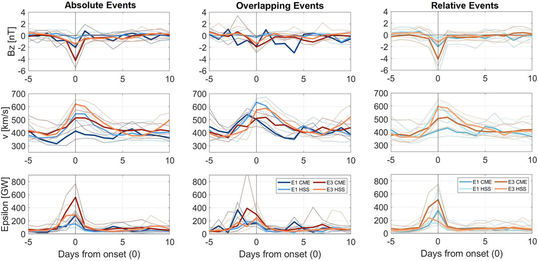
FIGURE 11. The same as Figure 8 but with E1 and E3 events separated into solar wind drivers as in Figure 10. Note that Bz and Epsilon are on a different scale than in Figure 8.
The absolute events in the left panels of Figure 11 show that CME-driven absolute E1 (blue) and HSS-driven absolute E3 (orange) events have the same peak responses in Bz and epsilon, but the HSS-driven E3 events last longer with a broader peak. However, the differences between CME-driven E3 (red) and HSS-driven E1 (light blue) events are substantial for these parameters. For solar wind speed, it is the opposite. The CME-driven E1 events and HSS-driven E3 events are associated with the lowest and highest solar wind speeds, respectively. The CME-driven E3 events and HSS-driven E1 events have similar speed levels. It demonstrates that the overlapping percentiles in Figure 8 can largely be ascribed to different solar wind drivers.
The solar wind parameters for the relative E1 and E3 events in the right panels resemble the absolute events, demonstrating that it is the CME-driven E1 events and HSS-driven E3 events that are responsible for the overlap between the event types in Bz and epsilon. For all solar wind parameters, the HSS-driven E1 and E3 events converge, giving the weakest responses in Bz and epsilon and the strongest in solar wind speed. Delayed or prolonged solar wind speeds following onset are evident for both the CME- and HSS-driven relative E3 events.
In Figure 12, the geomagnetic indices are portrayed in the same manner as in Figure 9, and the events are separated into solar wind drivers as in Figures 10, 11.
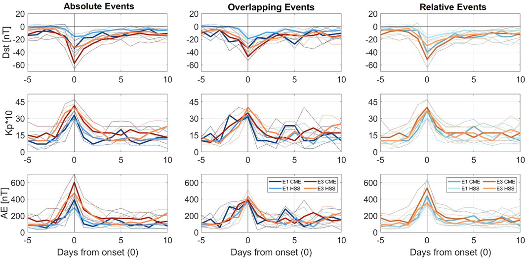
FIGURE 12. The same as in Figure 9 separated into solar wind drivers in the same way as in Figures 10, 11.
The absolute events in the left panels of Figure 12 show that Dst has clear structure-dependent variations. CME-driven E1 (blue) and HSS-driven E3 (orange) events have similar Dst troughs, but the HSS-driven E3 events show a longer recovery time. The largest differences are between CME-driven E3 (red) and HSS-driven E1 (light blue) events. Kp*10 and AE show no dependency on structure, with the absolute E3 events having stronger responses than E1 events independent of the solar wind driver. However, tendencies for stronger and sharper responses for the CME-driven events compared to the HSS-driven ones are evident.
The relative events in the right panels of Figure 12 show that the CME-driven E1 and E3 events tend to have stronger responses than the HSS-driven ones in Dst and AE. In Kp*10, all but the HSS-driven E1 events show the same peak response.
In summary, as shown in Figures 8, 9, there is a significant overlap between the percentiles of E1 and E3 events. Based on the findings in Figures 11, 12, some of this percentile overlap can be ascribed to solar wind structures, as a clearer separation of E1 and E3 events is possible if the solar wind structure is known. The Dst index especially exhibits pronounced structure-dependent variations among E1 and E3 events. It suggests that knowing the underlying solar wind structure is crucial for establishing specific thresholds for the occurrence of E3 events.
The absolute events allow a general assessment of which geomagnetic deflections or solar wind parameters are associated with high and low >292 keV fluxes. This subsection explores the predictive probability of the solar wind parameters and geomagnetic indices with respect to the occurrence of absolute E1 or E3 events, as depicted in the top panels of Figure 13. These panels illustrate the occurrence probabilities for the 55 absolute E1 events (blue) and the 55 absolute E3 events (red) based on the largest daily average values of epsilon, Dst, and Kp*10, observed from 2 days before to 2 days after the event onset. Moreover, the probabilities for events driven by CMEs and HSSs are shown with dashed lines in darker and lighter shades of the corresponding colors, respectively. The bottom panels of the figure present the number of events included in each bin. For the epsilon parameter, the bins are segmented in 200 GW increments, ranging from 0 to 4,600 GW. It is important to note that the plot does not include three E3 events with peak epsilon values of 1,900, 2,700, and 4,500 GW, as the x-axis extends only up to 1,700 GW. For Dst and Kp*10, the bins are set at intervals of 10 nT and 5, with ranges from −110 to 0 nT and 20 to 75, respectively.
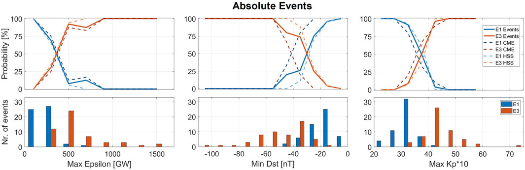
FIGURE 13. Probability of absolute E1 (blue) and E3 (red) event occurrence based on the largest daily average values of epsilon, Dst, and Kp*10 (top panels). Events driven by CMEs and HSSs are differentiated with dashed lines in darker and lighter corresponding colors, respectively. The lower panels show the distribution of events within each bin.
The three panels of Figure 13 identify distinct thresholds at which the probability of absolute E1 or E3 event diverges. For epsilon, Dst, and Kp*10, this divergence occurs at approximately 400 GW, −30 nT, and 35, respectively. Beyond these points, the likelihood of an E3 event increases with greater geomagnetic activity and the likelihood of an E1 event with weaker. Furthermore, there are specific value ranges where the analysis guarantees or excludes an event with >95% probability: epsilon values below 200 GW, Dst values above −20 nT, and Kp*10 values below 30 will almost certainly correspond to an E1 event, while for an E3 event, the corresponding thresholds are epsilon values above 700 GW, Dst below −50 nT, and Kp*10 above 40. For epsilon, Dst, and Kp*10, 36%, 52%, and 55% of the events are within these high-probability ranges, respectively. The events not included in these ranges vary slightly for the different parameters. Hence, applying more than one index could lead to fewer events falling in the high-uncertainty region.
When analyzing the events sorted by their solar wind drivers, as indicated by the dashed lines, the divergence threshold in Dst exhibits notable variation. For events driven by HSSs, the threshold slightly shifts, only a few nT above the non-separated event threshold. In contrast, for CME-driven events, the divergence threshold shifts to around −40 nT, presenting a 10 nT discrepancy from the combined event analysis. Furthermore, with the solar wind structure known, Dst can, with >95% certainty, account for up to 65% of the 110 absolute events. If CME-driven, the high probability threshold shifts from −50 to −45 nT, and if HSS-driven, it shifts from −20 to −25 nT. In the case of epsilon and Kp*10, however, a clear separation based on different solar wind structures is not as evident.
The Bz, v, and AE parameters were subjected to the same probabilistic analysis as in Figure 13. Bz did not yield significant insights, as its short range of daily averaged values could not meaningfully differentiate between E1 and E3 events. AE demonstrated trends similar to Kp*10 but with a larger range of values that could correspond to both E1 and E3 events. The solar wind speed presented a broad spectrum of values that could correspond to both events, indicating significant overlap. Notably, the distinction between solar wind drivers increased the prediction quality but was not comparable to the shown parameters epsilon, Dst, and Kp.
This subsection investigated the occurrence probability of absolute E1 and E3 events, revealing that for peak values of epsilon, Dst, and Kp*10, there are thresholds in which one becomes more likely than the other. Additionally, there are specific threshold values that can almost ensure the classification of E1 or E3 events. Based on the 110 absolute events, 36% for epsilon, 52% for Dst, and 55% for Kp*10 are within this high probability range. However, when solar wind structure is considered, Dst is the only index that increases its accuracy to include 65% of events in the high probability range.
The overarching objective of this study is to unravel the characteristics of solar wind properties and geomagnetic indices associated with the high-energy tail of MEE precipitation, enabling a better parameterization of the full energy range of EEP. This implies a parameterization that can determine the true range of flux variability, not averaging out strong events as demonstrated in Nesse Tyssøy et al. (2022) and Sinnhuber et al. (2022). Such parameterization will allow for an understanding of the importance of EEP’s direct effect on the lower mesosphere and upper stratosphere chemistry, which further affects both the strength and timing of the subsequent impact on atmospheric dynamics.
From the 164 flux peaks exceeding the 90th percentile of the >43 keV flux, absolute and relative E1 and E3 events are defined based on the absolute >292 keV flux and the ratio of >292 keV and >43 keV fluxes, respectively. The absolute events allow a general assessment of which geomagnetic deflections or solar wind parameters are associated with high and low >292 keV fluxes. Moreover, the relative events allow for the investigation of favorable conditions for enhanced >292 keV fluxes, independent of the >43 keV response. The latter also applies to the subset of absolute events with overlapping >43 keV fluxes. These distinctions are further established through SEAs of NO observations, confirming both direct and indirect effects on NO density, with a notable direct impact in the lower mesosphere predominantly associated with absolute E3 events (see Figure 7).
The solar wind fuels the energy driving the magnetospheric processes that increase the population of high-energy tail electrons (≳ 300 keV) and subsequently scatter them into the loss cone. A southward IMF (negative Bz) induces a large-scale electric field that transports electrons from the magnetotail into the inner magnetosphere, where they become part of the electron source population in the plasmasheet. Fast solar wind speed has been considered one of the most important predictors for transporting fluxes of the electron source population from the plasmasheet to the radiation belt region, trapping ≳ 300 keV electrons in the inner magnetosphere (Katsavrias et al., 2021; Stepanov et al., 2021). Combined, Bz and solar wind speed can be used to estimate the bulk energy transfer from the solar wind into the magnetosphere via dayside reconnection rate by applying coupling functions such as the widely used epsilon parameter by Akasofu (1981).
Figure 8 confirms that all three types of E3 events tend to have a stronger southward IMF component and stronger energy transfer into the magnetosphere compared to E1 events. How much energy is required to guarantee an absolute E3 event is, however, more uncertain. Figure 13 shows that for epsilon peak values above 700 GW and below 200 GW, there is >95% probability of an E3 and E1 event, respectively. These thresholds result in an uncertainty range of 500 GW, encompassing 64% of the identified events. Salice et al. (2023) explored the same daily precipitation fluxes in the NH and found that the epsilon coupling function accumulated over 4 days correlates well (0.84) with the >292 keV peak flux. Figure 4 in Salice et al. (2023) shows, however, that the spread in potential flux responses is typically about an order of magnitude, consistent with the wide band of epsilon values corresponding to absolute E1 and E3 events.
Moreover, the overlapping and relative events where similar levels of >43 keV fluxes result in very different high-energy tail fluxes confirm that neither Bz, solar wind speed, nor epsilon alone can predict the occurrence of high-energy tail precipitation. Figure 8 shows that solar wind speed tends to be similar for E1 and E3 events. However, the elevated (>500 km/s) plateau in the solar wind speed for overlapping and relative E3 events starts at the onset, 1 day after that of E1 events, and declines slower, implying higher speeds in the recovery phase of the storm. Figure 11 shows that E1 and E3 events driven by CMEs, in general, are associated with lower speed compared to E1 and E3 events driven by HSSs. However, for relative events, both CME- and HSS-driven E3 events show high speeds 1 day after onset with a gradual recovery. This suggests that the timing and/or duration of elevated solar wind speed is a potential factor for driving the high-energy tail of MEE precipitation by providing a persistent magnetospheric acceleration mechanism after the flux rise of the ≳ 30 keV electron source population.
The energy transfer to the magnetosphere from the solar wind is dissipated into three main sinks: Joule heating, auroral particle precipitation, and ring current injection (e.g., Tenfjord and Østgaard, 2013). The magnetospheric energy loss to Joule heating and auroral particle precipitation typically occurs in the main phase of a strong geomagnetic disturbance, while the ring current energy is “temporarily stored” in the magnetosphere. Assuming that the AE index represents energy dissipation of Joule heating and auroral particle precipitation and the Dst index the ring current growth, Figure 9 confirms that more energy is dissipated into the ring current during E3 events, compared to E1 events. In fact, for relative and overlapping events, the AE and Kp*10 values converge while the Dst remains notably deflected for E3 events compared to E1 events. This suggests a larger build-up of ring current particles associated with both absolute and relative E3 events.
The subsequent decay of the ring current is caused by several particle loss processes, such as scattering by Coulomb collisions, charge exchange, wave-particle interactions, and convection transporting the ions across the magnetopause (Søraas et al., 2004). The ring current decay begins when Bz turns less southward as the large-scale convection electric field will no longer transport particles to the inner magnetosphere (Jaynes et al., 2015). This is clear in the SEAs shown for Bz and Dst in Figures 8, 9, respectively. After the typical fast initial decay, the decay becomes more gradual depending on the charge exchange between the ring current ions and the geocorona as well as wave-particle interaction at or near the plasmapause forcing particles into the atmospheric loss cone (Søraas et al., 1999). The loss processes result in a ring current decay time of about 7–10 h (Søraas et al., 2004).
Based on Figure 6, the >292 keV flux peak typically occurs one and 2 days after the zero epoch. This delay corresponds to the strongest positive gradient of Dst after its deep minima on the zero epoch day. As such, there might be a physical link between the Dst recovery phase and MEE precipitation, including the high-energy tail. This would, however, require elevated substorm occurrence rates in the storm recovery phase to generate chorus waves that will scatter the ring current electrons into the loss cone. The respective chorus waves will simultaneously be responsible for electron loss in the MEE range in the radiation belts. Notably, Newell et al. (2016) demonstrated a close link between substorm probabilities and solar wind speed, reinforcing the earlier suggestion that elevated solar wind speeds in the recovery phase of a storm contribute to high >292 keV fluxes.
The Auroral Electrojet (AE) index is also found to be well correlated to the substorm occurrence rate on a daily scale (Tyssøy et al., 2021). From the SEA in Figure 9, all three categories of E3 events are associated with a higher AE response in the recovery phase of the Dst than E1 events. A higher substorm onset rate for E3 events is confirmed by examining the daily average from the substorm list provided by the number of substorms per day based on Newell and Gjerloev (2011). There is, however, not a significant difference across all categories of events. Tyssøy et al. (2021) created an AE-based MEE proxy by accumulating the AE activity over multiple days, including terms counting for the associated lifetimes. The results showed that AE-based proxies can predict at least 70% of the observed MEE precipitation variance at all energies. Applying the AE-based model to our events does capture the general features of our SEA flux analysis. It is, however, not able to identify the individual E3 events. Hence, a higher substorm onset rate in the recovery phase alone does not appear to be exclusively able to explain the high-energy tail of MEE precipitation found for E3 events.
Kp has been found to correlate well with >30 keV EEP and is commonly used in models due to its availability and long existence, e.g., as in van de Kamp et al. (2016), van de Kamp et al. (2018)’s model. The probability assessment presented in Figure 13 revealed Kp*10 as one of the best parameters independent of the solar structure as it can exclude or guarantee 55% of absolute E1 and E3 events. However, as shown in Figures 9, 12, Kp*10 is less effective in differentiating between overlapping and relative E1 and E3 events with similar >43 keV peak fluxes.
Figure 13 reveals the effectiveness of Dst in predicting up to 65% of events when the solar wind structure is considered. It has long been known that Dst has different characteristics for HSSs and CMEs (Borovsky and Steinberg, 2006). For CME-driven events, E1 or E3 events can be determined or excluded with 95% probability above −25 and below −50 nT. For HSS-driven events, these thresholds are above −20 and below −45 nT. The latter nominates the Dst index to most accurately predict if a specific geomagnetic disturbance will lead to a large MEE precipitation response in the >292 keV channel. If combined with consideration of the timing and/or duration of elevated solar wind speed in the recovery phase of the storms, there is a potential for even better prediction capabilities and an understanding of the physical mechanisms responsible for the high-energy tail of the MEE precipitation in the atmosphere. To fully examine if a specific storm will generate high-energy MEE precipitation requires case studies, which is beyond the scope of the current paper.
The overarching objective of this study is to explore and better understand the high-energy tail of MEE precipitation in the context of solar wind properties and geomagnetic responses. The research contributes to refining EEP parameterization by offering insights into the high-energy tail that can be used to improve the accuracy of the full energy range of EEP parameterization in chemistry-climate models. The electron flux data is retrieved from MEPED aboard the POES/Metop satellite series over an entire solar cycle from 2004 to 2014.164 peaks in the >43 keV electron flux exceeding the 90th percentile are categorized into absolute, overlapping, and relative E1 and E3 events. This selection of events allows for a concentrated study on intense electron flux occurrences, addressing a gap in current understanding and limitations.
Of the 164 peaks, absolute E1 and E3 events are defined by the third highest and lowest peaks in the >292 keV flux, respectively. Overlapping events, sharing similar >43 keV peak responses, were also identified, though their low number necessitates cautious interpretation. Moreover, relative E1 and E3 events are defined as the third with the lowest and highest ratio between >292 keV and >43 keV flux peaks, respectively. Overlapping and relative events provide insight into which conditions generate a high-energy tail independent of the initial ≳ 30 keV flux level. Observations of the NO density estimated from the SOFIE instrument on board the AIM satellite confirm that absolute E3 events will directly impact the lower mesosphere, which motivates the need to parameterize the full range of EEP.
Based on our SEAs, no single solar wind nor geomagnetic parameter captures the differences between E1 and E3 events across the absolute, overlapping, and relative categories. However, tendencies are visible, allowing us to suggest the following hypothesis.
The high-energy tail (≳ 300 keV) of electron precipitation requires an increased source population (≳ 30 keV) in the main phase of the storm. These ≳ 30 keV electrons will first be accelerated and then precipitate into the atmosphere or contribute to the ring current and radiation belt populations. A sustained elevation in solar wind speed during the recovery phase of a storm increases the substorm onset rate, which ensures electron acceleration to high energies and subsequent scattering into the loss cone from both the ring current and radiation belts. Hence, overlapping and relative E3 events are likely associated with elevated solar wind speeds persisting in the recovery phase of a deep Dst trough. The magnetospheric processes that accelerate and scatter electrons in the recovery phase of a storm further explain the delay often found in the >292 keV peak compared to the >43 keV peak.
As single predictors for absolute E1 or E3 events, epsilon is the best solar wind parameter, and Dst and Kp*10 are the best geomagnetic indices. Each of the three variables has a specific threshold where the probability of an E3 (E1) event becomes more likely with increasing (decreasing) activity. For epsilon, Dst, and Kp*10, the thresholds are at 400 GW, −30 nT, and 35,respectively.
Furthermore, Dst and Kp*10 have defined thresholds where the probability of either an absolute E1 or E3 event occurring is >95%, accounting for over half of the events. Specifically, 52% of absolute events fall within this high-probability range for Dst and 55% for Kp*10. The thresholds for an E1 event are for Dst values above −20 nT and Kp*10 values below 30. For E3 events they are for Dst values below −50 nT and Kp*10 values above 40.
Solar wind speed and the Dst index exhibit pronounced structure-dependent variations compared to other parameters. Knowledge of the solar wind structure confines the high probability limits, increasing Dst’s predictive accuracy to 65%. The 35% of events within the ambiguous range of Dst values might be determined by examining solar wind speed. Future studies will focus on case studies to explore the high-energy tail response in relation to elevated solar wind speed and the Dst recovery phase.
The original contributions presented in the study are included in the article/Supplementary Material, further inquiries can be directed to the corresponding author. The NOAA/POES MEPED data used in this study are available from the National Oceanic and Atmospheric Administration (https://www.ngdc.noaa.gov/stp/satellite/poes/dataaccess.html). The bounce loss cone fluxes used in this study are available at Zenodo via https://doi.org/10.5281/zenodo.6590387. Geomagnetic indices and solar wind parameters were obtained from NASA Omniweb at https://omniweb.gsfc.nasa.gov/form/dx1.html. We gratefully acknowledge the SuperMAG collaborators (https://supermag.jhuapl.edu/info/?page=acknowledgement) where the epsilon parameter was downloaded. The AIM-SOFIE data (version 1.2) are found online at https://sofie.gats-inc.com/getdata.
JS: Writing–original draft, Writing–review and editing. HN: Supervision, Writing–original draft, Writing–review and editing. NP: Writing–review and editing. EK: Writing–review and editing. AK: Writing–review and editing. MD: Writing–review and editing. EB: Writing–review and editing. CS-J: Writing–review and editing.
The author(s) declare that financial support was received for the research, authorship, and/or publication of this article. The study is supported by the Norwegian Research Council (NRC) under contracts 223252 and 302040.
HN further acknowledges the Young CAS (Centre for Advanced Studies) fellow program. EK acknowledges the Finnish Centre of Excellence in Research of Sustainable Space, Project 1336807, for supporting this research. The authors thank NOAA for providing the MEPED data, OMNIWeb for solar wind and geomagnetic data, and the AIM mission for providing SOFIE data. The authors thank Ian G. Richardson for providing the list of solar wind classifications.
The authors declare that the research was conducted in the absence of any commercial or financial relationships that could be construed as a potential conflict of interest.
All claims expressed in this article are solely those of the authors and do not necessarily represent those of their affiliated organizations, or those of the publisher, the editors and the reviewers. Any product that may be evaluated in this article, or claim that may be made by its manufacturer, is not guaranteed or endorsed by the publisher.
The Supplementary Material for this article can be found online at: https://www.frontiersin.org/articles/10.3389/fspas.2024.1352020/full#supplementary-material
SUPPLEMENTARY TABLE S1Overview of the dates for the >43 keV peaks for absolute (left-hand side) and relative (right-hand side) E1 and E3 events. ‘∗’ indicates the subset of absolute events that are also overlapping events. Purple dates indicate that the event is CME-driven, while those without color are HSS-driven. The events marked with a “!” are not associated with a solar wind structure. Bold dates, both black and purple, show the events that are both in the absolute data set and in the relative data set. Dates that are in both datasets but in different categories, e.g., absolute E1 and relative E3 or absolute E3 and relative E1, are bold and italic.
Akasofu, S. I. (1981). Energy coupling between the solar wind and the magnetosphere. Space Sci. Rev. 28. doi:10.1007/BF00218810
Angelopoulos, V., Zhang, X.-J., Artemyev, A. V., Mourenas, D., Tsai, E., Wilkins, C., et al. (2023). Th: energetic electron precipitation driven by electromagnetic ion cyclotron waves from ELFIN’s low altitude perspective. Space Sci. Rev. 219, 37. doi:10.1007/s11214-023-00984-w
Asikainen, T., and Ruopsa, M. (2016). Solar wind drivers of energetic electron precipitation. J. Geophys. Res. Space Phys. 121, 2209–2225. doi:10.1002/2015JA022215
Babu, E. M., Nesse, H., Hatch, S. M., Olsen, N., Salice, J. A., and Richardson, I. G. (2023). An updated geomagnetic index-based model for determining the latitudinal extent of energetic electron precipitation. J. Geophys. Res. Space Phys. 128. doi:10.1029/2023JA031371
Babu, E. M., Tyssøy, H. N., Smith-Johnsen, C., Maliniemi, V., Salice, J. A., Millan, R. M., et al. (2022). Determining latitudinal extent of energetic electron precipitation using MEPED on-board NOAA/POES. J. Geophys. Res. Space Phys. 127. doi:10.1029/2022JA030489
Baldwin, M. P., and Dunkerton, T. J. (2001). Stratospheric harbingers of anomalous weather regimes. Science 294, 581–584. doi:10.1126/science.1063315
Beharrell, M. J., Honary, F., Rodger, C. J., and Clilverd, M. A. (2015). Substorm-induced energetic electron precipitation: morphology and prediction. J. Geophys. Res. Space Phys. 120, 2993–3008. doi:10.1002/2014JA020632
Borovsky, J. E., and Steinberg, J. T. (2006). The “calm before the storm” in CIR/magnetosphere interactions: occurrence statistics, solar wind statistics, and magnetospheric preconditioning. J. Geophys. Res. Space Phys. 111. doi:10.1029/2005JA011397
Clilverd, M. A., Seppälä, A., Rodger, C. J., Mlynczak, M. G., and Kozyra, J. U. (2009). Additional stratospheric NOx production by relativistic electron precipitation during the 2004 spring NOx descent event. J. Geophys. Res. Space Phys. 114. doi:10.1029/2008JA013472
Daae, M., Espy, P., Nesse Tyssøy, H., Newnham, D., Stadsnes, J., and Søraas, F. (2012). The effect of energetic electron precipitation on middle mesospheric night-time ozone during and after a moderate geomagnetic storm. Geophys. Res. Lett. 39. doi:10.1029/2012GL053787
Damiani, A., Funke, B., López Puertas, M., Santee, M. L., Cordero, R. R., and Watanabe, S. (2016). Energetic particle precipitation: a major driver of the ozone budget in the Antarctic upper stratosphere. Geophys. Res. Lett. 43, 3554–3562. doi:10.1002/2016GL068279
Duderstadt, K. A., Huang, C.-L., Spence, H. E., Smith, S., Blake, J. B., Crew, A. B., et al. (2021). Estimating the impacts of radiation belt electrons on atmospheric chemistry using FIREBIRD II and van allen probes observations. J. Geophys. Res. Atmos. 126. doi:10.1029/2020JD033098
Evans, D. S., and Greer, M. S. (2004). Polar orbiting environmental satellite Space environment monitor - 2: instrument descriptions and archive data documentation, NOAA technical memorandum version 1.4.
Funke, B., Baumgaertner, A., Calisto, M., Egorova, T., Jackman, C. H., Kieser, J., et al. (2011). Composition changes after the Halloween solar proton event: the High Energy Particle Precipitation in the Atmosphere (HEPPA) model versus MIPAS data intercomparison study. Atmos. Chem. Phys. 11, 9089–9139. doi:10.5194/acp-11-9089-2011
Funke, B., Dudok de Wit, T., Ermolli, I., Haberreiter, M., Kinnison, D., Marsh, D., et al. (2023). Towards the definition of a solar forcing dataset for CMIP7. Geosci. Model Dev. Discuss. 2023, 1–14. doi:10.5194/gmd-2023-100
Gjerloev, J. W. (2012). The SuperMAG data processing technique. J. Geophys. Res. 117. doi:10.1029/2012JA017683
Gómez-Ramírez, D., McNabb, J. W. C., Russell, J. M., Hervig, M. E., Deaver, L. E., Paxton, G., et al. (2013). Empirical correction of thermal responses in the Solar Occultation for Ice Experiment nitric oxide measurements and initial data validation results. Appl. Opt. 52, 2950–2959. doi:10.1364/AO.52.002950
Gordley, L. L., Hervig, M. E., Fish, C., Russell, J. M., Bailey, S., Cook, J., et al. (2009). The solar occultation for ice experiment. J. Atmos. Solar-Terrestrial Phys. 71, 300–315. doi:10.1016/j.jastp.2008.07.012
Hendrickx, K., Megner, L., Gumbel, J., Siskind, D. E., Orsolini, Y. J., Tyssøy, H. N., et al. (2015). Observation of 27-day solar cycles in the production and mesospheric descent of EPP-produced NO. J. Geophys. Res. Space Phys. 120, 8978–8988. doi:10.1002/2015JA021441
Jackman, C. H., DeLand, M. T., Labow, G. J., Fleming, E. L., Weisenstein, D. K., Ko, M. K. W., et al. (2005). Neutral atmospheric influences of the solar proton events in October–November 2003. J. Geophys. Res. Space Phys. 110. doi:10.1029/2004JA010888
Jaynes, A. N., Baker, D. N., Singer, H. J., Rodriguez, J. V., Loto’aniu, T. M., Ali, A. F., et al. (2015). Source and seed populations for relativistic electrons: their roles in radiation belt changes. J. Geophys. Res. Space Phys. 120, 7240–7254. doi:10.1002/2015JA021234
Katsavrias, C., Aminalragia–Giamini, S., Papadimitriou, C., Sandberg, I., Jiggens, P., Daglis, I., et al. (2021). On the interplanetary parameter schemes which drive the variability of the source/seed electron population at GEO. J. Geophys. Res. Space Phys. 126, e2020JA028939. doi:10.1029/2020JA028939
Kennel, C. F., and Petschek, H. E. (1966). Limit on stably trapped particle fluxes. J. Geophys. Res. 71, 1–28. doi:10.1029/JZ071i001p00001
Khazanov, G. V., and Glocer, A. (2020). How magnetically conjugate atmospheres and the magnetosphere participate in the formation of low-energy electron precipitation in the region of diffuse aurora. J. Geophys. Res. Space Phys. 125, e2020JA028057. doi:10.1029/2020JA028057
Kilpua, E., Koskinen, H. E. J., and Pulkkinen, T. I. (2017). Coronal mass ejections and their sheath regions in interplanetary space. Living Rev. Sol. Phys. 14, 5. doi:10.1007/s41116-017-0009-6
Kirkwood, S., Osepian, A., Belova, E., Urban, J., Pérot, K., and Sinha, A. K. (2015). Ionization and NO production in the polar mesosphere during high-speed solar wind streams: model validation and comparison with NO enhancements observed by Odin-SMR. Ann. Geophys. 33, 561–572. doi:10.5194/angeo-33-561-2015
Koskinen, H. E. J., and Tanskanen, E. I. (2002). Magnetospheric energy budget and the epsilon parameter. J. Geophys. Res. Space Phys. 107. doi:10.1029/2002JA009283
Li, W., and Hudson, M. (2019). Earth’s van allen radiation belts: from discovery to the van allen probes era. J. Geophys. Res. Space Phys. 124, 8319–8351. doi:10.1029/2018JA025940
Maliniemi, V., Asikainen, T., and Mursula, K. (2016). Effect of geomagnetic activity on the northern annular mode: QBO dependence and the Holton-Tan relationship. J. Geophys. Res. Atmos. 121, 10,043–10,055. doi:10.1002/2015JD024460
Maliniemi, V., Nesse Tyssøy, H., Smith-Johnsen, C., Arsenovic, P., and Marsh, D. R. (2021). Effects of enhanced downwelling of NOx on Antarctic upper-stratospheric ozone in the 21st century. Atmos. Chem. Phys. 21, 11041–11052. doi:10.5194/acp-21-11041-2021
Marsh, D. R., Solomon, S. C., and Reynolds, A. E. (2004). Empirical model of nitric oxide in the lower thermosphere. J. Geophys. Res. Space Phys. 109. doi:10.1029/2003JA010199
Matthes, K., Funke, B., Andersson, M. E., Barnard, L., Beer, J., Charbonneau, P., et al. (2017). Solar forcing for CMIP6 (v3.2). Geosci. Model Dev. 10, 2247–2302. doi:10.5194/gmd-10-2247-2017
Mironova, I. A., Artamonov, A. A., Bazilevskaya, G. A., Rozanov, E. V., Kovaltsov, G. A., Makhmutov, V. S., et al. (2019). Ionization of the polar atmosphere by energetic electron precipitation retrieved from balloon measurements. Geophys. Res. Lett. 46, 990–996. doi:10.1029/2018GL079421
Nesse, H., Babu, E. M., Salice, J. A., and Funke, B. (2023). Energetic electron precipitation during slot region filling events. J. Geophys. Res. Space Phys. 128, e2023JA031606. doi:10.1029/2023JA031606
Nesse Tyssøy, H., Sandanger, M. I., Ødegaard, L.-K. G., Stadsnes, J., Aasnes, A., and Zawedde, A. E. (2016). Energetic electron precipitation into the middle atmosphere—constructing the loss cone fluxes from MEPED POES. J. Geophys. Res. Space Phys. 121, 5693–5707. doi:10.1002/2016JA022752
Nesse Tyssøy, H., Sinnhuber, M., Asikainen, T., Bender, S., Clilverd, M. A., Funke, B., et al. (2022). HEPPA III intercomparison experiment on electron precipitation impacts: 1. Estimated ionization rates during a geomagnetic active period in april 2010. J. Geophys. Res. Space Phys. 127, e2021JA029128. doi:10.1029/2021JA029128
Nesse Tyssøy, H., and Stadsnes, J. (2015). Cutoff latitude variation during solar proton events: causes and consequences. J. Geophys. Res. Space Phys. 120, 553–563. doi:10.1002/2014JA020508
Nesse Tyssøy, H., Stadsnes, J., Søraas, F., and Sørbø, M. (2013). Variations in cutoff latitude during the January 2012 solar proton event and implication for the distribution of particle energy deposition. Geophys. Res. Lett. 40, 4149–4153. doi:10.1002/grl.50815
Newell, P., Liou, K., Gjerloev, J., Sotirelis, T., Wing, S., and Mitchell, E. (2016). Substorm probabilities are best predicted from solar wind speed. J. Atmos. Solar-Terrestrial Phys. 146, 28–37. doi:10.1016/j.jastp.2016.04.019
Newell, P. T., and Gjerloev, J. W. (2011). Evaluation of SuperMAG auroral electrojet indices as indicators of substorms and auroral power. J. Geophys. Res. Space Phys. 116, A12211. doi:10.1029/2011JA016779
Newell, P. T., Ruohoniemi, J. M., and Meng, C.-I. (2004). Maps of precipitation by source region, binned by IMF, with inertial convection streamlines. J. Geophys. Res. Space Phys. 109. doi:10.1029/2004JA010499
Newnham, D. A., Espy, P. J., Clilverd, M. A., Rodger, C. J., Seppälä, A., Maxfield, D. J., et al. (2011). Direct observations of nitric oxide produced by energetic electron precipitation into the Antarctic middle atmosphere. Geophys. Res. Lett. 38. doi:10.1029/2011GL048666
Ødegaard, L.-K. G., Tyssøy, H. N., Sandanger, M. I. J., Stadsnes, J., and Søraas, F. (2016). Space Weather impact on the degradation of NOAA POES MEPED proton detectors. J. Space Weather Space Clim. 6, A26. doi:10.1051/swsc/2016020
Ødegaard, L.-K. G., Tyssøy, H. N., Søraas, F., Stadsnes, J., and Sandanger, M. I. (2017). Energetic electron precipitation in weak to moderate corotating interaction region-driven storms. J. Geophys. Res. Space Phys. 122, 2900–2921. doi:10.1002/2016JA023096
Olsen, N., Lühr, H., Finlay, C. C., Sabaka, T. J., Michaelis, I., Rauberg, J., et al. (2014). The CHAOS-4 geomagnetic field model. Geophys. J. Int. 197, 815–827. doi:10.1093/gji/ggu033
Ozaki, M., Shiokawa, K., Kataoka, R., Mlynczak, M., Paxton, L., Connors, M., et al. (2022). Localized mesospheric ozone destruction corresponding to isolated proton aurora coming from Earth’s radiation belt. Nature 12, 16300. doi:10.1038/s41598-022-20548-2
Partamies, N., Tesema, F., Bland, E., Heino, E., Nesse Tyssøy, H., and Kallelid, E. (2021). Electron precipitation characteristics during isolated, compound, and multi-night substorm events. Ann. Geophys. 39, 69–83. doi:10.5194/angeo-39-69-2021
Pettit, J., Elliott, S., Randall, C., Halford, A., Jaynes, A., and Garcia-Sage, K. (2023). Investigation of the drivers and atmospheric impacts of energetic electron precipitation. Front. Astronomy Space Sci. 10. doi:10.3389/fspas.2023.1162564
Pettit, J. M., Randall, C. E., Peck, E. D., Marsh, D. R., van de Kamp, M., Fang, X., et al. (2019). Atmospheric effects of >30-keV energetic electron precipitation in the southern hemisphere winter during 2003. J. Geophys. Res. Space Phys. 124, 8138–8153. doi:10.1029/2019JA026868
Randall, C. E., Harvey, V. L., Holt, L. A., Marsh, D. R., Kinnison, D., Funke, B., et al. (2015). Simulation of energetic particle precipitation effects during the 2003–2004 Arctic winter. J. Geophys. Res. Space Phys. 120, 5035–5048. doi:10.1002/2015JA021196
Randall, C. E., Harvey, V. L., Singleton, C. S., Bailey, S. M., Bernath, P. F., Codrescu, M., et al. (2007). Energetic particle precipitation effects on the Southern Hemisphere stratosphere in 1992–2005. J. Geophys. Res. Atmos. 112. doi:10.1029/2006JD007696
Richardson, I. G., and Cane, H. V. (2012). Near-Earth solar wind flows and related geomagnetic activity during more than four solar cycles (1963-2011). J. Space Weather Space Clim. 2, A02. doi:10.1051/swsc/2012003
Rodger, C. J., Clilverd, M. A., Green, J. C., and Lam, M. M. (2010). Use of POES SEM-2 observations to examine radiation belt dynamics and energetic electron precipitation into the atmosphere. J. Geophys. Res. Space Phys. 115. doi:10.1029/2008JA014023
Salice, J. A., Nesse, H., Babu, E. M., Smith-Johnsen, C., and Richardson, I. G. (2023). Exploring the predictability of the high-energy tail of MEE precipitation based on solar wind properties. J. Geophys. Res. Space Phys. 128, e2022JA031194. doi:10.1029/2022JA031194
Sandanger, M. I., Ødegaard, L.-K. G., Nesse Tyssøy, H., Stadsnes, J., Søraas, F., Oksavik, K., et al. (2015). In-flight calibration of NOAA POES proton detectors—derivation of the MEPED correction factors. J. Geophys. Res. Space Phys. 120, 9578–9593. doi:10.1002/2015JA021388
Selesnick, R. S., Tu, W., Yando, K., Millan, R. M., and Redmon, R. J. (2020). POES/MEPED angular response functions and the precipitating radiation belt electron flux. J. Geophys. Res. Space Phys. 125, e2020JA028240. doi:10.1029/2020JA028240
Seppälä, A., Clilverd, M. A., Rodger, C. J., Verronen, P. T., and Turunen, E. (2008). The effects of hard-spectra solar proton events on the middle atmosphere. J. Geophys. Res. Space Phys. 113. doi:10.1029/2008JA013517
Seppälä, A., Lu, H., Clilverd, M. A., and Rodger, C. J. (2013). Geomagnetic activity signatures in wintertime stratosphere wind, temperature, and wave response. J. Geophys. Res. Atmos. 118, 2169–2183. doi:10.1002/jgrd.50236
Seppälä, A., Randall, C. E., Clilverd, M. A., Rozanov, E., and Rodger, C. J. (2009). Geomagnetic activity and polar surface air temperature variability. J. Geophys. Res. Space Phys. 114. doi:10.1029/2008JA014029
Shen, Y., Artemyev, A. V., Zhang, X.-J., Zou, Y., Angelopoulos, V., Vasko, I., et al. (2023). Contribution of kinetic alfvén waves to energetic electron precipitation from the plasma sheet during a substorm. J. Geophys. Res. Space Phys. 128, e2023JA031350. doi:10.1029/2023JA031350
Sinnhuber, M., Funke, B., von Clarmann, T., Lopez-Puertas, M., Stiller, G. P., and Seppälä, A. (2014). Variability of NOx in the polar middle atmosphere from October 2003 to March 2004: vertical transport vs local production by energetic particles. Atmos. Chem. Phys. 14, 7681–7692. doi:10.5194/acp-14-7681-2014
Sinnhuber, M., Kazeminejad, S., and Wissing, J. M. (2011). Interannual variation of NOxfrom the lower thermosphere to the upper stratosphere in the years 1991-2005: MLT NOxVARIATION. J. Geophys. Res. Space Phys. 116. doi:10.1029/2010JA015825
Sinnhuber, M., Nesse Tyssøy, H., Asikainen, T., Bender, S., Funke, B., Hendrickx, K., et al. (2022). Heppa III intercomparison experiment on electron precipitation impacts: 2. Model-measurement intercomparison of nitric oxide (NO) during a geomagnetic storm in april 2010. J. Geophys. Res. Space Phys. 127, e2021JA029466. doi:10.1029/2021JA029466
Sinnhuber, M., Nieder, H., and Wieters, N. (2012). Energetic particle precipitation and the chemistry of the mesosphere/lower thermosphere. Surv. Geophys. 33, 1281–1334. doi:10.1007/s10712-012-9201-3
Smith-Johnsen, C., Nesse Tyssøy, H., Hendrickx, K., Orsolini, Y., Kishore Kumar, G., Ødegaard, L.-K. G., et al. (2017). Direct and indirect electron precipitation effect on nitric oxide in the polar middle atmosphere, using a full-range energy spectrum. J. Geophys. Res. Space Phys. 122, 8679–8693. doi:10.1002/2017JA024364
Solomon, S., Crutzen, P. J., and Roble, R. G. (1982). Photochemical coupling between the thermosphere and the lower atmosphere: 1. Odd nitrogen from 50 to 120 km. J. Geophys. Res. Oceans 87, 7206–7220. doi:10.1029/JC087iC09p07206
Søraas, F., Aarsnes, K., Lundblad, J., and Evans, D. (1999). Enhanced pitch angle scattering of protons at mid-latitudes during geomagnetic storms. Phys. Chem. Earth, Part C Sol. Terr. Planet. Sci. 24, 287–292. doi:10.1016/S1464-1917(98)00041-5
Søraas, F., Aarsnes, K., Oksavik, K., Sandanger, M., Evans, D., and Greer, M. (2004). Evidence for particle injection as the cause of Dst reduction during HILDCAA events. J. Atmos. Solar-Terrestrial Phys. 66, 177–186. doi:10.1016/j.jastp.2003.05.001
Stepanov, N. A., Sergeev, V. A., Sormakov, D. A., Andreeva, V. A., Dubyagin, S. V., Ganushkina, N., et al. (2021). Superthermal proton and electron fluxes in the plasma sheet transition region and their dependence on solar wind parameters. J. Geophys. Res. Space Phys. 126, e2020JA028580. doi:10.1029/2020JA028580
Tenfjord, P., and Østgaard, N. (2013). Energy transfer and flow in the solar wind-magnetosphere-ionosphere system: a new coupling function. J. Geophys. Res. Space Phys. 118, 5659–5672. doi:10.1002/jgra.50545
Theodoridis, G. C., and Paolini, F. R. (1967). Pitch angle diffusion of relativistic outer belt electrons. Ann. Geophys. 23 (3), 375.
Turunen, E., Verronen, P. T., Seppälä, A., Rodger, C. J., Clilverd, M. A., Tamminen, J., et al. (2009). Impact of different energies of precipitating particles on NOx generation in the middle and upper atmosphere during geomagnetic storms. J. Atmos. Solar-Terrestrial Phys. 71, 1176–1189. doi:10.1016/j.jastp.2008.07.005
Tyssøy, H. N., Haderlein, A., Sandanger, M. I., and Stadsnes, J. (2019). Intercomparison of the POES/MEPED loss cone electron fluxes with the CMIP6 parametrization. J. Geophys. Res. Space Phys. 124, 628–642. doi:10.1029/2018JA025745
Tyssøy, H. N., Partamies, N., Babu, E. M., Smith-Johnsen, C., and Salice, J. A. (2021). The predictive capabilities of the auroral electrojet index for medium energy electron precipitation. Front. Astronomy Space Sci. 8. doi:10.3389/fspas.2021.714146
van de Kamp, M., Rodger, C. J., Seppälä, A., Clilverd, M. A., and Verronen, P. T. (2018). An updated model providing long-term data sets of energetic electron precipitation, including zonal dependence. J. Geophys. Res. Atmos. 123, 9891–9915. doi:10.1029/2017JD028253
van de Kamp, M., Seppälä, A., Clilverd, M. A., Rodger, C. J., Verronen, P. T., and Whittaker, I. C. (2016). A model providing long-term data sets of energetic electron precipitation during geomagnetic storms. J. Geophys. Res. Atmos. 121. doi:10.1002/2015JD024212
Winningham, J. D., Sharber, J. R., Frahm, R. A., Burch, J. L., Eaker, N., Black, R. K., et al. (1993). The UARS particle environment monitor. J. Geophys. Res. Atmos. 98, 10649–10666. doi:10.1029/93JD00461
Xu, W., Marshall, R. A., Tyssøy, H. N., and Fang, X. (2020). A generalized method for calculating atmospheric ionization by energetic electron precipitation. J. Geophys. Res. Space Phys. 125, e2020JA028482. doi:10.1029/2020JA028482
Yando, K., Millan, R. M., Green, J. C., and Evans, D. S. (2011). A Monte Carlo simulation of the NOAA POES medium energy proton and electron detector instrument. J. Geophys. Res. Space Phys. 116. doi:10.1029/2011JA016671
Zawedde, A. E., Nesse Tyssøy, H., Stadsnes, J., and Sandanger, M. I. (2018). The impact of energetic particle precipitation on mesospheric OH – variability of the sources and the background atmosphere. J. Geophys. Res. Space Phys. 123, 5764–5789. doi:10.1029/2017JA025038
Zawedde, A. E., Nesse Tyssøy, H., Stadsnes, J., and Sandanger, M. I. (2019). Are EEP events important for the tertiary ozone maximum? J. Geophys. Res. Space Phys. 124, 5976–5994. doi:10.1029/2018JA026201
Keywords: energetic electron precipitation (EEP), medium energy electrons, high-energy tail electrons, solar wind parameters, geomagnetic indices, electron flux, MEPED
Citation: Salice J, Nesse H, Partamies N, Kilpua E, Kavanagh A, Decotte M, Babu E and Smith-Johnsen C (2024) The high-energy tail of energetic electron precipitation: solar wind drivers and geomagnetic responses. Front. Astron. Space Sci. 11:1352020. doi: 10.3389/fspas.2024.1352020
Received: 07 December 2023; Accepted: 13 February 2024;
Published: 07 March 2024.
Edited by:
Dogacan Ozturk, University of Alaska Fairbanks, United StatesReviewed by:
Luisa Capannolo, Boston University, United StatesCopyright © 2024 Salice, Nesse, Partamies, Kilpua, Kavanagh, Decotte, Babu and Smith-Johnsen. This is an open-access article distributed under the terms of the Creative Commons Attribution License (CC BY). The use, distribution or reproduction in other forums is permitted, provided the original author(s) and the copyright owner(s) are credited and that the original publication in this journal is cited, in accordance with accepted academic practice. No use, distribution or reproduction is permitted which does not comply with these terms.
*Correspondence: Josephine Salice, am9zZXBoaW5lLnNhbGljZUB1aWIubm8=
Disclaimer: All claims expressed in this article are solely those of the authors and do not necessarily represent those of their affiliated organizations, or those of the publisher, the editors and the reviewers. Any product that may be evaluated in this article or claim that may be made by its manufacturer is not guaranteed or endorsed by the publisher.
Research integrity at Frontiers
Learn more about the work of our research integrity team to safeguard the quality of each article we publish.