
94% of researchers rate our articles as excellent or good
Learn more about the work of our research integrity team to safeguard the quality of each article we publish.
Find out more
ORIGINAL RESEARCH article
Front. Astron. Space Sci., 03 June 2024
Sec. Space Physics
Volume 11 - 2024 | https://doi.org/10.3389/fspas.2024.1289840
 Andreas Kvammen1*
 Juha Vierinen1,2
 Devin Huyghebaert1
 Theresa Rexer1
 Andres Spicher1
 Björn Gustavsson1
 Jens Floberg1
Millions of ionograms are acquired annually to monitor the ionosphere. The accumulated data contain untapped information from a range of locations, multiple solar cycles, and various geomagnetic conditions. In this study, we propose the application of deep convolutional neural networks to automatically classify and scale high-latitude ionograms. A supervised approach is implemented and the networks are trained and tested using manually analyzed oblique ionograms acquired at a receiver station located in Skibotn, Norway. The classification routine categorizes the observations based on the presence or absence of E− and F-region traces, while the scaling procedure automatically defines the E− and F-region virtual distances and maximum plasma frequencies. Overall, we conclude that deep convolutional neural networks are suitable for automatic processing of ionograms, even under auroral conditions. The networks achieve an average classification accuracy of 93% ± 4% for the E-region and 86% ± 7% for the F-region. In addition, the networks obtain scientifically useful scaling parameters with median absolute deviation values of 118 kHz ±27 kHz for the E-region maximum frequency and 105 kHz ±37 kHz for the F-region maximum O-mode frequency. Predictions of the virtual distance for the E− and F-region yield median distance deviation values of 6.1 km ± 1.7 km and 8.3 km ± 2.3 km, respectively. The developed networks may facilitate EISCAT 3D and other instruments in Fennoscandia by automatic cataloging and scaling of salient ionospheric features. This data can be used to study both long-term ionospheric trends and more transient ionospheric features, such as traveling ionospheric disturbances.
The ionosphere is the uppermost layer of the Earth’s atmosphere and the link between the neutral atmosphere and the plasmasphere (Russell et al., 2016). This region of the Earth’s atmosphere is partly ionized (thereof the name ionosphere) and exhibits plasma behavior. The plasma density (ne) in the Arctic ionosphere is highly variable in both altitude and time, and balanced by different sources and sinks, such as solar radiation, particle precipitation, and recombination with neutrals (with density nn). Figure 1 illustrates the typical ionospheric variability in altitude and time (day/night and solar minimum/maximum). The ionosphere is traditionally divided into 3 regions: the D-region (60–90 km), the E-region (90–160 km) and the F-region (
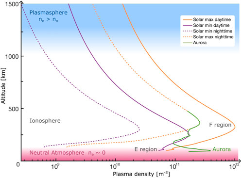
Figure 1. An illustration of the high-latitude plasma density as a function of altitude and time (day/night and solar minimum/maximum), estimated by the International Reference Ionosphere (Bilitza, Dieter et al., 2014) above the EISCAT facilities in Ramfjordmoen, Norway. Ionization by auroral precipitation greatly enhances the plasma density in the E-region, making the Arctic ionosphere more complex than the ionosphere at mid and equatorial latitudes. The green line illustrates the enhanced plasma density during auroral conditions, calculated by the mean plasma density under auroral conditions observed by EISCAT on 12th December 2006, from 16.00 to 23.00 UT.
Nearly a century ago, Breit and Tuve (1925, 1926) provided the first experimental evidence of the ionosphere by observing that pulsed high-frequency radio waves are reflected by a conducting and variable layer in the upper atmosphere. Their observations were made by the first version of an ionosonde, a radar system that is still in active use today with more than 100 ionosondes being deployed worldwide (Xiao et al., 2020). An ionosonde consists of an antenna and a receiver that transmit and receive pulsed radio waves that are swept through the typical ionospheric plasma frequency range (0.5 MHz–20 MHz). The distance to the reflection point is calculated from the time delay of the signal from the transmitter to the receiver and is referred to as the virtual distance in this article. Radio waves transmitted vertically are reflected when the transmitted frequency (fT) is equal to the local plasma frequency (fp), i.e., (fT = fp), while waves transmitted at an angle are reflected at lower altitudes due to refraction in the ionosphere. The plasma frequency in the ionosphere is related to the local plasma density by:
this expression can therefore be used to estimate the altitude profile of the plasma density (ne(z)) up to the altitude of the maximum plasma frequency in the E− and F-region. Here, (e) is the elementary charge, (me) is the electron mass and (ϵ0) is the permittivity of free space. Additionally, ionosondes transmit both left-hand and right-hand circular polarized waves, commonly referred to as the Ordinary mode (O-mode) and Extraordinary mode (X-mode) waves, respectively. Note that these mode definitions are traditionally opposite in the fields of physics and engineering (Rexer, 2021). Radio waves transmitted in these two modes are reflected at different altitudes in the ionosphere. In this work, we focus on the O-mode reflection whenever the O- and X-mode traces can be discerned in the F-region.
The ionogram is the basic data product acquired by the ionosonde. The ionogram is a 2-D visualization of the received echo as a function of transmitted frequency and virtual distance (time-of-flight). Each ionosonde typically produces an ionogram every 1–15 min, resulting in several thousand ionograms every month. This data can be used to support ionospheric observations from radars (Patra et al., 2009) and rockets (Savio Odriozola et al., 2017; Neelakshi et al., 2022) and to track both long-term ionospheric trends (Xu et al., 2004) and more transient ionospheric features, such as traveling ionospheric disturbances (Pederick et al., 2017).
Several tools have been developed to extract important features from ionograms automatically, e.g., Autoscala (Scotto and Pezzopane, 2002; Pezzopane and Scotto, 2007), Univap Digital Ionosonde Data Analysis (UDIDA) (Pillat et al., 2013) and other methods, see for example,: Ding et al. (2007); Jiang et al. (2013, 2015); Chen et al. (2018). In addition, automatic methods specialized for processing oblique ionograms have been developed, see for example,: (Ippolito et al., 2015; Song et al., 2016; Jiang et al., 2022). Automatic Real-Time Ionogram Scaling with True-heights (ARTIST), version 5, is currently the most widely used routine (Reinisch and Xueqin, 1983; Galkin and Reinisch, 2008). However, ARTIST-5 achieves sub-optimal performance compared to human scaling, in particular for low signal-to-noise ratio data (Xiao et al., 2020). Themens et al. (2022) compared the ARTIST-5 performance to ∼35 000 manually analyzed ionograms acquired by the Global Ionospheric Radio Observatory (GIRO). They concluded that ARTIST accurately extracts the F2-layer O-mode frequency and the F-region height for ionograms with high confidence scores (
More recently, supervised deep learning methods, in particular deep convolutional neural networks (CNNs), have been implemented for automatic ionogram analysis with promising results. Deep convolutional neural networks are versatile algorithms designed for processing grid-like data, such as image (Krizhevsky et al., 2012; Clausen and Nickisch, 2018), video (Karpathy et al., 2014; Redmon et al., 2016) or time series (Wang et al., 2017; Kvammen et al., 2023). Deep, in this context, refers to the multi-layered architecture of the convolutional neural networks, often consisting of millions of free parameters that are optimized using manually labeled observations (i.e., ionograms) to solve the task at hand. Mochalov and Mochalova (2019) used ∼40 000 manually scaled ionograms from the Parus-A ionosonde, operated by the Pushkov Institute of Terrestrial Magnetism, near Moscow, Russia, to develop a deep neural network for detecting the ionospheric trace and separating the E, F1, and F2-region traces. Xiao et al. (2020) implemented and evaluated several convolutional neural network architectures to identify the E, F1 and F2-region traces using ∼20 000 ionograms from the DPS4D ionosonde near Wuhan, China. Xiao et al. (2020) concluded that the DIAS model (based on the ResNet-50 architecture) achieved the highest performance, outperforming ARTIST and obtaining scaling accuracies close to human experts. De La Jara and Olivares (2021) used convolutional neural networks to accurately detect the ionospheric echo using ∼51 000 ionograms from the Jicamarca VIPIR ionosonde near Lima, Peru, and further developed methods to isolate the ionospheric trace from noise and interference. Rao et al. (2022) implemented a pre-trained VGG-16 convolutional neural network to classify ionograms acquired by the Canadian Advanced Digital Ionosonde (CADI) system in Hyderabad, India. Rao et al. (2022) used 40 000 ionograms to develop the VGG-16 model, achieving a classification accuracy of 97% and an F1-score of 89%, and further demonstrated that the VGG-16 network provided useful outputs even under highly disturbed geomagnetic periods. Finally, Sherstyukov et al. (2023) tested several convolutional neural network architectures for processing ionograms acquired at high latitudes. A large data set consisting of 86 500 ionograms from the Sodankylä Geophysical Observatory was used. Sherstyukov et al. (2023) concluded that the InceptionV3 architecture achieved the highest performance, achieving 87.3% E-region classification accuracy and 92.8% F-region accuracy, and frequency scaling estimates with ∼0.10 MHz mean absolute error.
Following the previous work, the main purpose of this study was to develop a deep convolutional neural network specialized for processing high-latitude oblique ionograms. The high-latitude ionosphere is different from the low- and mid-latitude ionosphere due to differences in, for example, particle precipitation, solar zenith angles and plasma convection patterns (Ratovsky et al., 2014). Thus, automatic tools developed for processing low and mid-latitude oblique ionograms are sub-optimal for processing high-latitude data. In addition, previous implementations of deep neural networks have focused mainly on automatically detecting and isolating the ionospheric trace, while we use a somewhat different approach, more similar to Sherstyukov et al. (2023). In this work, we seek to automatically classify ionograms into categories (E-region, F-region and no ionospheric trace) and further quantify the characteristic E− and F-region virtual distances and maximum frequencies. This study was further motivated by the expected increased number of high-frequency radar sounders in Fennoscandia, and a great demand for reliable monitoring of the ionosphere in relation to the anticipated EISCAT 3D incoherent scatter radar in Skibotn, Norway (McCrea et al., 2015).
This work focuses on ionograms acquired by the Network of Oblique Ionospheric Receivers Experiment (NOIRE) (Floberg, 2022). NOIRE consists of 4 oblique sounding receivers positioned in Skibotn, Oulu, Kuusamo and Ivalo, illustrated in Figure 2. These receivers are linked to the ionosonde transmitter located in Sodankylä and operated by the Sodankylä Geophysical Observatory (Kozlovsky et al., 2013; Enell et al., 2016). Each receiver station is equipped with an active magnetic loop antenna and a universal Software Radio Peripheral (USRP) platform. NOIRE acquires one ionogram on each minute, resulting in 1440 ionograms each day at all receiver stations. The ionograms have dimension (310 × 310), 310 transmitted frequencies spanning linearly between 0.5 MHz and 16 MHz and 310 range gates spanning linearly between 200 km and 1500 km.
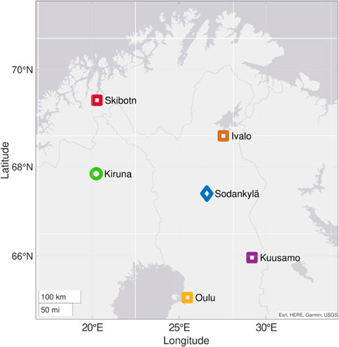
Figure 2. NOIRE consists of 4 oblique sounding receivers positioned in Skibotn, Oulu, Kuusamo and Ivalo. The NOIRE receivers are linked to an ionosonde transmitter located in Sodankylä. This work focuses on ionograms acquired by the Skibotn receiver, with a skip distance of 338.8 km (Floberg, 2022). Additional receiver stations will be installed in Fennoscandia in the upcoming years. Auroral images from the All-sky camera in Kiruna, operated by the Swedish Institute of Space Physics, are used to infer auroral conditions i n this study.
For the purpose of this study, ionograms acquired in Skibotn between 2022-04-01 and 2023-04-01 are considered. Figure 3 summarizes the solar and geophysical background conditions during this period. The data has a good representation of the seasonal variability, with more than 1000 monthly ionograms, and a broad coverage of the solar elevation angles. However, a wider range of solar and geophysical conditions would be beneficial, e.g., over an entire solar cycle, but is unobtainable since NOIRE has only been in operation (with the current software) since 2022. The framework outlined in this article can however be used to extend the considered dataset in future work. The proposed methodology can further be used to include ionograms from other receiver stations and even other ionosondes with additional training.
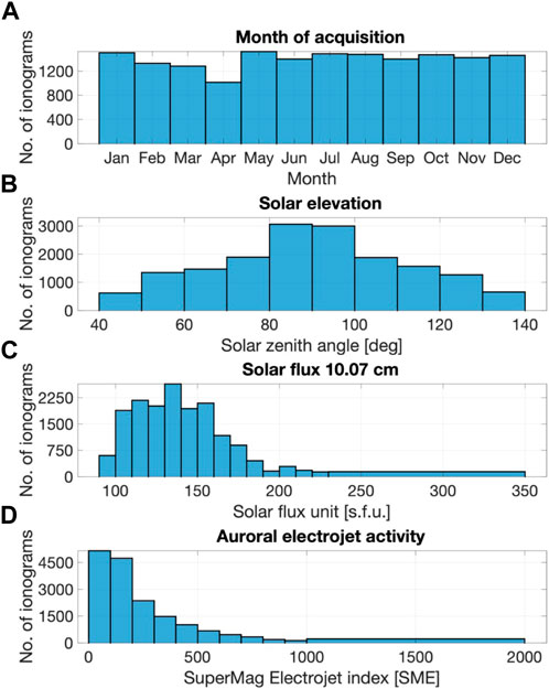
Figure 3. Histograms of solar and geophysical indices during periods of ionogram acquisition. (A) summarizes the number of ionograms for each Month. (B) the solar elevation is highly correlated to the F-region frequency, the histogram indicates a balanced data set around a 90-degree solar zenith angle. (C) The solar radiation flux in the 10.7 cm wavelength is an indication of solar activity King and Papitashvili (2005), the histogram indicates good coverage between ∼90-160 s. f.u. Note that the bins are 10 s. f.u. from 90 to 230 s. f.u. and a single bin from 230 to 350 s. f.u. (D) The SuperMAG electrojet index (SME) estimates the ionospheric current in the auroral oval by evaluating the magnetic H-component across more than 100 magnetometer stations near the auroral oval Bergin et al. (2020); Newell and Gjerloev (2011). The histogram indicates that ionograms were acquired over a range of auroral activities, with good coverage over SME values ranging from 100 to ∼500. A high SME value indicates enhanced auroral activity and is correlated to the E-region maximum frequency. The bins are spaced from 0 to 1000 with a bin size of 100 SME, and a single bin from 1000 to 2000 SME.
The ionogram data is preprocessed in order to enhance the ionospheric trace and standardize the input to the convolutional neural network. Standardized data further makes manual scaling more consistent and eases parameter optimization during training. A 3-step preprocessing procedure was used on each ionogram in the considered data set (Figure 4 illustrates the step-by-step procedure on a sample ionogram).
1. Noise normalization: Each column (i.e., frequency channel) of the ionogram is independently normalized by division of the median absolute deviation. This is done to clean the ionograms from radio and high-frequency communication interference.
2. Min-max cap: The received ionograms typically contain a wide range of values. The ionospheric echo is of interest, not the signal strength, which can vary up to 6 orders of magnitude. The pixel values are therefore capped between 0 and 20, meaning that intensities below 0 are set to 0 and intensities above 20 are set to 20. The min-max capping ensures a more robust representation under variable ionospheric conditions.
3. Pixel normalization: The ionogram pixel values are scaled to [0,255] for efficient 8-bit image storage. The images are however normalized to a pixel range [0,1] before network training and testing.
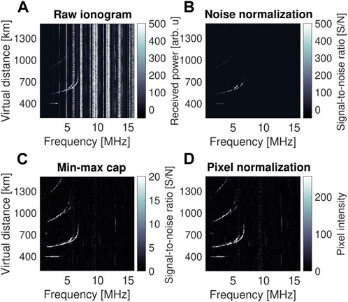
Figure 4. The 3-step preprocessing procedure. (A) displays the raw ionogram, acquired on 15 November 2022, at 13:44 UT in Skibotn. The ionogram processed by step 1: noise normalization, is shown in (B). (C) displays the ionogram after step 2: min-max cap. (D) shows the ionogram after being processed by step 3: pixel normalization.
Supervised machine learning techniques require manually labeled data to both train and test the classifiers (Goodfellow et al., 2016, p 101–102). Attention is therefore needed in order to construct a high-quality labeled data set that can be used to develop reliable classifiers without significant contamination of biases, corrupted data files and mislabeled ionograms (McKay and Kvammen, 2020). For this work, a two-step routine was employed. The initial step involves the classification of ionograms based on the features of interest, namely, the presence or absence of a clearly discernible E-region and/or F-region trace. These two binary classifications yield four categories: E-region, F-region, E and F-region and no trace. The second step is manually identifying the E-region and/or F-region virtual distance and maximum frequencies (if traces are present). Figure 5 presents examples of ionograms with E-region, F-region, E and F-region and no trace, along with the manual scaling for the positive classes. Table 1 presents the number of ionograms in each class.
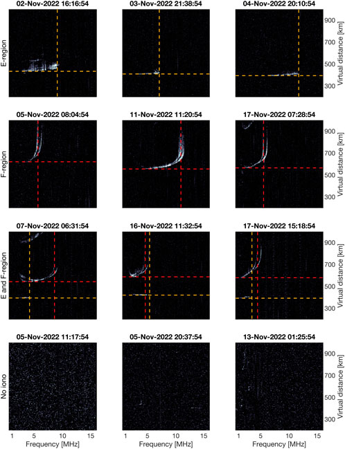
Figure 5. Each ionogram is classified based on the presence or absence of a clearly visible E-region and/or F-region trace. Examples of ionograms with a clearly visible E-region trace are presented in the top row along with the manually scaled E-region virtual distance and maximum frequency (indicated by the yellow lines). The third E-region example displays an E-region trace under auroral conditions. The second row displays typical F-region profiles with the manual scaling in red. Note that two F-region traces can often be observed, the echo from the transmitted O-mode frequency and the X-mode frequency with slightly higher frequency values, we focus on extracting the maximum usable O-mode frequency. Ionograms with both E-region and F-region traces are presented in the third row. In the case of a clearly visible F1-layer, as in example 1, the F1 virtual distance is scaled. The bottom row presents examples of ionograms without a clearly visible ionospheric trace.
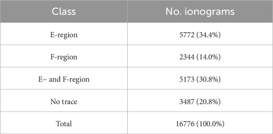
Table 1. The manually labeled and scaled ionograms. This data set is used to train, validate and test the convolutional neural networks. The random draw results in a fairly balanced number of observations for each class with a 65.2% probability for an E-region trace and a 44.8% probability for a clear F-region trace.
In practice, each ionogram was drawn randomly from the considered data set (without replacement) and displayed. A Graphical User Interface (GUI) was then used to implement the two-step routine, making it easy for the human user to assign an ionogram class and the relevant scaling parameters rigorously and efficiently. In total, 16 776 ionograms were manually classified and scaled by 5 different scientists with knowledge of the salient ionogram features.
The manually analyzed data was chronologically sorted and split into training, validation and testing sets using a 10-fold cross-validation approach (Hastie et al., 2009). This method divides the sorted data into 10 subsets (or folds) with approximately equal size (Chollet, 2021; Varoquaux and Colliot, 2023). 8 folds (∼224 h of data) was used for training the convolutional neural networks, one fold (∼28 h) was used for validating the models and the last fold was held out for testing. 10 convolutional neural networks were then developed using different data subsets through circular permutation, illustrated in Figure 6, allowing the mean performance across the 10 networks to be reported with error estimates.
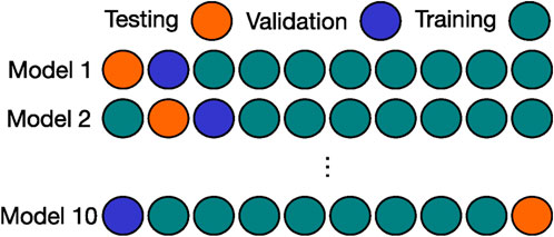
Figure 6. The manually analyzed ionograms in Table 1 were chronologically sorted and split into 10 subsets (folds), each fold is illustrated by a colored circle. 10 convolutional neural networks were then developed using different subsets of the data, 8 folds were used for training the models (illustrated in teak), one fold for validation (blue) and one fold was left out for testing the trained networks (orange). This method ensures that all ionograms are used for training, validation and testing, while being robust to time-correlated observations.
The 10-fold cross-validation approach was implemented to minimize the number of observations in the validation and testing sets with a high correlation (in time) to the ionograms in the training data. Highly correlated ionograms are problematic since near-consecutive observations are likely to be similar, leading to an overestimation of the reported performance (Camporeale, 2019). Note that a random split would cause approximately one-third (on average 36.2% ± 0.9%) of the validation and testing data to be highly time-correlated with the training data. Highly time-correlated observations are defined here as ionograms that are separated by no more than 10 min.
This project aimed at developing a tool that can take an ionogram as input and automatically output the ionogram class and the ionogram scaling parameters for the positive classes. Mathematically, the objective becomes to find a non-linear function (f), parameterized using the trainable weights and biases (w), that maps an input ionogram (x) to the output class or scaling parameters (y), this yields Eq. 2:
In this work, the free parameters (w) are structured in a CNN consisting of 12 convolutional layers and 3 fully connected layers, which implements the non-linear function f (w, x). For an introduction to convolutional neural network designs see e.g., Goodfellow et al. (2016, Chapter 9). The employed CNN, named NOIRE-Net, is illustrated in Figure 7 and the number of free parameters in each layer are summarized in Table 2.
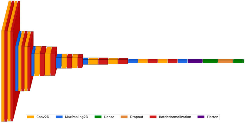
Figure 7. Visualization of the NOIRE-Net architecture, made using the visualkerasprogram (Gavrikov, 2020). The CNN consists of 12 convolutional layers, 6 maximum pooling layers and 3 fully connected layers. This architecture implements f (w, x), the non-linear function that maps the input ionogram (x) to the output class or scaling parameters (y).
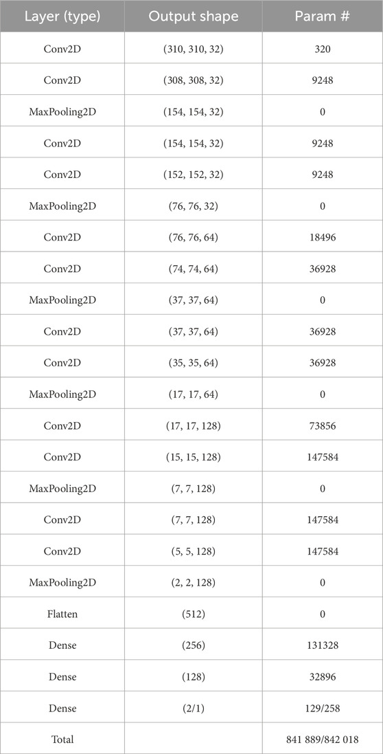
Table 2. The NOIRE-net architecture consists of ∼842 000 free parameters, the exact number depends on the task. The last layer with one output is for classifying the presence of an E-region trace or classifying the presence of an F-region trace. The last layer with two outputs is used for the regression of the E-region virtual distance and maximum frequency or the regression of the F-region virtual distance and maximum O-mode frequency. The input images all have dimensions (310 × 310 × 1), and this is also the expected input format to NOIRE-Net. The size of the information “volume”, as information propagates from the input image through the network, can be tracked by the output shape, where the last dimension represents the number of filters in each layer. Each 2D convolutional layer (Conv2D) and fully connected layer (Dense), except for the last layer, employs the rectified linear unit (ReLU) as the activation function. All 2D convolutional layers use a kernel size of (3,3) to define the filters.
The rectified linear unit (ReLU) was used as the activation function (Nair and Hinton, 2010), i.e., the function that determines the activation of the neurons in hidden layers based on the network weights and the input ionogram. Six maximum pooling layers were introduced to the network in order to downscale the data as information propagates through the network while extracting the most important features (Zhou and Chellappa, 1988). Batch normalization (Ioffe and Szegedy, 2015) was added after each convolutional layer to stabilize the learning process while dropout (Srivastava et al., 2014) was added between two of the fully connected layers to prevent overfitting. This architectural design was influenced by well-known CNN designs such as AlexNet (Krizhevsky et al., 2012) and VGG (Simonyan and Zisserman, 2015). The main difference is that NOIRE-Net was adapted to the specific input image size of the ionograms.
In order to solve the ionogram classification and scaling tasks, four CNNs were trained, these CNNs are jointly referred to as NOIRE-Net.
1. E-classify: This network was trained to classify the ionograms into two predefined labels: E-region or no E-region, indicating the presence or absence of an E-region trace, see Figure 5 for examples.
2. F-classify: The F-classify network was optimized to catalog ionograms into the binary labels: F-region or no F-region.
3. E-scale: This network was trained to solve the regression task of determining the E-region maximum frequency and the E-region virtual distance for cases where an E-region exists.
4. F-scale: The F-scale network was developed to find the F-region maximum usable O-mode frequency and the virtual distance for cases where an F-region is clearly visible.
As commonly used for binary classification tasks with CNNs, a logistic sigmoid activation function
The parameters (w) were optimized using stochastic gradient descent (Adam algorithm) (Kingma and Ba, 2017) and the training data set, consisting of input-output pairs (xi, yi). For the labeling task, we used the binary cross-entropy between the distribution of true (yi) and predicted (f (w, xi)) labels to define the loss function (Theodoridis and Koutroumbas, 2009b, p 172–173), as expressed in Eq. 3:
where
For the regression task of estimating the E− or F-region virtual distance and maximum frequencies, a sum of squared errors between the manually scaled parameters (yi) and the predictions (f (w, xi)) was used as the loss function (Theodoridis and Koutroumbas, 2009a, p 108–109), as expressed in Eq. 4:
The CNNs were implemented using the TensorFlow and Keras frameworks. The training was conducted on a MacBook Pro with a M1 Max 32-core GPU and required about 2 h for each network. A dynamic learning rate between 0.001 and 1 ⋅10–5 over 100 epochs with a batch size of 64 was used to optimize the network parameters. These hyper-parameters were selected after a few experimental runs with different parametrizations. The effect of varying dropout rates, optimization methods and activation functions are unexplored. A systematic tuning of all these hyper-parameters, e.g., using an automatic optimization tool like Optuna Akiba et al. (2019), might further enhance the NOIRE-Net performance, but was not attempted in the interest of time. For more information about the training and testing of NOIRE-Net, please visit the relevant Notebooks at https://github.com/AndreasKvammen/NOIRE-Net/.
The classification and scaling performances of NOIRE-Net are evaluated using the testing data. We report the average performance from 10 independent training runs with random initialization of the NOIRE-Net weights and biases (w). For each training run, the manually labeled and scaled ionograms are split into training, validation and testing data sets with a (0.8, 0.1, 0.1) partitioning using the 10-fold cross-validation method described in Section 2.3. This approach, using the ensemble performance from 10 runs, provides a more robust performance and further allows for error estimates between the trained CNNs.
Table 3 presents the performance scores of NOIRE-Net for the classification task. The classifier is compared to a simple baseline probability model. The probability model randomly predicts the class of the ionogram based on the probability of a positive class (65.2% for the E-region and 44.8% for the F-region), calculated using the manually labeled data in Table 1. NOIRE-Net outperforms the probability model across all metrics. NOIRE-Net achieves a reliable E-region classification performance with very high (≥0.9) scores over all metrics, see the Appendix for the definitions of the evaluation metrics. For the F-region, NOIRE-Net archives a good performance (≥0.85) for the precision and accuracy metrics but has a lower score for the recall (0.81 ± 0.15) and F1-score (0.84 ± 0.01). This indicates that some observations that were manually labeled as F-region are misclassified (no F-region) by NOIRE-Net.
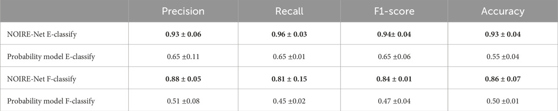
Table 3. Summary of the classification performance. NOIRE-Net achieves high (≥0.90) performance scores over all metrics for the E-region classification and an acceptable (≥0.85) performance for the F-region precision and accuracy, but has a lower score for the recall and F1 score(0.81 ±0.15 and 0.84 ±0.01).
Figure 8 presents the NOIRE-Net performance as confusion matrices. Overall, NOIRE-Net achieves a reliable E-region classification performance and a good performance for the F-region classification, although with a significant (19% ± 15%) proportion of false negative F-region observations (as expected from the lower recall score).
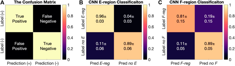
Figure 8. (A) The confusion matrix is populated by the true (correctly classified) and false (erroneously classified) observations, as compared to the manual labels. Positive (+) ionograms indicate the presence of an E/F trace while negative (−) ionograms indicate the absence of an E/F trace. (B) The CNN E-region classification performance. 96% ±3% of the observations manually labeled to contain an E-region trace are correctly predicted by the CNN, while 89% ±6% of the ionograms without E-region traces are correctly classified by the CNN. (C) The performance of F-region classification. The CNN correctly classifies 81% ±15% of the ionograms with a clearly visible F-region trace while 89% ±5% of ionograms without F-region traces are correctly predicted.
The scaling performance of NOIRE-Net is evaluated by the median absolute deviation (MAD) and the root mean square error (RMSE). Table 4 summarizes the performance for each output parameter across 10 training runs. The NOIRE-Net scaling performance is compared to a mean reference model. The mean model always predicts the mean value of the scaling parameters, 6.21 MHz for the E-region maximum frequency and 6.07 MHz for the F-region maximum O-mode frequency, and 404 km and 611 km for the virtual distances, respectively.
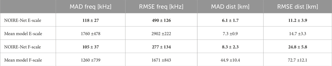
Table 4. Summary of the scaling performance. NOIRE-Net provides scaling parameters with MAD values within 3 pixels for the E and F-region scaling.
Overall, NOIRE-Net outperforms the mean model and provides scientifically useful outputs with MAD values of 118 kHz ±27 kHz for the E-region maximum frequency and 105 kHz ±37 kHz for the F-region maximum O-mode frequency. Predictions of the virtual distance for the E− and F-region yield MAD values of 6.1 km ± 1.7 km and 8.3 km ± 2.3 km. Note that the ionograms have dimensions (310 × 310), with 50 kHz frequency resolution and a ∼4.2 km virtual distance resolution for each pixel. Thus, NOIRE-Net provides predictions with MAD values within 3 pixels of manually scaled E and F-region traces. The RMSE values are sensitive to outliers and NOIRE-Net archives RMSE values within 10 pixels. The E-region frequency is the most uncertain parameter, indicating a significant number of outliers, possibly due to specular meteor trail echoes (Ellyett and Goldsbrough, 1976) and a large variability from quiet to auroral conditions.
In this section, the NOIRE-Net performance is studied by analyzing the stability across the parameter space and by evaluating the consistency (in time) during both quiet and active auroral conditions. These analyses are performed using additional testing data sets, auxiliary to the manually labeled and scaled data set presented in Table 1.
The stability of NOIRE-Net across the parameter space is studied by analyzing the performance on an additional testing data set consisting of 652 ionograms. In this data set, each ionogram was labeled and scaled by 1-5 human experts, with a mean value of 3.92 human experts per ionogram. A summary of this data set is presented in Table 5. The NOIRE-Net scaling predictions are compared to the multi-human analysis in Figure 9. Note that ionograms in the multi-human data set (Table 5) with a high time correlation to the observations in the NOIRE-Net data set (Table 1) were excluded. In total 46.2% of the multi-human data was rejected due to high time correlation, excluding ionograms acquired within 10 min of an observation in Table 1. Still, the remaining data presented in Figure 9 contain the 48.5% semi-correlated ionograms (observations sampled within 10-20 min) and might present an overestimated performance compared to data outside the time domain of the NOIRE-Net data set.
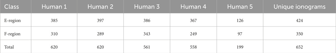
Table 5. The manually labeled and scaled ionograms used for testing the stability of NOIRE-Net across the parameter space. Each ionogram was labeled and scaled by 1-5 humans. Note that a single ionogram can contain both an E-region trace and an F-region trace. In total, 652 unique ionograms were analyzed.
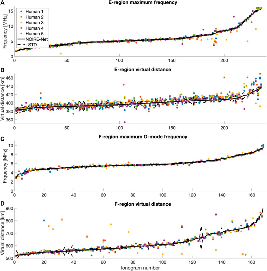
Figure 9. A comparison of the multi-human and NOIRE-Net scaling predictions across the output parameter space. The ionogram number is sorted by increasing NOIRE-Net output values. (A) presents the E-region maximum frequency comparison. A few outliers can be seen, but there is no clear skew between the human and NOIRE-Net scaling. Note that the ±standard deviation values around the median NOIRE-Net predictions across the 10 CNNs are included, but are generally too small to be seen within the human vs. human spread. (B) displays the E-region virtual distance comparison. The E-region virtual distance has a small range in output values and the NOIRE-Net scaling is in line with human interpretation. (C) The F-region maximum frequency has a large dynamic range, still, the agreement between NOIRE-Net and the human scaling is consistently good. (D) Overall, the NOIRE-Net predictions of the F-region virtual distance are in-line with human interpretation, however, a few outliers can be seen spread across the parameter space. A possible reason for these outliers is ambiguity in F1-layer or F2-layer scaling, which is not treated separately in this project (the lowermost F-region trace is defined as the F-region height).
In summary, Figure 9 indicates that NOIRE-Net provides scaling parameters that are generally in-line with the human interpretation. A few outliers can be seen, especially for the E-region maximum frequency and the F-region virtual distance, as already implied by the large RMSE values in Table 4. It should be noted that ionograms with low signal-to-noise ratios are often ambiguous, and the “correct” class and scaling parameters differ from person to person. Still, there is no clear skew between the NOIRE-Net predictions and the human consensus, suggesting that NOIRE-Net provides scientifically useful scaling results across the parameter space.
Consecutive ionograms acquired over a 24-h period (24 October 2022) were manually analyzed to study the self-consistency of NOIRE-Net (in time). Furthermore, this data set was used to compare NOIRE-Net and human analysis during both quiet and active auroral conditions. A summary of this data set is presented in Table 6. Ionograms from 24 October 2022 were selected for this analysis since auroral emissions were clearly visible in the Kiruna all-sky camera for a longer period (21:00-00:00) without cloud contamination or significant light pollution from the moon or other sources. Figure 10 presents the comparison of the NOIRE-Net and human classification and scaling. A movie of the NOIRE-Net performance on this data is added to the Supplementary Material.
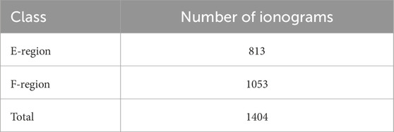
Table 6. The manually labeled and scaled ionograms used for analyzing the NOIRE-Net stability in time. Note that the E-region and F-region labels are not mutually exclusive. In total, 1404 ionograms were analyzed.

Figure 10. Manually analyzed ionograms are compared to the NOIRE-Net predictions during a 24-h period (October 24, 2022) in subplots (A–D). The error bars mark the standard deviation around the median, calculated using outputs from 10 independently trained CNNs. Classification disagreements can be seen as periods where there are either NOIRE-Net predictions or human scaling. Disagreement is seen in the E-region for ionograms with high maximum frequencies that only last for one ionogram frame (likely due to specular meteor trail echoes) and some disagreement can be seen in the frequency scaling during auroral conditions (characterized by high maximum frequencies that last for longer periods). Some disagreements are also seen in the F-region around 04:30 UT and around 21:00 UT, these disagreements are due to ambiguous and/or weak F-region echoes, as displayed by the example ionograms from 03:00 UT and 21:00 UT in subplots (E) and (G). The dotted red lines in subplots (E–G) represent the ± standard deviation values around the median predicted values across the 10 CNNs. In general, NOIRE-Net provides stable outputs (in time) that are mostly in-line with human interpretation. Note, however, that for ionogram (E), the human erroneously scaled the F-region X-mode trace while NOIRE-Net correctly scaled the O-mode maximum frequency. In addition, there is no NOIRE-Net F-region scaling in subplot (G) since NOIRE-Net provided a negative F-region label for this ionogram while the human classified the ionogram as containing an F-region, the ionogram has a low signal-to-noise ratio and the “true” label is ambiguous.
Figure 10 demonstrates that NOIRE-Net scaling generally follows human interpretation under various conditions and further provides self-consistent outputs (in time) with few outliers. Figure 10 further suggests that inconsistency predominantly occurs for ambiguous ionograms, often with low signal-to-noise ratios, ionograms that are difficult to interpret for human experts as well. In addition, NOIRE-Net provides some disagreement with human interpretation under auroral conditions, as seen in the E-region maximum frequency scaling in Figure 10A.
Figure 11 investigates the E-region maximum frequency prediction in detail for a variable period 21:00-00:00 with auroral precipitation. The observed green-line intensity enhancement (I5577) is approximately proportional to the production of secondary electrons (qe) from precipitating particles (Rees and Luckey, 1974). Further, at E-region heights during steady-state, the electron density is proportional to
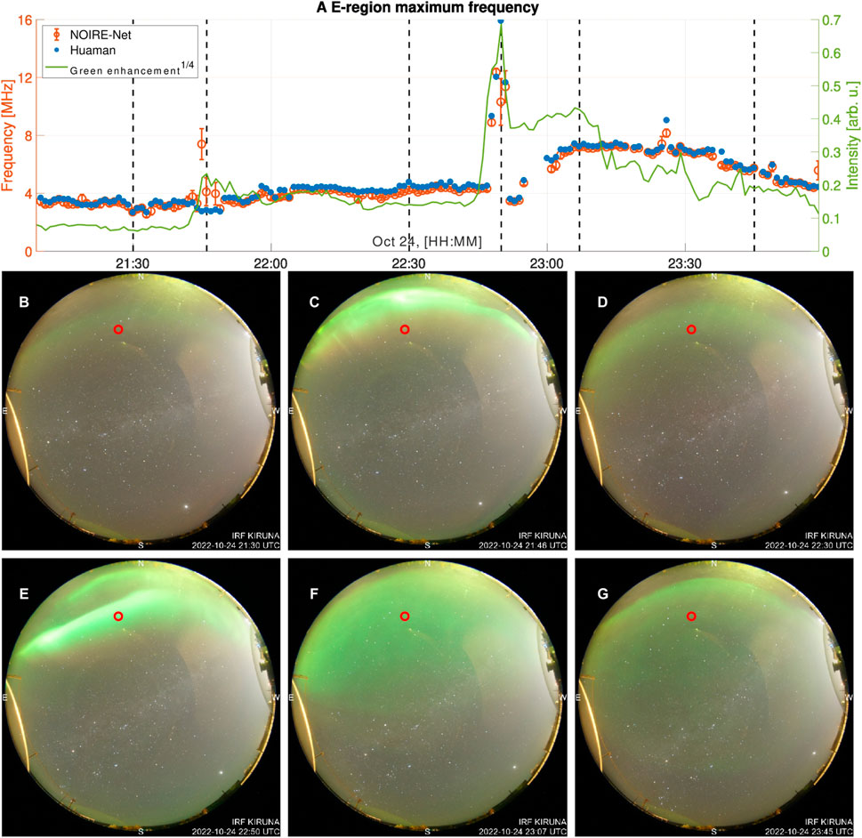
Figure 11. The top row (A) compares the E-region maximum frequencies predicted by NOIRE-Net to the manual scaling during variable auroral activity on October 24. The black vertical lines indicate the time-stamps of the images, acquired by the Kiruna all-sky camera. The red circle marked in each image indicates the refraction point of the radio waves from the transmitter in Sodankylä to the receiver station in Skibotn. The refraction point is estimated by calculating the location of the midpoint on a great circle between the transmitter and the receiver, projected to an altitude of 110 km in the camera field-of-view using star calibration. The fourth root of the green-light mean pixel intensity enhancement around this point is plotted in green. Strong auroral emissions appear north of the refraction point around 21:45 UTC, as displayed in (C), with less active conditions both before, shown in (B) at 21:30 UTC, and after, as illustrated in (D) at 22:30 UTC. The auroral display is enhanced around the same time as the E-region maximum frequency is enhanced, as predicted by NOIRE-Net although not for the manual scaling. Later, a stronger auroral enhancement suddenly appears around 22:50 UTC within the refraction point, as shown in (E). A sharp E-region maximum frequency increase can be seen at the same time in both the NOIRE-Net prediction and the human scaling. After this point, both the E-region maximum frequency and the auroral intensity decrease as shown in (F)at 23:07 UTC and in (G)at 23:45 UTC.
In this study, deep convolutional neural networks have been trained and tested for automatic classification and scaling of high-latitude oblique ionograms. Overall, the trained networks (jointly named NOIRE-Net) obtained reliable outputs in-line with human interpretation. NOIRE-Net achieved an average classification accuracy of 93% ± 4% for the E-region and 86% ± 7% for the F-region. Furthermore, NOIRE-Net obtained scientifically useful scaling parameters with median absolute deviation values of 118 kHz ±27 kHz for the E-region maximum frequency and 105 kHz ±37 kHz for the F-region maximum O-mode frequency. Predictions of the virtual distance for the E− and F-region yielded median distance deviation values of 6.1 km ± 1.7 km and 8.3 km ± 2.3 km, respectively. In general, NOIRE-Net therefore achieves scaling performances with median absolute deviation values well within the 95% confidence error bounds of ARTIST-5 (Stankov et al., 2023): E-region O-mode frequency [-0.3 MHz, +0.8 MHz], F2-layer O-mode frequency [-0.35 MHZ, +0.25 MHZ], E-region height [-6 km, +6 km] and F2-layer height [-115 km, +45 km].
The stability of NOIRE-Net over several testing data sets and under auroral conditions has been studied. Overall, NOIRE-Net provides stable classification and scaling performances. Our analysis indicates that disagreement with human interpretation primarily arises for ambiguous ionograms, often with low signal-to-noise ratios or acquired under challenging auroral conditions, i.e., under conditions that are difficult to interpret for human experts as well. An enhanced E-region scaling performance may however be achieved for periods with auroral precipitation by adding auroral conditions as an independent class in the classification network and further train a network specialized for scaling ionograms with clearly discernible auroral features. This additional routine, where auroral ionograms are explicitly cataloged, may provide a useful data product for auroral researchers using ionogram data or data from co-located instruments. Further improvements to NOIRE-Net might be achieved by enriching the training data set, e.g., by adding ionograms from other years (with different solar activity levels), and by systematically tuning the NOIRE-Net hyper-parameters.
Our study concludes that deep convolutional neural networks are suitable for classification and scaling of high-latitude ionograms. The framework outlined in this article may serve as a foundation for implementing ionograms from other NOIRE receiver stations with additional training. Automatic classification and scaling of ionograms acquired by the Network of Oblique Ionospheric Receivers Experiments (NOIRE) will be a great asset for studies of the ionosphere over Fennoscandia in general and in particular for ionospheric monitoring in relation to the anticipated EISCAT 3D incoherent scatter radar in Skibotn, Norway (McCrea et al., 2015).
Publicly available datasets were analyzed in this study. This data can be found here: Ionograms acquired by the Network of Oblique Ionospheric Receivers Experiment (NOIRE) are available at http://kaira.uit.no/juha/noire/. The trained NOIRE-Net models and the replication code for this work can be accessed at https://github.com/AndreasKvammen/NOIRE-Net/ and are freely available under the MIT software license.
AK: Formal Analysis, Investigation, Project administration, Software, Supervision, Validation, Visualization, Writing–original draft, Writing–review and editing, data curation. JV: Conceptualization, Data curation, Methodology, Project administration, Resources, Software, Supervision, Validation, Writing–review and editing. DH: Data curation, Resources, Writing–review and editing, Methodology. TR: Visualization, Writing–review and editing, data curation. AS: Writing–review and editing, data curation. BG: Software, Writing–review and editing. JF: Data curation, Methodology, Writing–review and editing.
The author(s) declare that financial support was received for the research, authorship, and/or publication of this article. AK, TR, and AS acknowledge support from the Research Council of Norway grant 326039. JV acknowledges support from the Tromsø Research Foundation. DH and AS were funded during this study through a UiT The Arctic University of Norway contribution to the EISCAT 3D project, funded by the Research Council of Norway through research infrastructure grant 245683.
The authors would like to thank Urban Brändström and the Swedish Institute of Space Physics for providing the auroral image data. We gratefully acknowledge the SuperMAG collaborators (https://supermag.jhuapl.edu/info/?page=acknowledgement). The 10.7 cm solar flux data was obtained from the GSFC/SPDF OMNIWeb interface at https://omniweb.gsfc.nasa.gov. We would also like to thank the Sodankylä Geophysical Observatory for operating the ionosonde transmitter. Thanks to Filippo Maria Bianchi for valuable recommendations on neural network training and testing. Finally, the authors would like to thank the reviewers for their excellent suggestions and useful comments.
The authors declare that the research was conducted in the absence of any commercial or financial relationships that could be construed as a potential conflict of interest.
All claims expressed in this article are solely those of the authors and do not necessarily represent those of their affiliated organizations, or those of the publisher, the editors and the reviewers. Any product that may be evaluated in this article, or claim that may be made by its manufacturer, is not guaranteed or endorsed by the publisher.
The Supplementary Material for this article can be found online at: https://www.frontiersin.org/articles/10.3389/fspas.2024.1289840/full#supplementary-material
Akiba, T., Sano, S., Yanase, T., Ohta, T., and Koyama, M. (2019). “Optuna: a next-generation hyperparameter optimization framework,” in Proceedings of the 25th ACM SIGKDD International Conference on Knowledge Discovery and Data Mining (New York, NY, USA: Association for Computing Machinery), KDD ’19, Anchorage, AK, USA, August 4 - 8, 2019, 2623–2631.
Bergin, A., Chapman, S. C., and Gjerloev, J. W. (2020). AE, DST, and their SuperMAG counterparts: the effect of improved spatial resolution in geomagnetic indices. J. Geophys. Res. Space Phys. 125, e2020JA027828. doi:10.1029/2020JA027828
Bilitza, D., Altadill, D., Zhang, Y., Mertens, C., Truhlik, V., Richards, P., et al. (2014). The international reference ionosphere 2012 - a model of international collaboration. J. Space Weather Space Clim. 4, A07. doi:10.1051/swsc/2014004
Breit, G., and Tuve, M. A. (1925). A radio method of estimating the height of the conducting layer. Nature 116, 357. doi:10.1038/116357a0
Breit, G., and Tuve, M. A. (1926). A test of the existence of the conducting layer. Phys. Rev. 28, 554–575. doi:10.1103/PhysRev.28.554
Brekke, A. (2012). Physics of the upper polar atmosphere. Cham: Springer Science and Business Media.
Camporeale, E. (2019). The challenge of machine learning in space weather: nowcasting and forecasting. Space weather. 17, 1166–1207. doi:10.1029/2018SW002061
Chen, Z., Gong, Z., Zhang, F., and Fang, G. (2018). A new ionogram automatic scaling method. Radio Sci. 53, 1149–1164. doi:10.1029/2018RS006574
Clausen, L. B. N., and Nickisch, H. (2018). Automatic classification of auroral images from the oslo auroral themis (oath) data set using machine learning. J. Geophys. Res. Space Phys. 123, 5640–5647. doi:10.1029/2018JA025274
De La Jara, C., and Olivares, C. (2021). Ionospheric echo detection in digital ionograms using convolutional neural networks. Radio Sci. 56, 1–15. doi:10.1029/2020RS007258
Ding, Z.-H., Ning, B.-Q., and Wan, W.-X. (2007). Real-time automatic scaling and analysis of ionospheric ionogram parameters. Chin. J. Geophys. 50, 837–847. doi:10.1002/cjg2.1101
Ellyett, C. D., and Goldsbrough, P. F. (1976). Relationship of meteors to sporadic e, 1. a sorting of facts. J. Geophys. Res. (1896-1977) 81, 6131–6134. doi:10.1029/JA081i034p06131
Enell, C.-F., Kozlovsky, A., Turunen, T., Ulich, T., Välitalo, S., Scotto, C., et al. (2016). Comparison between manual scaling and autoscala automatic scaling applied to sodankylä geophysical observatory ionograms. Geoscientific Instrum. Methods Data Syst. 5, 53–64. doi:10.5194/gi-5-53-2016
Floberg, J. (2022). “Design and implementation of an oblique ionosonde receiver,” in For studies of spatial and temporal ionospheric structures (Tromsø, Norway: UiT Norges arktiske universitet). Master’s thesis.
Galkin, I. A., and Reinisch, B. W. (2008). The new artist 5 for all digisondes. Ionosonde Netw. Advis. Group Bull. 69, 1–8.
Gavrikov, P. (2020). visualkeras. Available at: https://github.com/paulgavrikov/visualkeras.
Goodfellow, I., Bengio, Y., and Courville, A. (2016). Deep learning. Massachusetts, United States: MIT Press. Available at: http://www.deeplearningbook.org.
Hastie, T., Tibshirani, R., Friedman, J. H., and Friedman, J. H. (2009). The elements of statistical learning: data mining, inference, and prediction, vol. 2. Cham: Springer. doi:10.1007/978-0-387-21606-5
Hunsucker, R. D., and Hargreaves, J. K. (2007). The high-latitude ionosphere and its effects on radio propagation. Cambridge University Press.
Ioffe, S., and Szegedy, C. (2015). “Batch normalization: accelerating deep network training by reducing internal covariate shift,” in Proceedings of the 32nd International Conference on Machine Learning, (Lille, France: PMLR), vol. 37 of Proceedings of Machine Learning Research, Lille, France, 6-11 July 2015, 448–456.
Ippolito, A., Scotto, C., Francis, M., Settimi, A., and Cesaroni, C. (2015). Automatic interpretation of oblique ionograms. Adv. Space Res. 55, 1624–1629. doi:10.1016/j.asr.2014.12.025
Jiang, C., Yang, G., Lan, T., Zhu, P., Song, H., Zhou, C., et al. (2015). Improvement of automatic scaling of vertical incidence ionograms by simulated annealing. J. Atmos. Solar-Terrestrial Phys. 133, 178–184. doi:10.1016/j.jastp.2015.09.002
Jiang, C., Yang, G., Zhao, Z., Zhang, Y., Zhu, P., and Sun, H. (2013). An automatic scaling technique for obtaining f2 parameters and f1 critical frequency from vertical incidence ionograms. Radio Sci. 48, 739–751. doi:10.1002/2013RS005223
Jiang, C., Zhao, C., Zhang, X., Liu, T., Chen, Z., Yang, G., et al. (2022). A method for automatic inversion of oblique ionograms. Remote Sens. 14, 1671. doi:10.3390/rs14071671
Karpathy, A., Toderici, G., Shetty, S., Leung, T., Sukthankar, R., and Fei-Fei, L. (2014). “Large-scale video classification with convolutional neural networks,” in 2014 IEEE Conference on Computer Vision and Pattern Recognition, Columbus, OH, USA, June 23 2014 to June 28 2014, 1725–1732.
King, J. H., and Papitashvili, N. E. (2005). Solar wind spatial scales in and comparisons of hourly wind and ace plasma and magnetic field data. J. Geophys. Res. Space Phys. 110. doi:10.1029/2004JA010649
Kingma, D. P., and Ba, J. (2017). Adam: a method for stochastic optimization. Available at: https://arxiv.org/abs/1412.6980.
Kozlovsky, A., Turunen, T., and Ulich, T. (2013). Rapid-run ionosonde observations of traveling ionospheric disturbances in the auroral ionosphere. J. Geophys. Res. Space Phys. 118, 5265–5276. doi:10.1002/jgra.50474
Krizhevsky, A., Sutskever, I., and Hinton, G. E. (2012). Imagenet classification with deep convolutional neural networks. Adv. neural Inf. Process. Syst. 25.
Kvammen, A., Wickstrøm, K., Kociscak, S., Vaverka, J., Nouzak, L., Zaslavsky, A., et al. (2023). Machine learning detection of dust impact signals observed by the solar orbiter. Ann. Geophys. 41, 69–86. doi:10.5194/angeo-41-69-2023
McCrea, I., Aikio, A., Alfonsi, L., Belova, E., Buchert, S., Clilverd, M., et al. (2015). The science case for the eiscat_3d radar. Prog. Earth Planet. Sci. 2, 21. doi:10.1186/s40645-015-0051-8
McKay, D., and Kvammen, A. (2020). Auroral classification ergonomics and the implications for machine learning. Geoscientific Instrum. Methods Data Syst. 9, 267–273. doi:10.5194/gi-9-267-2020
Mochalov, V., and Mochalova, A. (2019). Application of deep learning to recognize ionograms. 2019 Russ. Open Conf. Radio Wave Propag. (RWP) 1, 477–479. doi:10.1109/RWP.2019.8810326
Nair, V., and Hinton, G. E. (2010). “Rectified linear units improve restricted Boltzmann machines,” in Proceedings of the 27th International Conference on International Conference on Machine Learning (Madison, WI, USA: Omnipress), ICML’10, Madison, Wisconsin, USA, July 24-27, 1998, 807–814.
Neelakshi, J., Rosa, R. R., Savio, S., Stephany, S., de Meneses, F. C., Kherani, E. A., et al. (2022). Multifractal characteristics of the low latitude equatorial ionospheric e–f valley region irregularities. Chaos, Solit. Fractals 156, 111808. doi:10.1016/j.chaos.2022.111808
Newell, P. T., and Gjerloev, J. W. (2011). Evaluation of supermag auroral electrojet indices as indicators of substorms and auroral power. J. Geophys. Res. Space Phys. 116. doi:10.1029/2011JA016779
Patra, A. K., Venkateswara Rao, N., Phanikumar, D. V., Chandra, H., Das, U., Sinha, H. S. S., et al. (2009). A study on the low-latitude daytime e region plasma irregularities using coordinated vhf radar, rocket-borne, and ionosonde observations. J. Geophys. Res. Space Phys. 114. doi:10.1029/2009JA014501
Pederick, L. H., Cervera, M. A., and Harris, T. J. (2017). Interpreting observations of large-scale traveling ionospheric disturbances by ionospheric sounders. J. Geophys. Res. Space Phys. 122, 12,556–12,569. doi:10.1002/2017JA024337
Pezzopane, M., and Scotto, C. (2007). Automatic scaling of critical frequency fof2 and muf(3000)f2: a comparison between autoscala and artist 4.5 on rome data. Radio Sci. 42, 1–17. doi:10.1029/2006RS003581
Pillat, V. G., Guimarães, L. N. F., Fagundes, P. R., and da Silva, J. D. S. (2013). A computational tool for ionosonde cadi’s ionogram analysis. Comput. Geosciences 52, 372–378. doi:10.1016/j.cageo.2012.11.009
Rao, T. V., Sridhar, M., and Ratnam, D. V. (2022). An automatic cadi’s ionogram scaling software tool for large ionograms data analytics. IEEE Access 10, 22161–22168. doi:10.1109/ACCESS.2022.3153470
Ratovsky, K., Shi, J., Oinats, A., and Romanova, E. (2014). Comparative study of high-latitude, mid-latitude and low-latitude ionosphere on basis of local empirical models. Adv. Space Res. 54, 509–516. Recent Advances in Equatorial, Low- and Mid-Latitude Mesosphere, Thermosphere-Ionosphere System Studies. doi:10.1016/j.asr.2014.02.019
Redmon, J., Divvala, S., Girshick, R., and Farhadi, A. (2016). You only look once: unified, real-time object detection.
Rees, M. H., and Luckey, D. (1974). Auroral electron energy derived from ratio of spectroscopic emissions 1. model computations. J. Geophys. Res. (1896-1977) 79, 5181–5186. doi:10.1029/JA079i034p05181
Reinisch, B. W., and Xueqin, H. (1983). Automatic calculation of electron density profiles from digital ionograms: 3. processing of bottomside ionograms. Radio Sci. 18, 477–492. doi:10.1029/RS018i003p00477
Rexer, T. (2021). Radio wave propagation through the ionosphere. UiT Norges arktiske universitet. Ph.D. thesis.
Russell, C. T., Luhmann, J. G., and Strangeway, R. J. (2016). Space physics: an introduction. Cambridge University Press.
Savio Odriozola, S., de Meneses, F. C., Muralikrishna, P., Pimenta, A. A., and Kherani, E. A. (2017). Rocket in situ observation of equatorial plasma irregularities in the region between e and f layers over brazil. Ann. Geophys. 35, 413–422. doi:10.5194/angeo-35-413-2017
Scotto, C., and Pezzopane, M. (2002). A software for automatic scaling of fof2 and muf(3000)f2 from ionograms.
Sherstyukov, R., Kozlovsky, A., Ulich, T., and Moges, S. (2023). “Deep learning for ionogram parameters scaling at polar region ionosphere,” in 2023 XXXVth General Assembly and Scientific Symposium of the International Union of Radio Science (URSI GASS), Sapporo, Hokkaido, Japan, 19 - 26 August 2023, 1–4.
Simonyan, K., and Zisserman, A. (2015) Very deep convolutional networks for large-scale image recognition.
Song, H., Hu, Y., Jiang, C., Zhou, C., Zhao, Z., and Zou, X. (2016). An automatic scaling method for obtaining the trace and parameters from oblique ionogram based on hybrid genetic algorithm. Radio Sci. 51, 1838–1854. doi:10.1002/2016RS005987
Srivastava, N., Hinton, G., Krizhevsky, A., Sutskever, I., and Salakhutdinov, R. (2014). Dropout: a simple way to prevent neural networks from overfitting. J. Mach. Learn. Res. 15, 1929–1958.
Stankov, S. M., Verhulst, T. G. W., and Sapundjiev, D. (2023). Automatic ionospheric weather monitoring with dps-4d ionosonde and artist-5 autoscaler: system performance at a mid-latitude observatory. Radio Sci. 58, 1–20. doi:10.1029/2022RS007628
Themens, D. R., Reid, B., and Elvidge, S. (2022). Artist ionogram autoscaling confidence scores: best practices. URSI Radio Sci. Lett. 4, 22–0001. doi:10.46620/22-0001
Theodoridis, S., and Koutroumbas, K. (2009a). “Chapter 3 - linear classifiers,” in Pattern recognition Editors S. Theodoridis, and K. Koutroumbas 4 (Boston: Academic Press), 91–150. doi:10.1016/B978-1-59749-272-0.50004-9
Theodoridis, S., and Koutroumbas, K. (2009b). “Chapter 4 - nonlinear classifiers,” in Pattern recognition Editors S. Theodoridis, and K. Koutroumbas 4 (Boston: Academic Press), 151–260. doi:10.1016/B978-1-59749-272-0.50004-9
Varoquaux, G., and Colliot, O. (2023). Evaluating machine learning models and their diagnostic value. Mach. Learn. Brain Disord., 601–630. doi:10.1007/978-1-0716-3195-9_20
Wang, Z., Yan, W., and Oates, T. (2017). “Time series classification from scratch with deep neural networks: a strong baseline,” in 2017 International Joint Conference on Neural Networks (IJCNN), Anchorage, AK, USA, May 14-19, 2017, 1578–1585.
Xiao, Z., Wang, J., Li, J., Zhao, B., Hu, L., and Liu, L. (2020). Deep-learning for ionogram automatic scaling. Adv. Space Res. 66, 942–950. doi:10.1016/j.asr.2020.05.009
Xu, Z.-W., Wu, J., Igarashi, K., Kato, H., and Wu, Z.-S. (2004). Long-term ionospheric trends based on ground-based ionosonde observations at kokubunji, Japan. J. Geophys. Res. Space Phys. 109. doi:10.1029/2004JA010572
Zhou and Chellappa (1988). “Computation of optical flow using a neural network,” in IEEE 1988 International Conference on Neural Networks vol.2, San Diego, CA, USA, 24-27 July 1988, 71–78.
The performance metrics are calculated using the True Positive (TP), True Negative (TN), False Positive (FP) and False Negative (FN) values, defined by comparing the predicted classes and the manually labeled classes, illustrated in Figure 8.
The overall accuracy of the classifier is the proportion of observations that were correctly predicted by the classifier. The accuracy is defined as:
Precision is defined as the proportion of observations predicted by the classifier as a positive class, whose manual label is indeed positive. Precision is therefore calculated as:
Recall is the proportion of observations manually labeled as positive, that were correctly predicted as positive by the classifier. Recall is defined as:
The F1 score acts as a weighted average of precision and recall and is calculated as:
Keywords: ionogram, automatic, classification, scaling, convolutional neural networks, deep learning, ionosonde, high-latitude
Citation: Kvammen A, Vierinen J, Huyghebaert D, Rexer T, Spicher A, Gustavsson B and Floberg J (2024) NOIRE-Net–a convolutional neural network for automatic classification and scaling of high-latitude ionograms. Front. Astron. Space Sci. 11:1289840. doi: 10.3389/fspas.2024.1289840
Received: 06 September 2023; Accepted: 29 April 2024;
Published: 03 June 2024.
Edited by:
Georgios Balasis, National Observatory of Athens, GreeceReviewed by:
Guillerme Bernoux, Université de Toulouse, FranceCopyright © 2024 Kvammen, Vierinen, Huyghebaert, Rexer, Spicher, Gustavsson and Floberg. This is an open-access article distributed under the terms of the Creative Commons Attribution License (CC BY). The use, distribution or reproduction in other forums is permitted, provided the original author(s) and the copyright owner(s) are credited and that the original publication in this journal is cited, in accordance with accepted academic practice. No use, distribution or reproduction is permitted which does not comply with these terms.
*Correspondence: Andreas Kvammen, YW5kcmVhcy5rdmFtbWVuQHVpdC5ubw==
Disclaimer: All claims expressed in this article are solely those of the authors and do not necessarily represent those of their affiliated organizations, or those of the publisher, the editors and the reviewers. Any product that may be evaluated in this article or claim that may be made by its manufacturer is not guaranteed or endorsed by the publisher.
Research integrity at Frontiers
Learn more about the work of our research integrity team to safeguard the quality of each article we publish.