
95% of researchers rate our articles as excellent or good
Learn more about the work of our research integrity team to safeguard the quality of each article we publish.
Find out more
ORIGINAL RESEARCH article
Front. Astron. Space Sci. , 15 May 2024
Sec. Space Physics
Volume 11 - 2024 | https://doi.org/10.3389/fspas.2024.1273079
 Tikemani Bag1*
 R. Kataoka1Y. Ogawa1
 H. Fujiwara2
 Z. Li3Vir Singh4
 V. Sivakumar5
 S. Sridharan6
 P. Pirnaris7
 T. Tourgaidis7
We selected three superstorms (disturbance storm time [Dst] index less than −350 nT) of 2003–04 to study the thermospheric energy budget with a particular emphasis on the thermospheric cooling emission by nitric oxide via a wavelength of 5.3 μm. The nitric oxide radiative emission data are obtained from the Sounding of the Atmosphere by Broadband Emission Radiometry (SABER) instrument onboard the Thermosphere Ionosphere Mesosphere Energetics and Dynamics (TIMED) satellite and the thermosphere ionosphere electrodynamic general circulation model (TIEGCM) simulation. Different energy sources for the magnetospheric energy injection and the thermospheric/ionospheric dissipation processes are calculated using empirical formulations, model simulations, and space-borne and ground-based measurements. The Joule heating rates calculated from different sources showed similar variations but significant differences in the magnitude. The nitric oxide cooling power is calculated by zonally and meridionally integrating the cooling flux in the altitude range of 100–250 km. The satellite observed that cooling flux responds faster to the energy input, as compared to the modeled results. The cooling power increases by an order of magnitude during storm time with maximum radiation observed during the recovery phase. Both the satellite-observed and modeled cooling powers show a strong positive correlation with the Joule heating power during the main phase of the storm. It is found that the maximum radiative power does not occur during the strongest storm, and it strongly depends on the duration of the main phase. The model simulation predicts a higher cooling power than that predicted by the observation. During a typical superstorm, on average, a cooling power of 1.87 × 10⁵ GW exiting the thermosphere is estimated by the TIEGCM simulation. On average, it is about 40% higher than the satellite observation.
The solar wind and the plasma embedded in the interplanetary magnetic field (IMF) are the dominating sources of energy for the coupled magnetosphere–ionosphere system. The interaction between the magnetosphere and IMF controls the solar wind energy input into the magnetosphere (Dungey, 1961). The process of interaction can lead to the well-known phenomenon “the geomagnetic storm” that affects the whole magnetosphere–ionosphere–thermosphere (MIT) system enveloping the space environment of near-Earth satellites (Baker et al., 2004; Eastwood et al., 2017). The largest/strongest geomagnetic storms are usually associated with the high-speed solar wind and extreme values of the southward IMF. When the IMF is southward oriented, an enormous amount of solar wind energy is transferred into the magnetosphere. The solar wind–magnetosphere coupling is about two orders higher for the southward IMF Bz than that for the northward IMF Bz (Tsurutani and Gonzalez, 1994). Consequently, little amount of energy is allowed to enter the magnetosphere if the orientation of the IMF Bz is northward.
Extreme geomagnetic storms (disturbance storm time [Dst]
In addition, solar wind energy deposition, particularly during extreme geomagnetic storms, causes large-scale global perturbations in the MIT system including the thermospheric energetics and dynamics through the processes of Joule heating and energetic particle precipitation (Sinnhuber, 2012). Several studies report on the impacts of the extreme geomagnetic storms on the MIT system (Lu et al., 1988; Vichare et al., 2005; Sutton et al., 2005; Krauss et al., 2015, 2018; Bag et al., 2014, 2021, 2023a, b, Bag., 2018; Bharti et al., 2018; Oliveira et al., 2020; and references therein). Horvath and Lovell (2010) observed the large-scale propagation of ionospheric disturbances and their impact on the equatorial ionization anomaly during extreme geomagnetic storms. Liu and Lühr (2005), by analyzing the CHAMP satellite observations, reported about 400%, 500%, and 800% enhancement in the thermospheric density at 400 km during the extreme storms of 29–30 October 2003, 30–31 October 2003, and 20–22 November 2003, respectively. Similarly, huge thermospheric density enhancement has been reported from different satellite observations and model simulations (Sutton et al., 2005; Krauss et al., 2015; 2018; National Science and Technology Council, 2018).
The primary mechanisms for the dissipation of the solar and magnetospheric energy input into the MIT are the ring current dissipation, auroral particle precipitation, and Joule heating. Among these, Joule heating is by far the dominating mechanism of energy dissipation (Kozyra et al., 1998; Lu et al., 1998) and is of greater importance due to its huge global implications in affecting the neutral species. It was believed that only about 10% of energy input is dissipated through Joule heating and particle precipitation when Perreault and Akasofu (1981) derived the epsilon parameter (Knipp et al., 1998; Lu et al., 1998; Turner et al., 2001; Tanskanen et al., 2002). However, this amount is increasing gradually. Turner et al. (2009) suggested that about 71%, 17%, and 12% of the total energy are transferred to Joule heating, particle precipitation, and ring current, respectively, during coronal mass ejection (CME)-driven storms. About 68%, 22%, and 10% of the total energy is transferred to Joule heating, particle precipitation, and ring current, respectively, during corotating interaction region (CIR) storms. On the other hand, Hajra et al. (2014) reported about 50% of Joule heating during CIR events. The energy partitioning strongly depends on the solar origin of geomagnetic storms (Perreault and Akasofu, 1978; Knipp et al., 1998; Lu et al., 1998; Turner et al., 2001, 2009; Guo et al., 2012; Chen et al., 2014; Verkhoglyadova et al., 2016). It is now established that the CIR-driven storms are more geoeffective than the CME storms because of the longer-time energy depositions. Earlier studies show that the time-integrated energy input during CIR storms can be larger than that during a typical CME-driven storm (Kozyra et al., 2006; Turner et al., 2009). However, during short periods, the strongest CME-driven storms are more geoeffective than the CIR-driven storms as far as thermospheric density is concerned (Krauss et al., 2015, 2018). The ionospheric efficiency exponentially decreases with an increase in the solar wind input for solar wind input less than 3,000 GW (Guo et al., 2012). It also strongly depends on the clock angle and is independent of the dynamical pressure (Lu et al., 1998; Vichare et al., 2005; Alex et al., 2006; DeLucas et al., 2007; Turner et al., 2009; Guo et al., 2012, and references therein).
In addition to the ionospheric processes such as downward molecular heat conduction, vertical advection, and adiabatic heating, the radiative emission by nitric oxide via a wavelength of 5.3 μm also significantly redistributes the energy input during geomagnetic storms (Maeda et al., 1989; 1992; Mlynczak et al., 2003; 2005; Verkhoglyadova et al., 2016). The NO radiative emission at 5.3 μm is the dominating thermospheric coolant at the altitude of 100–300 km and well known as a “natural thermostat” (Kockarts, 1980; Mlynczak et al., 2003). The primary source is the inelastic collision of nitric oxide with atomic oxygen density.
Under low-latitude sun-lit conditions, molecular nitric oxide is produced by the inelastic collision between atomic nitrogen (N2D) and molecular oxygen (Barth, 1992; Richards, 2004; Gardner et al., 2005). In addition, during geomagnetic storms and in the high-latitude region, nitric oxide is generated by particle precipitation through a series of chemical reactions. The N2 molecule is dissociated by the auroral electrons of energy 1–10 keV and ions with an energy of 10–20 keV to produce N(2D), whereas the auroral electrons with energy in the range of 0.3–0.9 keV dissociate molecular nitrogen to produce N(4S) (Barth, 1992; Richards, 2004; Gardner et al., 2005). They, again, interact with oxygen molecules to form NO, as given below:
This reaction mechanism is important above 110 km because it is highly sensitive to the thermospheric temperature (Gardner et al., 2005).
Under geomagnetic quiet conditions, the radiative cooling balances the EUV/UV heating and the chemical heating (Lin and Deng, 2019). The NO cooling emission also affects the long-term trend of the thermospheric temperature and density. By using the Global Ionosphere Thermosphere Model simulation, Lin and Deng (2019) reported about −17% decadal change in the total NO cooling power during 1982–2013. The NO cooling emission also strongly depends on the solar activity. Li et al. (2018) reported a strong solar cycle dependence of the maximum cooling rate by Sounding of the Atmosphere using Broadband Emission Radiometry (SABER) measurements onboard the Thermosphere Ionosphere Mesosphere Energetic and Dynamics (TIMED) satellite and the Thermosphere–Ionosphere–Electrodynamics General Circulation Model (TIEGCM) simulation during 2005–2016. Furthermore, they outlined a strong discrepancy between the TIEGCM simulation of the maximum NO cooling rate and TIMED/SABER measurement at the local noon during solar minimum. The NO emission exhibits strong latitudinal variations. By analyzing 15 years (2002–2016) of TIMED/SABER observations, Tang et al. (2017) showed that the NO cooling flux at the polar region is about three times larger than the equatorial value. The NO cooling emission also undergoes a significant enhancement during geomagnetic storm periods due to its sensitivity to Joule heating and particle precipitation (Lu et al., 2010; Mlynczak et al., 2003, 2010; Knipp et al., 2013, 2017; Bag., 2018; Bharti et al., 2018; Bag et al., 2021, 2023a, b; Li et al., 2018; Lin and Deng, 2019; Lin et al., 2019; and references therein). In addition, earlier studies show that NO cooling emission can contribute to the overcooling of the thermosphere and density overdamping due to the early and excessive production of NO density (Lei et al., 2012; Knipp et al., 2017). This makes it an important and key parameter in quantifying the thermospheric energy budget during space weather events. Lu et al. (2010), using 7 years (2002–2008) of TIMED/SABER observations and TIEGCM simulation, showed that the global NO radiative energy output at 5.3 μm accounts for about 80% of the global Joule heating energy input during geomagnetic storm periods. Lin and Deng (2019) reported that NO cooling is strongly modulated by the particle precipitation with dominant contributions from electrons in the energy range of 1.4–3.1 keV. Other observations reveal that different solar wind drivers can lead to different IT responses due to local ionization in the thermosphere and that the solar wind and IT preconditioning may play important roles in affecting NO cooling emission (Verkhoglyadova et al., 2015).
In the present study, we investigate the thermospheric energy budget, with a particular emphasis on nitric oxide cooling emissions, during the extreme geomagnetic storms with a Dst index less than −350 nT during 2003–2004 using the TIEGCM simulations and TIMED-SABER satellite observations of nitric oxide infrared emission at 5.3 μm. This article is structured into four sections. Section 2 provides an introduction to the datasets and analysis methods used in this study. It includes the calculation of the solar wind energy input into the magnetosphere and subsequent energy dissipation mechanisms in addition to the brief information about different geomagnetic indices and interplanetary solar wind parameters used. The corresponding energy budget and possible causes are discussed in Section 3. We conclude this paper with a summary in Section 4.
The southward orientated IMF is an important condition for the solar wind energy transfer into Earth’s magnetosphere via magnetic reconnection (Koskinen and Tanskanen, 2002). The kinetic energy rate of the solar wind, with mass density ρ and speed Vsw, impinging on the magnetosphere is given as
where A is the cross section of the dayside magnetosphere, usually taken as 30 Re2, where Re is the radius of Earth (Weiss et al., 1992). About 1%–7% of solar wind kinetic energy enters the magnetosphere (Ebihara et al., 2019).
There is no direct means of observations to quantify the amount of solar wind energy entering the magnetosphere (Koskinen and Tanskanen, 2002). However, several solar wind-derived proxies have been developed. Each proxy/function has slightly different properties depending on its purpose, and so, the absolute magnitude depends on the scaling (Akasofu, 1980; Koskinen and Tanskanen, 2002; Palmroth et al., 2004). In the present study, we use the well-known Akasofu (ϵ) parameter to quantify the solar wind–magnetosphere coupling. It represents the rate of energy input into the magnetosphere (Perreault and Akasofu, 1978). The Akasofu parameter (or the ϵ parameter) is given as (in SI unit)
where v is the solar wind speed, B is the interplanetary magnetic field, and θ is the clock angle
The energy input into the MIT system is dissipated by the processes of Joule heating, auroral particle precipitation, and ring current apart from the radiative cooling emission. Joule heating is by far the dominant dissipation mechanism and is closely related to the geomagnetic activity level. Knipp et al. (2004) parametrized the Joule heating power by using the Dst index and polar cap (pc) index. The Dst index is interchangeable with the SYM-H index. The pc index is used as a proxy to measure the polar ionospheric electric field due to the solar wind impacts (Troshichev et al., 1986). Since the extreme storms considered in the present study occurred during October–November, we used global Joule heating power corresponding to the winter season, which is given as JH (GW) = 13.36|PC| + 5.08PC2 + 0.47|Dst| + 0.0011Dst2 (Knipp et al., 2004). We used hourly values of polar cap and SYM-H data (with the SYM-H index substituted for the Dst index) (Wanliss and Showalter, 2006). In addition, we also utilized the global Joule heating power from the TIEGCM simulations; the details about the calculations are given in Section 2.5.2.
The particle heating power data are obtained from the Defense Meteorological Satellite Program (DMSP) F13 satellite observations. The DMSP satellite has an ion/electron precipitation spectrometer apart from other instruments. It measures the ions and electron precipitating flux from 30 eV to 30 keV in 20 logarithmic energy scales. The integrated ion or electron differential energy flux provides the total precipitating particle flux (Rich et al., 1985). The DMSP hemispheric power data are acquired from the Institute for Scientific Research, Boston College (Kevin Martin, private communication, December 2022).
The disturbance storm time (Dst) index is commonly used to estimate the strength of geomagnetic storms (Yokoyama and Kamide, 1997). It roughly represents the fluctuation in the horizontal component of Earth’s magnetic field and is inversely related to the energy content of the ring current (Dessler and Parker, 1959; Sckopke, 1966). Other current systems such as the magnetopause current also contribute to the Dst index. Consequently, the Dst value for solar wind needs to be ram pressure-corrected as (Burton et al., 1975)
where P is the solar wind dynamic pressure and coefficients are b = 8.74 nT
The ring current energy and its relationship with the Dst index are provided by the Dessler–Parker–Sckopke (DPS) equation (Dessler and Parker, 1959; Sckopke, 1966). It is closely related to the southward orientation of the IMF. The ring current injection rate (power) can be expressed in terms of the pressure-corrected Dst index (Akasofu, 1980) as
The scaling factor 4 × 10³ is due to the assumption of the symmetric ring current in the dipole magnetic field (Akasofu, 1980). The first term within the bracket is proportional to the energy storage rate of the ring current. If the sign of the first term is negative (positive), it indicates energy stored (dissipated). The second term represents the ring current energy dissipation (Liemohn et al., 1999; Ebihara and Ejiri, 2000). The ring current dissipation power strongly depends on the value of the ring current life time (τ), which, in turn, depends on the value of the pressure-corrected Dst index. Different researchers have developed different methods to calculate the decay parameter (Alexeev et al., 1996; MacMahon and Gonzalez, 1997; Kamide et al., 1998a, b). Valdivia et al. (1996) suggested that the variation in decay time = 12.5/(1–0.0012 Dst), whereas MacMahon and Gonzalez (1997) proposed that the decay time is proportional to Dst−1.5. Yokoyama and Kamide (1997) used a constant value of decay time as 4 h, 8 h, and 20 h for storms of different intensities. Similarly, Lu et al. (1998) used different values of τ depending on the value of the Dst index: τ = 4 h for Dst* < − 50 nT, τ = 8 h for −50 nT
Since the TIMED-SABER satellite has become operational, three extreme geomagnetic storms have occurred with a Dst index of less than −350 nT. These events are (1) 28 October–01 November 2003, “the Halloween storm;” (2) 19–22 November 2003; and (3) 6–10 November 2004. The modified solar and magnetic data with a time resolution of 1 min are obtained from OmniWeb. The data with 1-min resolution are definitive of wind/SWE plasma shifting to the bow shock nose, which involves the combination of the data from bow shock-shifted Advanced Composition Explorer (ACE), wind, IMP-8, and Geotail spacecraft. The Akasofu parameter is obtained from the SuperMAG database, which uses the modified 1-min resolution data from OmniWeb. SuperMAG calculates the Akasofu parameter by assuming a stationary dayside magnetopause condition. It is to be noted that the solar wind and interplanetary data are not available for the most part of the 28 October−01 November 2003 storm. For this event, the solar wind plasma and magnetic field data are obtained from the study by Skoug et al. (2004) and converted to GSM coordinates. Skoug et al. (2004) used plasma measurements from Solar Wind Electron Proton Alpha Monitor (SWEPAM) and the magnetic field observations from magnetic field experiments (MAG) onboard the ACE spacecraft. The ACE spacecraft is located at L1 Lagrangian point (McComas et al., 1998; Smith et al., 1998). The SWEPAM analyzes measure ions and electrons, in the range of 250–35,700 eV/q and 2–1,370 eV, respectively. The velocity distribution functions for ions and electrons are derived from the measured counts. The momentum integral of the velocity distribution function is used to obtain density, velocity, and temperature. The SWEPAM ion instruments collect data in two modes: the normal “track” mode and search mode. Each mode takes approximately 64 s to obtain a complete measurement. In the track mode, the ions are measured at 40 energy scales in the range of 250–35,700 eV/q with 5% resolution, whereas 10%–12% energy resolution is used in the range of 26–17.900 eV for the search mode. During the October–November 2003 event, the solar wind tracking algorithm failed from 1241 UT on 28 October to 0051 UT on 31 October 2003. Only search mode data with energy up to 17.9 keV are available during this period. It could not cover the complete solar wind energy range. The uncertainties in the speed, density, and temperature are about 1.5%, 15%, and 20%, respectively, under typical solar wind conditions. However, the uncertainty is significantly higher for the search mode due to reduced energy resolution. Furthermore, the density obtained from SWEPAM at 06:00 UT on 29 October–00:40 UT 30 October is too low; the ion density obtained during the mentioned period is about a factor of 2–5 lower than the electron density obtained from the Plasma Wave Instrument (PWI) on the Geotail spacecraft (refer to Skoug et al. (2004) for more details on the solar wind plasma and magnetic field data during this event). The solar wind dynamic pressure (Pdyn) is calculated by using proton density (ρ) and solar wind speed V (Pdyn = ρV2).
The NO 5.3-μm emission effectively converts the kinetic energy into radiative energy at an altitude of above 100 km (Kockarts, 1980). In the present study, we utilized SABER observations onboard the Thermosphere Ionosphere Mesosphere Energetic Dynamics satellite and the Thermosphere Ionosphere Electrodynamics General Circulation Model simulation results to investigate the thermospheric energy budget during extreme geomagnetic storm periods.
SABER is one of the four instruments onboard the TIMED satellite. It covers the hemisphere asymmetrically from approximately 53° in one hemisphere to 83° in another due to the anti-sunward view. SABER is a limb sounder that scans Earth’s atmosphere from approximately 400 km to the surface and back in 53 s with a vertical resolution of approximately 0.4 km. It measures radiance in 10 distinct channels in the wavelength range of 2μm–16 μm that includes the two dominating cooling agents (nitric oxide at 5.3 μm and CO2 at 15 μm) in the thermosphere apart from other atmospheric species and heating agents (Yee et al., 2003). The NO volume emission rate (Wm−3) is calculated by using an Abel inversion technique to the SABER-measured irradiance (Mlynczak et al., 2003, 2010; Mertens et al., 2009). The volume emission rate is integrated vertically at the altitude of 100–250 km to obtain the cooling flux (Wm−2). The NO cooling emission shows uncertainty higher than 15% (Mlynczak et al., 2010). In the present study, we used SABER version 2.0 data.
The National Center for Atmospheric Research (NCAR) TIEGCM is a physics-based first-principle, time-dependent, three-dimensional model (Roble et al., 1998; Richmond et al., 1999). It solves the energy and momentum including the coupled nonlinear, thermodynamic, and hydrodynamic continuity equations for the neutrals, ions, and wind self-consistently. We use TIEGCM v2.0 that uses a horizontal grid of 2.5° both in the geographic latitude and longitude. The vertical grid uses 57 pressure surfaces with a vertical resolution of
The TIEGCM uses the formulation of Kockarts (1980) to calculate the thermospheric nitric oxide emission (Wm−3), which is given as
where [O], [O2], and [NO] represent the number densities of O, O2, and NO, respectively. A10 is Einstein’s coefficient (=13.3 s−1), h is Planck’s constant, ν is the frequency of NO emission, K is the Boltzmann constant, and T is the neutral temperature. ko (=4.2 × 10⁻¹¹cm3s−1; Hwang et al. (2003)) and
The TIEGCM calculates the Joule heating rate using the following equation (Lu et al., 1995):
where σp is the Pedersen conductivity,
where
The nitric oxide power exiting the thermosphere is calculated using the method suggested by Mlynczak et al. (2005; 2007). The nitric oxide volume emission rate is altitudinally integrated from 100 km to 250 km to obtain the nitric oxide cooling flux. The cooling flux is zonally integrated into five-degree latitude bins with the assumption that the SABER flux is uniformly distributed over the longitudes. It is again meridionally integrated to obtain the total cooling power (W) (Mlynczak et al., 2005, 2007; M. Mlynczak, Private communication, December 2022).
To calculate the solar wind energy input and subsequent dissipation during different phases of the geomagnetic storm, we divided the total storm time duration into four phases: (1) pre-onset phase (time from onset to 24 h prior to the onset); (2) main phase (time from onset to the beginning of the recovery phase); (3) recovery phase 1 (beginning of the recovery phase to 24 h preceding the beginning of the recovery phase); and (4) recovery phase 2 (end of recovery phase 1 to 24 h preceding the end of recovery phase 1). In addition, we also considered the time duration in recovery phase 1 that is the same as the time duration from the beginning of the onset to the beginning of the recovery phase. The energy input and dissipation during different phases of storms are given in Table 1, Table 2, and Table 3 for 28 October–01 November 2003, 19–22 November 2003, and 6–10 November 2004 storms, respectively.
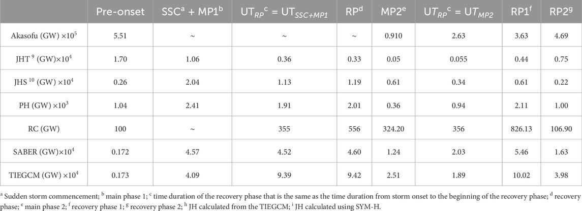
Table 1. Total power input and dissipation during the 28 October–1 November 2003 storm.
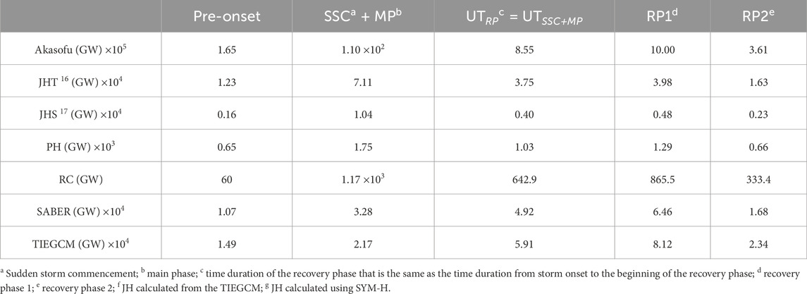
Table 2. Total power input and dissipation during the 19–22 November 2003 storm.
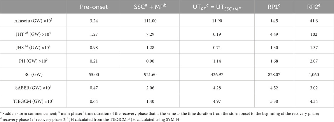
Table 3. Total power input and dissipation during the 6–10 November 2004 storm.
We investigate the thermospheric energy budget during the extreme geomagnetic storms (Dst
Figure 1 shows the (a) interplanetary magnetic field, (b) solar wind dynamic pressure and proton density, (c) solar wind speed, and (d) Dst/SYM-H index during the 28 October–01 November 2003 superstorm. The vertical dashed lines represent the onset time of the geomagnetic storm. This storm event is associated with two X-flares at approximately 11:10 UT on 28 October and 20:50 UT on 29 October 2003 and two large CMEs. The associated first CME resulted in the southward turning of the IMF Bz at approximately 6 UT on 29 November 2003, and correspondingly, the sudden storm commencement (SSC) can be noticed. The solar wind speed reached more than 2,000 km/s, which is one of the fastest solar winds ever directly measured in the space era (Skoug et al., 2004; Rosenqvist et al., 2005). The strong solar wind speed increased the proton temperature significantly higher than that observed during a typical CME storm (figure not shown). However, other parameters such as proton density and dynamic pressure were moderate. The SYM-H (Dst) index reached a minimum value of approximately −391 nT (−353 nT), which was observed more than 18 h after the storm onset (Figure 1D). The arrival of the second CME resulted in the southward movement of the IMF Bz at approximately 19 UT on 30 October 2003 with the solar wind speed exceeding 1,500 km/s. The proton density and the dynamic pressure reached the values of 15 cc−1 and 20 nPa, respectively. The southward turning of IMF Bz indicated the commencement of the storm at approximately 19 UT on 30 October 2003, which can be observed from the SYM-H/Dst index. The minimum value of the SYM-H (Dst) index was approximately −432 nT (−383 nT) at approximately 23 UT on 30 October 2003. The second storm was more geoeffective and resulted in larger re-intensification than the first storm, considering the low value of the SYM-H/Dst index (Rosenqvist et al., 2005).
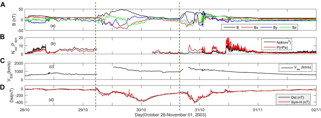
Figure 1. Solar wind variation during the 28 October–1 November 2003 storm. (A) Interplanetary magnetic field (Bx, By, and Bz), (B) proton density and dynamic pressure, (C) solar wind speed, and (D) Dst and SYM-H indexes. The vertical blue dashed lines represent the onset time of the storm.
The temporal variation in the corresponding energy input and dissipation during the 28 October–1 November 2003 storm is shown in Figure 2. It depicts the (a) Akasofu parameter, (b) Joule heating, auroral particle heating, and ring current power, and (c) orbit averaged NO cooling flux. The energy input and dissipation are calculated using the empirical formulations, as discussed above. The NO cooling fluxes are obtained from the TIMED-SABER satellite and the TIEGCM simulations. The vertical dashed blue lines represent the time of onset, recovery, and the time 24 h prior to onset. The vertical red dashed lines represent the time duration of the recovery phase (UTRP) that is same as the time duration from the storm onset to the beginning of the recovery phase (UTRP = UTonset + UTMP; MP = main phase). The unavailability of solar wind data during 29 October and most of 30 October 2003 makes it difficult to understand the temporal evolution of the Akasofu parameter during 29–30 October 2003. A significant enhancement in the Akasofu parameter occurred during the second storm (storm 2, 30 October) within 2–3 h of the commencement of the storm, reaching the maximum value of 2.5 × 10⁴ GW.
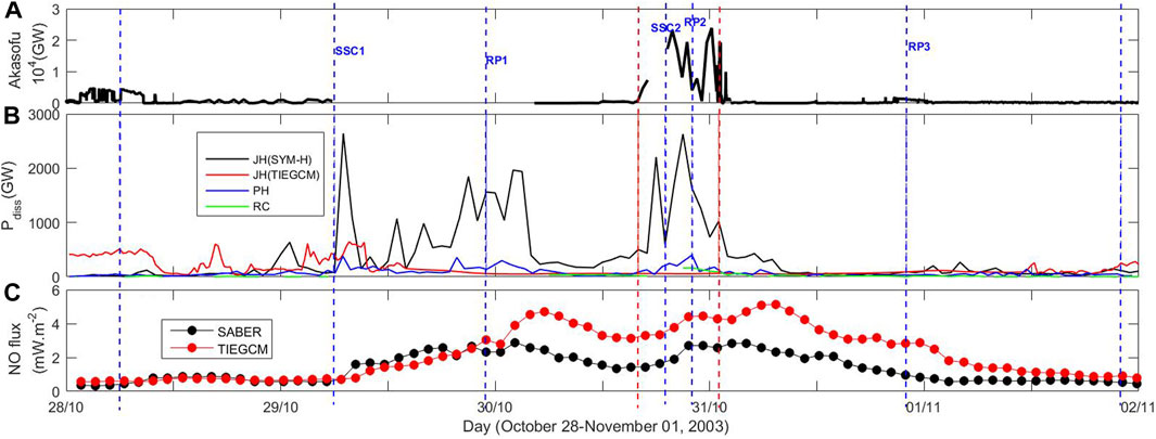
Figure 2. Time variation in the energy distribution during the 28 October–01 November 2003 storm. (A) Akasofu parameter, (B) Joule heating power from hourly SYM-H (black) and TIEGCM (red) observations, particle heating (blue) and ring current (green), and (C) orbit averaged NO cooling flux from SABER observations (black) and the TIEGCM simulation (red). The vertical blue dashed lines represent the time of onset–24 h, onset, recovery, and recovery + 24 h. The vertical red dashed lines represent the time of recovery that is the same as the duration of onset + main phase.
The response of the thermospheric Joule heating, auroral particle precipitation, and the ring current dissipation to the solar energy deposition is shown in Figure 2B. The Joule heating power, calculated using the SYM-H index, shows a sharp increase during 29–30 October 2003 with significant temporal fluctuations (hereafter, JHS denotes Joule heating calculated using hourly averaged SYM-H and PC and JHT denotes Joule heating from the TIEGCM). On the other hand, the global JHT does not show any appreciable enhancement. It can be attributed to the unreliable solar wind data during this period and subsequent calculation of the high-latitude electric field using the Weimer model. The Weimer model takes solar wind density, solar wind speed, and interplanetary magnetic fields (IMF By and IMF Bz) as the input parameters. Although the ion convection pattern and the cross polar cap potential (CPCP) are sensitive to IMF By, IMF Bz, and solar wind speed in the Weimer model, the CPCP is relatively insensitive to the solar wind density. In addition, the Weimer model can result in erroneous output, such as the electric potential patterns, for solar wind speed exceeding 900 km/s and IMF
The time history of the (a) interplanetary magnetic field, (b) proton density and dynamic pressure, (c) solar wind speed, and (d) Dst and SYM-H indices during 19–22 November 2003 storm is shown in Figure 3. The halo CMEs and associated M-class solar flares on 18 October 2003 triggered the strongest storm of solar cycle#23 (Srivastava, 2005). The IMF Bz turned southward at 08 UT on 20 November 2003 that reached a minimum value of −50 nT on the same day. The vertical blue line represents the onset of the storm. The proton density, dynamic pressure, and solar wind speed attained maximum values of 30 cc−1, 25 nPa, and 750 km/s, respectively. The SYM-H (Dst) index decreased for approximately 11 h, reaching a minimum value of −490 (−473) nT at approximately 19 UT on 20 November 2003, followed by a long recovery phase.
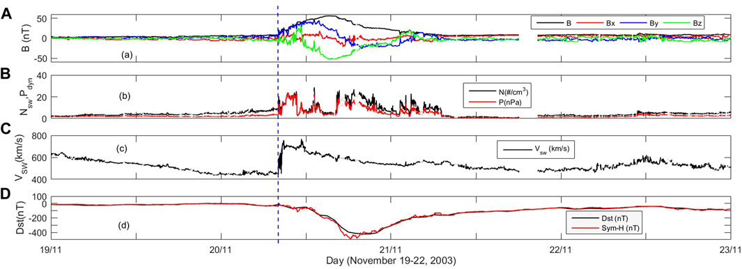
Figure 3. Solar wind variation during the 19–22 November 2003 storm. (A) Interplanetary magnetic field (Bx, By, and Bz), (B) proton density and dynamic pressure, (C) solar wind speed, and (D) Dst and SYM-H indexes. The vertical blue dashed line indicates the onset of the storm.
The temporal variation in the (a) Akasofu parameter; (b) Joule heating, auroral particle precipitation, and ring current power; and (c) orbit averaged NO cooling flux during 19–22 November 2003 storm is shown in Figure 4. The Akasofu parameter shows a sharp increase with small temporal fluctuation as the storm starts. It takes approximately 7–8 h for the solar wind to transfer its maximum energy to the magnetosphere. The maximum calculated value of the Akasofu parameter is approximately 3.6 × 10⁴ GW. In response to the solar wind energy input, the JHS increased to 1,650 GW at approximately 20 UT on 20 November 2003. A significant enhancement is observed in the JHT. This value (2,850 GW) is about 60% higher than the JHS. In addition, it can be observed that the JHT exhibits both the faster enhancement and recovery. Nonetheless, peak Joule heating power is obtained almost at the same time. The auroral particle precipitation (maximum of 200 GW) and the ring current power (maximum of 180 GW) also increased almost at the same time. The thermospheric cooling flux, obtained from the TIEGCM simulations and SABER observations, increased as the storm intensified. Both the model and observations peak at approximately 2 UT on 21 November 2003, almost 20 h after the storm onset. The maximum NO cooling power lags by approximately 8–10 h to the peak Joule heating power. However, it can be observed that the satellite observation responds faster than the model simulation.
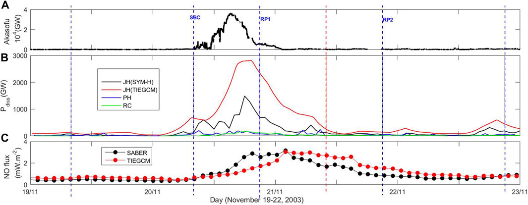
Figure 4. Time variation in the energy distribution during the 19–22 November 2003 storm. (A) Akasofu parameter, (B) Joule heating power from SYM-H (black) and the TIEGCM (red), particle heating (blue), and ring current (green), and (C) orbit averaged NO cooling flux from SABER observations (black) and the TIEGCM simulation (red). The vertical blue dashed lines represent the time of onset–24 h, onset, recovery, recovery + 24 h, and recovery + 48 h. The vertical red dashed line represents the time of recovery that is the same as the duration of onset + main phase.
Figure 5 shows the interplanetary data and SYM-H/Dst index for the storm period 6–10 November 2004. It resulted due to a series of solar events that occurred during 4 November 2004 (Yermolaev et al., 2008). The solar wind shock reached Earth at approximately 10 UT on 7 November 2004. Because of it, the y-and z-components of the interplanetary magnetic field started to oscillate until approximately 23 UT. The IMF Bz remained southward for most of the period during 7–10 November (Figure 5A). The IMF By and Bz showed strong negative values of approximately 50 nT. The proton density and dynamic pressure increased abruptly. The solar wind speed remained elevated (
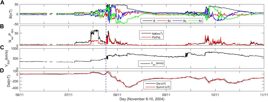
Figure 5. Solar wind variation during the 6–10 November 2004 storm. (A) Interplanetary magnetic field (Bx, By, and Bz), (B) proton density and dynamic pressure, (C) solar wind speed, and (D) Dst and SYM-H indexes. The vertical blue dashed line represents the onset time of the storm.
Figure 6 shows the solar energy input and dissipation during 6–10 November 2004. The Akasofu parameter is shown in Figure 6A. As the storm commenced, a sudden increase in the Akasofu parameter within 1–2 h can be observed with maximum solar wind energy deposition into the magnetosphere occurring within 5–10 h of onset. The empirically calculated Joule heating power exhibits a temporal fluctuation (Figure 6B). The JHT shows a more smooth variation with a maximum value of approximately 3,000 GW at approximately 4 UT on 8 November 2004. The maximum JHS of 1,680 GW, 1,800 GW, and 1,910 GW are obtained at approximately 02 UT, 04 UT, and 06 UT on 8 November 2004, respectively. In addition, it can be observed that the Joule heating power during the recovery phase is comparable to that during the main phase, although the storm is less intense. The maximum JHS is approximately 2,600 GW at 21 UT on 9 November 2003, whereas it is approximately 1,500 GW for JHD, which peaks approximately 2 h later. The auroral particle heating and ring current dissipation also increase during the storm period (Figure 6B). The auroral particle heating (280 GW) is maximum at approximately 06 UT on 8 November 2004, whereas the ring current power (150 GW) is maximum at approximately 02–03 UT on 7 November 2004. The kinetic energy, Akasofu parameter, and the thermospheric/ionospheric dissipation of same orders have been reported earlier (Alex et al., 2006; DeLucas et al., 2007). Figure 6C shows the temporal variation in the orbit averaged NO cooling fluxes, as observed by the TIMED-SABER satellite and the TIEGCM simulation. The model result is slightly higher than that observed during the magnetic quiet period. The average values of the model results and observations are approximately 0.22 mWm−2 and 0.12 mWm−2, respectively. When the storm started, the NO flux intensified. The satellite observation shows a stronger enhancement and a faster recovery than the model result. A peak satellite measurement of 2.9 mWm−2 is observed at 07 UT on 8 November 2004. The model result lags the observation by approximately 10 h with a slightly lower magnitude. The model result peaks at approximately 17 UT on the same day with a peak value of 2.5 mWm−2. It is to be noted that the SABER observation of the peak NO flux lags the peak Joule heating power by approximately 2–5 h. The increase in the modeled result is lower than that in the satellite observations. The SABER cooling flux increases by more than an order of magnitude compared to the pre-onset value, whereas the model result increases by about 800%. The counter-reaction of the NO flux to the intense storms during the recovery phase of 9–10 November, with both the observed and modeled results reviving, is shown in Figure 6D. The model result and the satellite observation increase by more than 30% and decrease by 10%, respectively, of their main phase 1 values. The peak values are approximately 3.5 mWm−2 and 2.8 mWm−2 for the model simulations and observations, respectively.
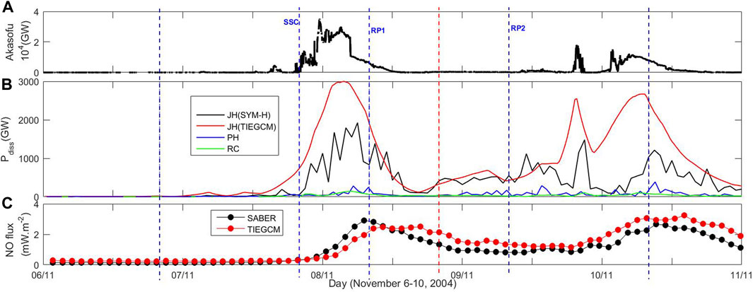
Figure 6. Time variation in the energy distribution during the 6–10 November 2004 storm. (A) Akasofu parameter, (B) Joule heating power from SYM-H (black) and the TIEGCM simulation (red), particle heating (blue), and ring current (green), and (C) orbit averaged NO cooling flux from SABER observations (black) and the TIEGCM simulation (red). The vertical blue dashed lines represent the time of onset–24 h, onset, recovery, recovery + 24 h, and recovery + 48 h. The vertical red dashed line represents the time of recovery that is the same as the duration of the onset + main phase.
The comparison of the energy distributions during the three geomagnetic storms mentioned above is shown in Figure 7. The top panels (Figures 7A–C) show the Dst and SYM-H indices. The vertical blue and red dashed lines indicate the time periods considered in calculating the total power. Although it is discussed in the previous sections and marked in the figure, we would like to mention it again. The left- and right-most vertical lines represent the 24 h prior to the onset and 24 h following recovery phase 1, respectively. The red dashed lines represent the time duration of the recovery phase (UTRP; RP = recovery phase) that is the same as the time duration from the storm onset to the beginning of the recovery phase (UTRP = UTonset + UTMP; MP = main phase). The corresponding energy distribution is enclosed within the red box. The bottom panels show the energy input into the thermosphere and thermospheric/ionospheric power dissipations. The total energy entering the magnetosphere and subsequent evolution of ionospheric/thermospheric energy dissipation during different phases of the 28 October–1 November 2003 geomagnetic storm are shown in Figure 7D. The solar wind data are not available from the onset of the storm on 29 October 2003 (storm 1) to some parts of the onset of the second storm on 30 October 2003 (storm 2). The Akasofu parameter shows a linear increase with the storm’s activity. However, it is unexpectedly high during pre-onset due to the elevated solar wind speed and proton density. The total values of the Akasofu parameter (9.1 × 10⁴ GW) are minimum during main phase 2, which lacks data during most of the period (the total value is the sum of the concerned parameter within the specified time duration). On the other hand, a maximum total Akasofu value (4.69 × 10⁵ GW) is observed during recovery phase 2. The higher value of the Akasofu parameter during storm 2 than during storm 1 can be attributed to the fact that the second storm was more geoeffective than the first storm (Rosenqvist et al., 2005). The Joule heating power, as calculated using hourly SYM-H (JHS), is lower during the pre-onset phase, whereas that obtained from the TIEGCM (JHT) is higher. The JHS showed a nonlinear variation with respect to the storm’s intensity. It increased by three times in magnitude during the main phase, reaching a maximum total value of 2.04 × 10⁴ GW that decreased as the storm progressed. Surprisingly, the total Joule heating power during the main phase of storm 2 is lower than that of storm 1, although storm 2 is stronger than storm 1. On the other hand, the JHT shows a decrease in storm 2 compared to storm 1. This surprising behavior can be attributed to the erroneous solar wind parameters and subsequent convection electric field calculation using the Weimer model. The auroral particle precipitation, during storm 1, shows a linear variation with the storm’s intensity with a maximum total value of 2.41 × 10³ GW observed during the main phase. The total auroral particle precipitation for storm 2 is minimum (356.6 GW) during the main phase of storm 2, which increases with the storm’s progression, and a total value of 2.113 × 10³ GW is achieved during recovery phase 1. Similar variation in the ring current injection power can also be observed with a minimum value during the recovery phase of storm 1. The total SABER observed and the total modeled cooling power are almost the same (
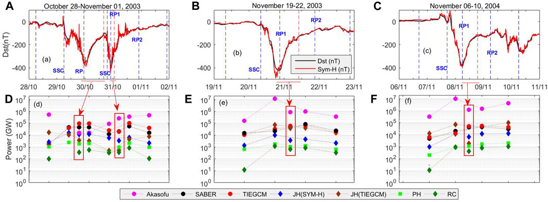
Figure 7. Top panels: Time variation in Dst and SYM-H indexes during (A) 28 October–1 November 2003, (B) 19–22 November 2003, and (C) 6–10 November 2004. Bottom panels: Energy propagation/dissipation during (D) 28 October–1 November 2003, (E) 19–22 November 2003, and (F) 6–10 November 2004. Magenta circle: Akasofu parameter; blue diamond: Joule heating power from SYM-H (JHS); violet diamond: Joule heating power from the TIEGCM (JHT); green square: auroral particle precipitation; green diamond: ring current; black circle: SABER-observed NO flux; red circle: TIEGCM-simulated NO flux. The parameters within the red box are during the time of recovery that is the same as the duration of the onset + main phase. SSC, sudden storm commencement; RP, recovery phase; RP1, recovery phase 1; RP2, recovery phase 2. See text for details.
The superstorms of 19–22 November 2003 (SYM-H = −490 nT) and the main phase 1 (SYM-H = −391 nT) of 28 October−1 November 2003 are, respectively, the strongest and weakest storms among all, as observed from the SYM-H index. Although the Joule heating power peaks during main phases of the storms, it does not strictly follow the storm’s intensity. Since the maximum Joule heating power is observed during the main phases, we particularly emphasize on the main phases of the storm as far as the Joule heating power is concerned. The maximum total (2.04 × 10⁴ GW) and minimum total (3.4 × 10³ GW) Joule heating powers, as calculated using SYM-H (JHS), are, respectively, found during main phase 1 (SYM-H = −391 nT) and main phase 2 (SYM-H = −432 nT) of the 28 October–1 November 2003 storm. Similarly, the JHT has a maximum total value of 7.3 × 10⁴ GW during 6–10 November 2004 (SYM-H = −395 nT) and minimum total value of 496 GW during main phase 2 of the 28 October–1 November 2003 storm (SYM-H = −432 nT). The magnitude of the Joule heating power depends on the method by which it is calculated. The total magnitude of the Akasofu parameter is 1.25 × 10⁷ GW and total JHT is 1.4 × 10⁵ GW during 19–22 November 2003. Similarly, they are, respectively, approximately 1.69 × 10⁷ GW and 2.88 × 10⁵ GW during 6–10 November 2004. It suggests that the Joule heating power during extreme storms accounts for about 1% of the energy input; less than a percent is available for the auroral ionosphere, which is in conformity with the results obtained by Vichare et al. (2005) and MacMahon and Gonzalez (1997) for intense storms. Note that earlier studies report an order of 10% fraction of energy input into the magnetosphere, which is dissipated via Joule heating and auroral power during intense storms (Guo et al., 2012; Turner et al., 2009; and references therein). Alex et al. (2006) reported that the Joule heating dissipation power, using the AE index as a proxy, accounted for about 4.5%, 4.9%, and 5.7% of energy input on 29 October, 30 October, and 20 November 2003, respectively. Note that the energy deposited into the magnetosphere via the formation of field-aligned current, magnetospheric tail current, energy carried away by the plasmoids, and the post-plasmoid plasma sheet outflow are not considered in the present study, which appear to be a major portion of energy dissipation (Alex et al., 2006; Baker et al., 2001). The large caveat observed in the present study can be attributed to the empirical formulations used.
The energy input is highly variable at a timescale of an hour, particularly during the main phase of the geomagnetic storm (Verkhoglyadova et al., 2017). The Epsilon (Akasofu) parameter can add to a significant amount of uncertainty, owing to the scale factor (see Koskinen and Tanskanen, 2002 for detailed discussion). The Joule heating power calculated using the formulation proposed by Knipp et al. (2004) is the multiple regression fit to the integrated Joule heating values derived from the assimilative mapping of ionospheric electrodynamics (AMIE). It is expected to have scarcity of data points at the extreme end of super geomagnetic storms. Furthermore, it does not include the neutral wind effects and small-scale variabilities of the electric field that considerably add to the Joule heating power (Knipp et al., 2004). The Joule heating power from the TIEGCM simulation, in the present study, uses high-latitude electric fields and convection patterns from the Weimer model (Weimer, 2005). The Weimer modeled Joule heating rate can be significantly different (about a factor of 2) from other calculations and is less sensitive to solar wind drivers (Verkhoglyadova et al., 2017; Huang et al., 2012). One of the limitations to the Weimer model is that it neglects the cups heating, and the electric potential patterns become unrealistic for high-speed solar wind (Vsw > 900 km/s) and high magnitude (
The total cooling power from SABER observation roughly follows the strength of the storm, with maximum values (6.4 × 10⁴ GW) during 19–22 November 2003 and minimum values (4.52 × 10⁴ GW) during 6–10 November 2004, whereas no similar variation is observed in the modeled power. The total modeled power is maximum during storm 2 of 28 October–1 November 2003 and minimum during 6–10 November 2004. The difference in the variation in cooling power with respect to the Joule heating power can be attributed to the different timescales used and the pre-conditioning of the thermosphere (Verkhoglyadova et al., 2016; Bag, 2018). The total power radiated by the NO cooling process is maximum during the 28 October−01 November 2003 storm, as calculated from the model (3.0 × 10⁵ GW) and satellite observation (1.8 × 10⁵ GW). Minimum radiative power is observed during 6–10 November 2004 for both the model (1.2 × 10⁵ GW) and satellite observation (1.0 × 10⁵ GW). The TIEGCM simulation predicts, on average, a power of 1.87 × 10⁵ GW exiting the thermosphere during a superstorm. It is about 40% higher than the satellite observation.
Figure 8 shows the scatter plot between the Akasofu parameter with (a) Joule heating power obtained from the TIEGCM, (b) Joule heating power calculated using SYM-H, (c) auroral particle precipitation, and (d) ring current dissipation power. It also displays the scatter plots during different geomagnetic storm phases. The Akasofu parameter exhibits a strong positive correlation with the Joule heating power (r = 0.75), as obtained from the TIEGCM simulation. A slightly lower correlation is observed for the Joule heating power calculated using SYM-H (r = 0.73), followed by ring current dissipation (r = 0.67). The auroral particle precipitation shows the lowest correlation with solar wind energy input into the magnetosphere. The higher correlation with the Joule heating could be due to the fact that it is by far the dominating dissipation process of energy input into the magnetosphere–ionosphere–thermosphere system (Kozyra et al., 1998; Lu et al., 1998) and that the nitric oxide cooling accounts for about 80% of Joule heating energy during geomagnetic storms (Lu et al., 2010).
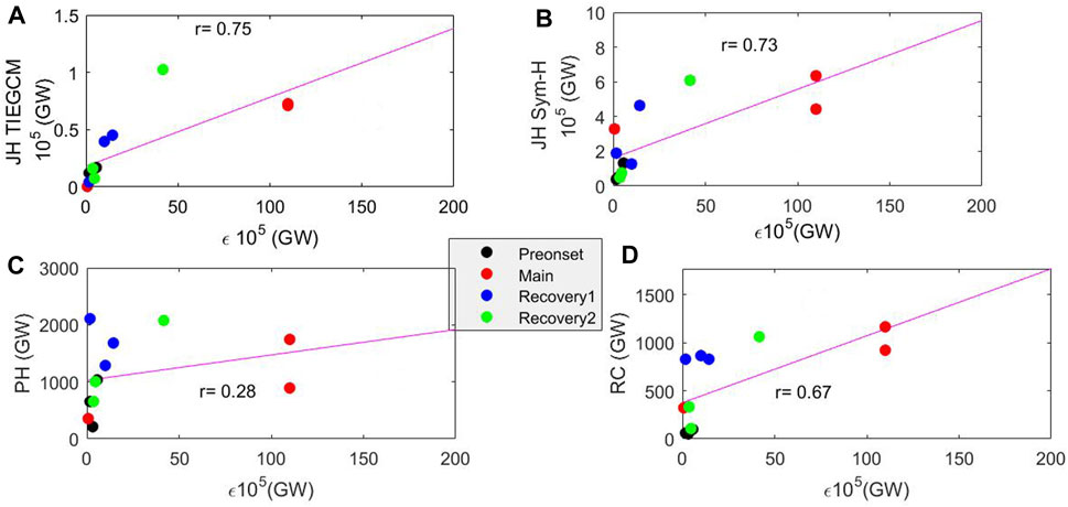
Figure 8. Scatter plot between the Akasofu parameter and (A) Joule heating power from the TIEGCM, (B) Joule heating power using SYM-H, (C) auroral particle precipitation, and (D) ring current power during different phases of geomagnetic storms.
The TIEGCM simulation agrees very well with the observations during the pre-onset period. The TIEGCM results increase higher than the observations during the geomagnetic period. Furthermore, the satellite observation exhibits a higher correlation (r = 0.35) with the Joule heating power calculated using SYM-H, where time lag is not considered (Figure 9A). A similar higher correlation can also be observed between the satellite-observed NO cooling power and the TIEGCM-simulated Joule heating power (Figure 9B). On the other hand, the TIEGCM simulated cooling power shows less correlation with the JHS and JHT (r = 0.10 for JHS and r = −0.16 for JHT), as shown in Figure9A–B. The consideration of time lag increases the correlation between the Joule heating and NO power (figure not shown). The correlation coefficient (r) is 0.76 for JHS and SABER observations, whereas it is about 0.75 for JHS and TIEGCM cooling flux. Furthermore, the correlation coefficient decreased significantly when the TIEGCM-simulated Joule heating rate (JHT) is used. The correlation coefficients are, respectively, 0.65 and 0.63 for JHT and SABER-observed flux and JHT and TIEGCM-calculated flux. These lower correlations, due to the inclusion of JHT, can be attributed to the unexpectedly low JHT during main phase 1 of the 28 October–1 November 2003 storm. The correlation coefficients, respectively, become 0.927 and 0.91 for JHT with SABER-observed flux, and JHT with TIEGCM-simulated flux when main phase 1 of the 28 October–1 November 2003 storm is excluded. These values agree very well with the earlier study by Lu et al. (2010). Lu et al. (2010) reported the cross-correlation coefficient, between NO cooling and the averaged, time-shifted Joule heating, in the range of 0.87–0.97 with a lag time of 10 h. The lower values of correlations between JHS and SABER-observed flux and JHS and TIEGCM flux could be due to the calculation of JHS using empirical formulation. The phase-wise correlation, between the NO cooling flux and Joule heating, shows a strong positive correlation (average r = 0.93) during the main phase (with the exclusion of main phase 1 of 28 October–1 November 2003), followed by recovery phase 1 (average r = 0.81).
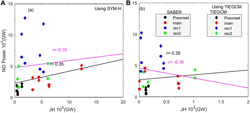
Figure 9. Scatter plot between (A) NO cooling power and Joule heating obtained using SYM-H and (B) NO cooling power and Joule heating obtained from the TIEGCM simulation (circle: SABER observation; diamond: TIEGCM simulation).
Figure 10 shows the correlation between the duration of the main phase with the modeled and satellite-observed NO power during the main phase (Figure 10A) and recovery phase (Figure 10B). Both the satellite observations and model simulations of cooling power demonstrate a strong positive correlation with correlation coefficients of 0.96 and 0.59, respectively, during the main phase. The satellite observations of cooling power show a relatively stronger negative correlation (r = −0.49) than the modeled power (r = −0.12) during the recovery phase. Discrepancies between the model simulations of NO cooling emission and the satellite observations have been reported earlier during intense storms (Sheng et al., 2017; Chen and Lei, 2018; Li et al., 2019; Walterscheid et al., 2023). It suggests that the observation displays a faster response and faster recovery during extreme geomagnetic storms.
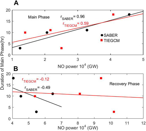
Figure 10. Scatter plot between the phase duration and NO cooling power calculated using SYM-H during the (A) main phase and (B) recovery phase.
We selected three superstorms with a Dst index less than −350 nT to study the thermospheric energy budget during 2003–2004. A particular consideration is given to the thermospheric cooling emission by nitric oxide via a wavelength of 5.3 μm because of its well-known thermostat effect. The nitric oxide radiative emission data are obtained from SABER observations onboard the TIMED satellite and the TIEGCM simulations. Different energy sources for magnetospheric energy injection and the thermospheric dissipation processes are calculated using space-borne and ground-based measurements and empirical formulations. The kinetic energy impinging on Earth’s magnetosphere, Joule heating, and the ring current injection rate are calculated using empirical formulations and TIEGCM simulations. The Akasofu parameter, which represents the solar wind energy transfer into Earth’s magnetosphere, is obtained from the SuperMAG database for two events and estimated for one event (28 October–1 November 2003). The auroral particle precipitation is from the DMSP F13 satellite. The nitric oxide volume emission rates, in the altitude region of 100–250 km, are integrated to obtain the cooling flux. The cooling flux is then integrated zonally and meridionally to estimate the nitric oxide cooling power exiting the thermosphere. The salient features obtained from this investigation are as follows: (I) the TIMED/SABER satellite observed that nitric oxide cooling flux responds faster to the solar wind energy input than that by the TIEGCM simulation; (II) the nitric oxide cooling power increases by an order of magnitude during storm time, with respect to the pre-onset value, with maximum power radiated during the recovery phase; (III) the Joule heating rates calculated from different sources show similar temporal variations with significant difference in the magnitude; (IV) the cooling power strongly depends on the duration of the storm main phase and is independent of the storm’s intensity; (V) the TIMED/SABER satellite observations show that, on average, nitric oxide cooling power of 1.4 × 10⁵ GW exits the thermosphere during a typical superstorm, which is about 40% less than that predicted by the TIEGCM simulation.
Publicly available datasets were analyzed in this study. The thermospheric nitric oxide cooling data from the TIMED-SABER satellite are available at http://saber.gats-inc.com/data.php and those from TIEGCM are available at the CCMC webpage (https://ccmc.gsfc.nasa.gov/;Run: TB_061923_IT_4, aswinithampi_sl_091722_IT_3 and TB_102023_IT_1). The DMSP satellite data are obtained from the Institute for Scientific Research, Boston College. Solar wind and magnetic data are from NASA’s OmniWeb (https://omniweb.gsfc.nasa.gov/). The Akasofu coupling function is from SuperMAG (https://supermag.jhuapl.edu/), last accessed on 15 December 2022).
TB: conceptualization, data curation, formal analysis, funding acquisition, investigation, methodology, resources, software, validation, visualization, writing–original draft, and writing–review and editing. RK: investigation, methodology, supervision, and writing–review and editing. YO: funding acquisition, investigation, methodology, project administration, resources, supervision, and writing–review and editing. HF: investigation, methodology, supervision, and writing–review and editing. ZL: investigation, methodology, and writing–review and editing. VS: methodology, supervision, writing–review and editing, and investigation. VS: methodology and writing–review and editing. SS: methodology, supervision, and writing–review and editing. PP: investigation, methodology, and writing–review and editing. ST: investigation, methodology, and writing–review and editing.
The author(s) declare that financial support was received for the research, authorship, and/or publication of this article. TB was supported by the Japan Society for the Promotion of Science (JSPS) postdoctoral fellowship for research in Japan, grant number 22F32017.
The authors thank the SABER, Community Coordinated Modeling Center (CCMC), DMSP, SuperMAG, and OmniWeb team for providing the data. TB was supported by the Japan Society for the Promotion of Science (JSPS) postdoctoral fellowship for research in Japan, grant number 22F32017. TB thanks M. Mlynczak for useful discussion. The authors thank Kevin Martin for providing the DMSP data.
The authors declare that the research was conducted in the absence of any commercial or financial relationships that could be construed as a potential conflict of interest.
All claims expressed in this article are solely those of the authors and do not necessarily represent those of their affiliated organizations, or those of the publisher, the editors, and the reviewers. Any product that may be evaluated in this article, or claim that may be made by its manufacturer, is not guaranteed or endorsed by the publisher.
Akasofu, S.-I. (1981). Energy coupling between the solar wind and the magnetosphere. Space Sci. Rev. 28, 121. doi:10.1007/bf00218810
Alex, S., Mukherjee, S., and Lakhina, G. S. (2006). Geomagnetic signatures during the intense geomagnetic storms of 29 October and 20 November 2003. J. Atmos. Sol.-Terr. Phys. 68 (7), 769–780. doi:10.1016/j.jastp.2006.01.003
Alexeev, I. I., Belenkaya, E. S., Kalegaev, V. V., Feldstein, Y. I., and Grafe, A. (1996). Magnetic storms and magnetotail currents. J. Geophys. Res. 101, 7737–7747. doi:10.1029/95ja03509
Bag, T. (2018). Diurnal variation of height distributed nitric oxide radiative emission during november 2004 super-storm. J. Geophys. Res.-Space Phys. 123, 6727–6736. doi:10.1029/2018ja025239
Bag, T., Li, Z., and Rout, D. (2021). SABER observation of storm-time hemispheric asymmetry in nitric oxide radiative emission. J. Geophys. Res. Space Phys. 126, e2020JA028849. doi:10.1029/2020JA028849
Bag, T., Rout, D., Ogawa, Y., and Singh, V. (2023a). Distinctive response of thermospheric cooling to ICME and CIR-driven geomagnetic storms. Astron. Space Sci. 10. doi:10.3389/fspas.2023.1107605
Bag, T., Rout, D., Ogawa, Y., and Singh, V. (2023b). Thermospheric NO cooling during an unusual geomagnetic storm of 21-22 January 2005: a comparative study between TIMED/SABER measurements and TIEGCM simulations. Atmos 14, 556. doi:10.3390/atmos14030556
Bag, T., Sunil Krishna, M., Gahlot, S., and Singh, V. (2014). Effect of severe geomagnetic storm conditions on atomic oxygen greenline dayglow emission in mesosphere. Adv. Space Res. 53 (8), 1255–1264. doi:10.1016/j.asr.2014.01.031
Baker, D. (2000). Effects of the sun on the Earth’s environment. J. Atmos. Sol.-Terr. Phys. 62 (17-18), 1669–1681. doi:10.1016/s1364-6826(00)00119-x
Baker, D. N., Daly, E., Daglis, I., Kappenman, J. G., and Panasyuk, M. (2004). Effects of space weather on Technology infrastructure. Space weather. 2. doi:10.1029/2003SW000044
Baker, D. N., Turner, N., and Pulkkinen, T. (2001). Energy transport and dissipation in the magnetosphere during geomagnetic storms. J. Atmos. Sol.-Terr. Phys. 63, 421–429. doi:10.1016/s1364-6826(00)00169-3
Barth, C. A. (1992). Nitric oxide in the lower thermosphere. Planet. Space Sci. 40, 315–336. doi:10.1016/0032-0633(92)90067-x
Bharti, G., Sunil Krishna, M. V., Bag, T., and Jain, P. (2018). Storm time variation of radiative cooling by nitric oxide as observed by TIMED-SABER and GUVI. J. Geophys. Res. Space Phys. 123 (2), 1500–1514. doi:10.1002/2017ja024576
Burton, R. K., McPherron, R. L., and Russell, C. T. (1975). An empirical relationship between interplanetary conditions and Dst. J. Geophys. Res. 80, 4204–4214. doi:10.1029/ja080i031p04204
Chen, G., Xu, J., Wang, W., and Burns, A. G. (2014). A comparison of the effects of CIR- and CME-induced geomagnetic activity on thermospheric densities and spacecraft orbits: statistical studies. J. Geophys. Res. 119, 7928–7939. doi:10.1002/2014ja019831
Chen, X., and Lei, J. (2018). A numerical study of the thermospheric over cooling during the recovery phases of the October 2003 storms. J. Geophys. Res. Space Phys. 123, 5704–5716. doi:10.1029/2017ja025120
De Lucas, A., Gonzalez, W., Echer, E., Guarnieri, F., Dal Lago, A., da Silva, M., et al. (2007). Energy balance during intense and super-intense magnetic storms using an Akasofu ϵ parameter corrected by the solar wind dynamic pressure. J. Atmos. Sol-Terr. Phys. 69 (15), 1851–1863. doi:10.1016/j.jastp.2007.09.001
Dessler, A. J., and Parker, E. N. (1959). Hydromagnetic theory of geomagnetic storms. J. Geophys. Res. 64, 2239–2252. doi:10.1029/jz064i012p02239
Dungey (1961). Interplanetary magnetic field and the auroral zones. Phys. Rev. Lett. 6, 47–48. doi:10.1103/physrevlett.6.47
Eastwood, J. P., Nakamura, R., Turc, L., Mejnertsen, L., and Hesse, M. (2017). The scientific foundations of forecasting magnetospheric space weather. Space Sci. Rev. 212, 1221–1252. doi:10.1007/s11214-017-0399-8
Ebihara, Y., and Ejiri, M. (2000). Simulation study on fundamental properties of the storm-time ring current. J. Geophys. Res. 105 (15), 15843–15859. doi:10.1029/1999ja900493
Ebihara, Y., Tanaka, T., and Kamiyoshikawa, N. (2019). New diagnosis for energy flow from solar wind to ionosphere during substorm: global MHD simulation. J. Geophys. Res. Space Phys. 124, 360–378. doi:10.1029/2018JA026177
Emery, B. A., Coumans, V., Evans, D. S., Germany, G. A., Greer, M. S., Holeman, E., et al. (2008). Seasonal, Kp, solar wind, and solar flux variations in long-term single-pass satellite estimates of electron and ion auroral hemispheric power. J. Geophys. Res. 113, A06311. doi:10.1029/2007ja012866
Emery, B. A., Roble, R. G., Ridley, E. C., Richmond, A. D., Knipp, D. J., Crowley, G., et al. (2012). Parameterization of the ion convection and the auroral oval in the NCAR thermospheric general circulation models. NCAR/TN-491+STR, HAO/NCAR. CO, United States: NCAR Technical Note.
Gardner, J. L., Lopéz-Puertas, M., Funke, B., Miller, S. M., Lipson, S. J., and Sharma, R. D. (2005). Rotational and Spin-orbit distributions of NO observed by MIPAS/ENVISAT during the solar storm of October/November 2003. J. Geophys. Res. 110, A09S34. doi:10.1029/2004ja010937
Guo, J., Feng, X., Emery, B. A., and Wang, Y. (2012). Efficiency of solar wind energy coupling to the ionosphere. J. Geophys. Res. 117, A07303. doi:10.1029/2012ja017627
Hagan, M. E., and Forbes, J. M. (2002). Migrating and nonmigrating diurnal tides in the middle and upper atmosphere excited by tropospheric latent heat release. J. Geophys. Res. 107, 4754. doi:10.1029/2001jd001236
Hajra, R., Echer, E., Tsurutani, B. T., and Gonzalez, W. D. (2014). Solar wind-magnetosphere energy coupling efficiency and partitioning: HILDCAAs and preceding CIR storms during solar cycle 23. J. Geophys. Res. Space Phys. 119, 2675–2690. doi:10.1002/2013JA019646
Heelis, R. A., Lowell, J. K., and Spiro, R. W. (1982). A model of the high-latitude ionospheric convection pattern. J. Geophys. Res. Space Phys. 87, 6339–6345. doi:10.1029/ja087ia08p06339
Horvath, I., and Lovell, B. C. (2010). Large-scale traveling ionospheric disturbances impacting equatorial ionization anomaly development in the local morning hours of the Halloween Superstorms on 29–30 October 2003. J. Geophys. Res. 115, A04302. doi:10.1029/2009JA014922
Huang, Y., Richmond, A. D., Deng, Y., and Roble, R. (2012). Height distribution of joule heating and its influence on the thermosphere. J. Geophys. Res. 117, A08334. doi:10.1029/2012JA017885
Hwang, E. S., Castle, K. J., and Dodd, J. A. (2003). Variational relaxation of NO(ν = 1) by oxygen atoms between 295 and 825 K. J. Geophys Res. 108, 1109. doi:10.1029/2002JA009688
Kamide, Y., Yokoyama, N., Gonzalez, W., Tsurutani, B. T., Daglis, I. A., Brekke, A., et al. (1998a). Two-step development of geomagnetic storms. J. Geophys. Res. 103 (A4), 6917–6921. doi:10.1029/97ja03337
Kamide, Y., Yokoyama, N., Gonzalez, W., Tsurutani, B. T., Daglis, I. A., Brekke, A., et al. (1998b). Two-step development of geomagnetic storms. J. Geophys. Res. 103 (A8), 6917–6921. doi:10.1029/97ja03337
Kataoka, R., Shiota, D., Fujiwara, H., Jin, H., Tao, C., Shinagawa, H., et al. (2022b). Unexpected space weather causing the re-entry of 38 Starlink satellites in February 2022. J. Space Weather Space Clim. 12, 41. doi:10.1051/swsc/2022034
Knipp, D., Kilcommons, L., Hunt, L., Mlynczak, M., Pilipenko, V., Bowman, B., et al. (2013). Thermospheric damping response to sheath-enhanced geospace storms. Geophys. Res. Lett. 40, 1263–1267. doi:10.1002/grl.50197
Knipp, D. J., Emery, B. A., Engebretson, M., Li, X., McAllister, A. H., Mukai, T., et al. (1998). An overview of the early November 1993 geomagnetic storm. J. Geophys. Res. 103, 26197–26220. doi:10.1029/98JA00762
Knipp, D. J., Pette, D. V., Kilcommons, L. M., Isaacs, T. L., Cruz, A. A., Mlynczak, M. G., et al. (2017). Thermospheric nitric oxide response to shock-led storms. Space weather. 15, 325–342. doi:10.1002/2016SW001567
Knipp, D. J., Tobiska, W. K., and Emery, B. A. (2004). Direct and indirect thermospheric heating sources for solar cycles 21-23. Sol. Phys. 224, 495–505. doi:10.1007/s11207-005-6393-4
Kockarts, G. (1980). Nitric oxide cooling in the terrestrial thermosphere. Geophys. Res. Lett. 7, 137–140. doi:10.1029/gl007i002p00137
Koskinen, H. E. J., and Tanskanen, E. (2002). Magnetospheric energy budget and the epsilon parameter. J. Geophys. Res. 107 (A11), 1415. doi:10.1029/2002JA009283
Kozyra, J. U., Crowley, G., Emery, B. A., Fang, X., Maris, G., Mlynczak, M. G., et al. (2006). “Response of the upper/middle atmosphere to coronal holes and powerful high-speed solar wind streams in 2003,” in Recurrent magnetic storms: corotating solar wind streams. Editors B. Tsurutani, R. McPherron, G. Lu, J. H. A. Sobral, and N. Gopalswamy (Hoboken, New Jersey, United States: Wiley). doi:10.1029/167GM24
Kozyra, J. U., Jordanova, V. K., Borovsky, J. E., Thomsen, M. F., Knipp, D. J., Evans, D. S., et al. (1998). Effects of a high-density plasma sheet on ring current development during the November 2-6, 1993, magnetic storm. J. Geophys. Res. 103 (A11), 26285–26305. doi:10.1029/98ja01964
Krauss, S., Temmer, M., and Vennerstrom, S. (2018). Multiple satellite analysis of the Earth’s thermosphere and interplanetary magnetic field variations due to ICME/CIR events during 2003-2015. J. Geophys. Res. 123, 8884–8894. doi:10.1029/2018JA025778
Krauss, S., Temmer, M., Veronig, A., Baur, O., and Lammer, H. (2015). Thermospheric and geomagnetic responses to interplanetary coronal mass ejections observed by ACE and GRACE: statistical results. J. Geophys. Res. 120, 8848–8860. doi:10.1002/2015JA021702
Lei, J., Burns, A. G., Thayer, J. P., Wang, W., Mlynczak, M. G., Hunt, L. A., et al. (2012). Overcooling in the upper thermosphere during the recovery phase of the 2003 October storms. J. Geophys. Res. 117, A03314. doi:10.1029/2011JA016994
Li, Z., Knipp, D., and Wang, W. (2019). Understanding the behaviors of thermospheric nitric oxide cooling during the 15 May 2005 geomagnetic storm. J. Geophys. Res.-Space Phys. 124, 2113–2126. doi:10.1029/2018JA026247
Li, Z., Knipp, D., Wang, W., Sheng, C., Qian, L., and Flynn, S. (2018). A comparison study of NO cooling between TIMED/SABER measurements and TIEGCM simulations. J. Geophys. Res.-Space Phys. 123, 8714–8729. doi:10.1029/2018JA025831
Liemohn, M. W., Kozyra, J. U., Jordanova, V. K., Khazanov, G. V., Thomsen, M. F., and Cayton, T. E. (1999). Analysis of early phase ring current recovery mechanisms during geomagnetic storms. Geophys. Res. Lett. 26, 2845–2848. doi:10.1029/1999gl900611
Lin, C. Y., and Deng, Y. (2019). Nitric oxide in climatological global energy budget during 1982–2013. J. Geophys. Res.-Space Phys. 124, 782–789. doi:10.1029/2018JA025902
Lin, C. Y., Deng, Y., Knipp, D. J., Kilcommons, L. M., and Fang, X. (2019). Effects of energetic electron and proton precipitations on thermospheric nitric oxide cooling during shock-led interplanetary coronal mass ejections. J. Geophys. Res.-Space Phys. 124, 8125–8137. doi:10.1029/2019JA027089
Liu, H., and Lühr, H. (2005). Strong disturbance of the upper thermospheric density due to magnetic storms: CHAMP observations. J. Geophys. Res. 110, A09S29. doi:10.1029/2004JA010908
Lu, G., Baker, D. N., McPherron, R. L., Farrugia, C. J., Lummerzheim, D., Ruohoniemi, J. M., et al. (1988). Global energy deposition during the January 1997 magnetic cloud event. J. Geophys. Res. Space Phys. 103 (A6), 11685–11694. doi:10.1029/98ja00897
Lu, G., Mlynczak, M. G., Hunt, L. A., Woods, T. N., and Roble, R. G. (2010). On the relationship of Joule heating and nitric oxide radiative cooling in the thermosphere. J. Geophys. Res. Space Phys. 115 (A5). doi:10.1029/2009ja014662
Lu, G., Richmond, A. D., Emery, B. A., and Roble, R. G. (1995). Magnetosphere-ionosphere thermosphere coupling: effect of neutral winds on energy transfer and field aligned current. J. Geophys. Res. Space Phys. 100 (A10), 19643–19659. doi:10.1029/95ja00766
MacMahon, R. M., and Gonzalez, W. D. (1997). Energetics during the main phase of geomagnetic superstorms. J. Geophys. Res. 102 (14), 14199–14207. doi:10.1029/97ja01151
Maeda, S., Fuller-Rowell, T. J., and Evans, D. S. (1989). Zonally averaged dynamical and compositional response of the thermosphere to auroral activity during September 18-24, 1984. J. Geophys. Res. 94 (A12), 16869–16883. doi:10.1029/JA094iA12p16869
Maeda, S., Fuller-Rowell, T. J., and Evans, D. S. (1992). Heat budget of the thermosphere and temperature variations during the recovery phase of a geomagnetic storm. J. Geophys. Res. 97 (A10), 14947–14957. doi:10.1029/92JA01368
Mannucci, A. J., Tsurutani, B. T., Iijima, B. A., Komjathy, A., Saito, A., Gonzalez, W. D., et al. (2005). Dayside global ionospheric response to the major interplanetary events of October 29-30, 2003 Halloween Storms. Geophys. Res. Lett. 32, L12S02. doi:10.1029/2004GL021467
Mannucci, A. J., Tsurutani, B. T., Kelley, M. C., Iijima, B. A., and Komjathy, A. (2009). Local time dependence of the prompt ionospheric response for the 7, 9, and 10 November 2004 superstorms. J. Geophys. Res. 114, A10308. doi:10.1029/2009ja014043
McComas, D., Bame, S. J., Barker, P. L., Delapp, D. M., Feldman, W. C., Gosling, J. T., et al. (1998). An unusual coronal mass ejection: first solar wind electron, proton, Alpha monitor (SWEPAM) results from the advanced composition explorer. Geophys. Res. Lett. 25, 4289–4292. doi:10.1029/1998gl900174
Mertens, C. J., Russell III, J. M., Mlynczak, M. G., She, C. Y., Schmidlin, F. J., Goldberg, R. A., et al. (2009). Kinetic temperature and carbon dioxide from broadband infrared limb emission measurements taken from the TIMED/SABER instrument. Adv. Space Res. 43, 15–27. doi:10.1016/j.asr.2008.04.017
Mlynczak, M., Martin-Torres, F. J., Russell, J., Beaumont, K., Jacobson, S., Kozyra, J., et al. (2003). The natural thermostat of nitric oxide emission at 5.3μm in the thermosphere observed during the solar storms of April 2002. Geophys. Res. Lett. 30 (21). doi:10.1029/2003GL017693
Mlynczak, M. G., Hunt, L. A., Thomas Marshall, B., Martin-Torres, F. J., Mertens, C. J., Russell, J. M., et al. (2010). Observations of infrared radiative cooling in the thermosphere on daily to multiyear timescales from the TIMED/SABER instrument. J. Geophys. Res. 115, A03309. doi:10.1029/2009ja014713
Mlynczak, M. G., Martin-Torres, F. J., Crowley, G., Kratz, D. P., Funke, B., Lu, G., et al. (2005). Energy transport in the thermosphere during the solar storms of April 2002. J. Geophys. Res. Space Phys. 110, A12. doi:10.1029/2005ja011141
Mlynczak, M. G., Martin-Torres, F. J., Marshall, B. T., Thompson, R. E., Williams, J., Turpin, T., et al. (2007). Evidence for a solar cycle influence on the infrared energy budget and radiative cooling of the thermosphere. J. Geophys. Res. 112, A02303. doi:10.1029/2006ja012194
Murphy, R. E., Lee, E. T. P., and Hart, A. M. (1975). Quenching of vibrationally excited nitric oxide by molecular oxygen and nitrogen. J. Chem. Phys. 63, 2919–2925. doi:10.1063/1.431701
National Science and Technology Council (2018). “Space weather phase 1 benchmarks,” in National science and technology (US) space weather operations, research and mitigation subcommittee (Washington, DC: Executive Office of the President of the United States).
Óbrien, T. P., and McPherron, R. L. (2000). An empirical phase space analysis of ring current dynamics: solar wind control of injection and decay. J. Geophys. Res. 105, 7707. doi:10.1029/1998JA000437
Oliveira, D. M., Zesta, E., Hayakawa, H., and Bhaskar, A. (2020). Estimating satellite orbital drag during historical magnetic superstorms. Space weather. 18 (11), e2020SW002472. doi:10.1029/2020SW002472
Oliveira, D. M., Zesta, E., Schuck, P. W., and Sutton, E. K. (2017). Thermosphere global time response to geomagnetic storms caused by coronal mass ejections. J. Geophys. Res. Space Phys. 122 (10), 10762–10782. doi:10.1002/2017JA024006
Palmroth, M., Janhunen, P., Pulkkinen, T. I., and Koskinen, H. E. J. (2004). Ionospheric energy input as a function of solar wind parameters: global MHD simulation results. Ann. Geophys. 22, 549–566. doi:10.5194/angeo-22-549-2004
Perreault, P., and Akasofu, S. I. (1978). A study of geomagnetic storms. Geophys. J. Int. 54, 547–573. doi:10.1111/j.1365-246x.1978.tb05494.x
Qian, L., Solomon, S. C., and Mlynczak, M. G. (2010). Model simulation of thermospheric response to recurrent geomagnetic forcing. J. Geophys. Res. 115, A10301. doi:10.1029/2010ja015309
Rich, F. J., Hardy, D. D., and Gussenhoven, M. S. (1985). Enhanced ionosphere-magnetosphere data from the DMSP satellites. EOS 66, 513–514. doi:10.1029/eo066i026p00513
Richards, P. G. (2004). On the increases in nitric oxide density at midlatitudes during ionospheric storms. J. Geophys. Res. 109, A06304. doi:10.1029/2003JA010110
Richmond, A. D., Ridley, E. C., and Roble, R. G. (1999). A thermosphere/ionosphere general circulation model with coupled electrodynamics. Geophys. Res. Lett. 19, 601–604. doi:10.1029/92gl00401
Roble, R. G., Ridley, E. C., Richmond, A. D., and Dickinson, R. E. (1988). A coupled thermosphere/ionosphere general circulation model. Geophys. Res. Lett. 15, 1325–1328. doi:10.1029/gl015i012p01325
Rosenqvist, L., Opgenoorth, H., Buchert, S., McCrea, I., Amm, O., and Lathuillere, C. (2005). Extreme solar-terrestrial events of October 2003: high-latitude and Cluster observations of the large geomagnetic disturbances on 30 October. J. Geophys. Res. 110, A09S23. doi:10.1029/2004ja010927
Sahai, Y., Fagundes, P. R., de Jesus, R., de Abreu, A. J., Crowley, G., Kikuchi, T., et al. (2011). Studies of ionospheric F-region response in the Latin American sector during the geomagnetic storm of 21-22 January 2005. Ann. Geophys. 29, 919–929. doi:10.5194/angeo-29-919-2011
Sarris, T. E., Talaat, E. R., Palmroth, M., Dandouras, I., Armandillo, E., Kervalishvili, G., et al. (2020). Daedalus: a low-flying spacecraft for in situ exploration of the lower thermosphere–ionosphere. Geoscientific Instrum. Methods Data Syst. 9 (1), 153–191. doi:10.5194/gi-9-153-2020
Sarris, T. E., Tourgaidis, S., Pirnaris, P., Baloukidis, D., Papadakis, K., Psychalas, C., et al. (2023). Daedalus MASE (mission assessment through simulation exercise): a toolset for analysis of in situ missions and for processing global circulation model outputs in the lower thermosphere-ionosphere. Front. Astron. Space Sci. 9, 1048318. doi:10.3389/fspas.2022.1048318
Schunk, R., and Nagy, A. (2009). Ionospheres: physics, plasma physics, and chemistry. Cambridge, United Kingdom: Cambridge University Press. doi:10.1017/CBO9780511635342
Sckopke, N. (1966). A general relation between the energy of trapped particles and the disturbance field near the earth. J. Geophys. Res. 71, 3125–3130. doi:10.1029/jz071i013p03125
Sheng, C., Lu, G., Solomon, S. C., Wang, W., Doornbos, E., Hunt, L. A., et al. (2017). Thermospheric recovery during the 5 April 2010 geomagnetic storm. J. Geophys. Res. Space Phys. 122, 4588–4599. doi:10.1002/2016ja023520
Sibeck, N., Lopez, R. E., and Roelof, E. C. (1991). Solar wind control of the magnetopause shape, location and motion. J. Geophys. Res. 96, 5489.
Sinnhuber, M., Nieder, H., and Wieters, N. (2012). “Energetic particle precipitation and the chemistry of the mesosphere/lower thermosphere,” in Crucial processes acting in the mesosphere/lower thermosphere. Editors E. Becker, and M. Rycroft (Berlin, Germany: Springer), 1281–1334.
Skoug, R. M., Gosling, J. T., Steinberg, J. T., McComas, D. J., Smith, C. W., Ness, N. F., et al. (2004). Extremely high-speed solar wind: 29-30 October 2003. J. Geophys. Res. 109, A9. doi:10.1029/2004ja010494
Smith, C. W., L’Heureux, J., Ness, N. F., Acuña, M. H., Burlaga, L. F., and Scheifele, J. (1998). The ACE magnetic fields experiment. Space Sci. Rev. 86, 613–632. doi:10.1007/978-94-011-4762-0_21
Srivastava, N. (2005). Predicting the occurrence of super-storms. Ann. Geophys. 23, 2989–2995. doi:10.5194/angeo-23-2989-2005
Sutton, E. K., Forbes, J. M., and Nerem, R. S. (2005). Global thermospheric neutral density and wind response to the severe 2003 geomagnetic storms from CHAMP accelerometer data. J. Geophys. Res. 110, A09S40. doi:10.1029/2004JA010985
Tang, C., Wei, Y., Liu, D., Luo, T., Dai, C., and Wei, H. (2017). Global distribution and variations of NO infrared radiative flux and its responses to solar activity and geomagnetic activity in the thermosphere. J. Geophys. Res. Space Phys. 122 (12), 534–612. doi:10.1002/2017JA024758
Tanskanen, E., Pulkkinen, T. I., Koskinen, H. E. J., and Slavin, J. A. (2002). Substorm energy budget during low and high solar activity: 1997 and 1999 compared. J. Geophys. Res. 107 (A6), 1086. doi:10.1029/2001JA900153
Troshichev, O. A., Kotikov, A. L., Bolotinskaya, B. D., and Andrezen, V. G. (1986). Influence of the IMF azimuthal component on magnetospheric substorm dynamics. J. Geomag. Geoelectr. 38, 1075–1088. doi:10.5636/jgg.38.1075
Tsurutani, B. T., and Gonzalez, W. D. (1994). The causes of geomagnetic storms during solar maximum. Eos Trans. AGU 75, 49–53. doi:10.1029/94eo00468
Tsurutani, B. T., Gonzalez, W. D., Tang, F., Akasofu, S. I., and Smith, E. J. (1988). Origin of interplanetary southward magnetic fields responsible for major magnetic storms near solar maximum (1978-1979). J. Geophys. Res. 93 (A8), 8519–8531. doi:10.1029/ja093ia08p08519
Turner, N. E., Baker, D. N., Pulkkinen, T. I., Roeder, J. L., Fennell, J. F., and Jordanova, V. K. (2001). Energy content in the storm time ring current. J. Geophys. Res. 106 (19), 19149–19156. doi:10.1029/2000ja003025
Turner, N. E., Cramer, W. D., Earles, S. K., and Emery, B. A. (2009). Geoefficiency and energy partitioning in CIR-driven and CME-driven storms. J. Atmos. Sol.-Terr. Phys. 71 (10-11), 1023–1031. doi:10.1016/j.jastp.2009.02.005
Valdivia, J. A., Sharma, A. S., and Papadopoulos, K. (1996). Prediction of magnetic storms by nonlinear models. Geophys. Res. Lett. 23, 2899–2902. doi:10.1029/96gl02828
Verkhoglyadova, O., Meng, X., Mannucci, A. J., Tsurutani, B. T., Hunt, L. A., Mlynczak, M. G., et al. (2016). Estimation of energy budget of ionosphere-thermosphere system during two CIR-HSS events: observations and modeling. J. Space Weather. Space Clim. 6, A20. doi:10.1051/swsc/2016013
Verkhoglyadova, O. P., Mannucci, A. J., Tsurutani, B. T., Mlynczak, M. G., Hunt, L. A., Redmon, R. J., et al. (2015). Localized thermosphere ionization events during the high-speed stream interval of 29 April to 5 May 2011. J. Geophys. Res. Space Phys. 120, 675–696. doi:10.1002/2014JA020535
Verkhoglyadova, O. P., Meng, X., Mannucci, A. J., Mlynczak, M. G., Hunt, L. A., and Lu, G. (2017). Ionosphere thermosphere energy budgets for the ICME storms of March 2013 and 2015 estimated with GITM and observational proxies. Space weather. 15, 1102–1124. doi:10.1002/2017SW001650
Vichare, G., Alex, S., and Lakhina, G. S. (2005). Some characteristics of intense geomagnetic storms and their energy budget. J. Geophys. Res. 110, A03204. doi:10.1029/2004JA010418
Vichare, G., Ridley, A., and Yiğit, E. (2012). Quiet-time low latitude ionospheric electrodynamics in the non-hydrostatic global ionosphere-thermosphere model. J. Atmos. Sol. Terr. Phys. 80, 161–172. doi:10.1016/j.jastp.2012.01.009
Walterscheid, R. L., Chen, M. W., Chao, C., Gegenheimer, S., Cabrera-Guzman, J., and McVey, J. (2023). Comparative accuracies of models for drag prediction during geomagnetically disturbed periods: a first principles model versus empirical models. Space weather. 21, e2022SW003332. doi:10.1029/2022SW003332
Wanliss, J., and Showalter, K. (2006). High-resolution global storm index: Dst versus SYM-H. J. Geophys. Res. 111, A02202. doi:10.1029/2005JA011034
Weimer, D. (2005). Predicting surface geomagnetic variations using ionospheric electrodynamic models. J. Geophys. Res. 110, A12307. doi:10.1029/2005ja011270
Weiss, L. A., Reiff, P. H., Moses, J. J., Heelis, R. A., and Moore, B. D. (1992). “Energy dissipation in substorms,” in Substorms 1, ESA SP-335 (Paris: Eur. Space Agency), 309–317.
Yee, J. H., Talaat, R., Christensen, A. B., Killeen, T. L., Russell, J. M., and Woods, T. N. (2003). TIMED instruments. Baltimore, Maryland, United States: Johns Hopkins APL Tech. Dig., 156–164.
Yermolaev, Yu I., Zelenyi, L., Kuznetsov, V., Chertok, I., Panasyuk, M., Myagkova, I., et al. (2008). Magnetic storm of November, 2004: solar, interplanetary, and magnetospheric disturbances. J. Atmos. Sol.-Terr. Phys. 70 (2-4), 334–341. doi:10.1016/j.jastp.2007.08.020
Keywords: extreme geomagnetic storm, thermospheric cooling power, nitric oxide emission, TIMED-SABER satellite observations, TIEGCM simulations
Citation: Bag T, Kataoka R, Ogawa Y, Fujiwara H, Li Z, Singh V, Sivakumar V, Sridharan S, Pirnaris P and Tourgaidis T (2024) Thermospheric nitric oxide energy budget during extreme geomagnetic storms: a comparative study. Front. Astron. Space Sci. 11:1273079. doi: 10.3389/fspas.2024.1273079
Received: 05 August 2023; Accepted: 23 April 2024;
Published: 15 May 2024.
Edited by:
Katya Georgieva, Bulgarian Academy of Sciences (BAS), BulgariaReviewed by:
Gaurav Bharti, Maa Shakumbhari University, IndiaCopyright © 2024 Bag, Kataoka, Ogawa, Fujiwara, Li, Singh, Sivakumar, Sridharan, Pirnaris and Tourgaidis. This is an open-access article distributed under the terms of the Creative Commons Attribution License (CC BY). The use, distribution or reproduction in other forums is permitted, provided the original author(s) and the copyright owner(s) are credited and that the original publication in this journal is cited, in accordance with accepted academic practice. No use, distribution or reproduction is permitted which does not comply with these terms.
*Correspondence: Tikemani Bag, dGlrZW1hbmkuYmFnQG5pcHIuYWMuanA=
Disclaimer: All claims expressed in this article are solely those of the authors and do not necessarily represent those of their affiliated organizations, or those of the publisher, the editors and the reviewers. Any product that may be evaluated in this article or claim that may be made by its manufacturer is not guaranteed or endorsed by the publisher.
Research integrity at Frontiers
Learn more about the work of our research integrity team to safeguard the quality of each article we publish.