Evaluation of the astrometric capability of Multi-Channel Imager and simulated calculation of proper motion of M31

Introduction: The Multi-Channel Imager (MCI), one of the back-end modules of the future China Space Station Telescope (CSST), is designed for high-precision spacebased astronomical observations. This paper evaluates the astrometric capability of the MCI based on simulated observational images and Gaia data: the M31 galaxy is selected as a representative case to validate the astrometric capability by calculating the proper motions (PMs) of the M31 member stars.

Method: We analyze the stellar centroids of the simulated images in the R, I and G bands, positional uncertainty of 2.5 mas for brighter foreground reference stars from the Gaia DR3 catalog and of 7.5 mas for the fainter M31 member stars, are adopted respectively. The theoretical PMs are generated from the adopted velocity field model, rotation curve, and stellar surface density profile. And the simulated observed PMs are generated from the aforementioned position uncertainties and theoretical PMs.

Result: We conclude that the precision of the MCI derived PMs strongly depends on the number of astrometric epochs per year. Specifically, uncertainty of 10 μas/yr is achievable with 10 epochs per year, and of 5 μas/yr with 50 epochs ignoring possible systematic effects. And symmetrically distributed observed fields yield better M31 kinematic parameters.

Discussion: Unknown systematic errors, space environment effects on detectors, dithering strategies, and observation schedules can affect the PMs of M31, the above issues need further analysis and validation in future work.

1 Introduction

The 2-m aperture China Space Station Telescope (CSST) is a large astronomical space telescope of China’s manned space program with a wide field of view, FoV (≥1.1 deg²) and high imaging quality (at λ = 0.633 μm, 80 of the energy of confined within a radius R_EE80 ≤ 0.15″ over FOV) (Zhan, 2011; Zhan, 2021). The CSST feeds multiple backend modules for diverse research tasks from solar system objects and exoplanets to cosmology. The Multi-Channel Imager (MCI) is one of these backend modules—a high-precision 3-channel in UV-visible simultaneous imaging camera. The main scientific objectives of MCI are (1) to carry out deep-field observations in the ultraviolet optical range and (2) to provide a higher-precision flux standard star catalog for the Chinese Space Station Optical Survey (CSS-OS) through high-precision photometry. The preliminary designed parameters of MCI are shown in Table 1:

TABLE 1

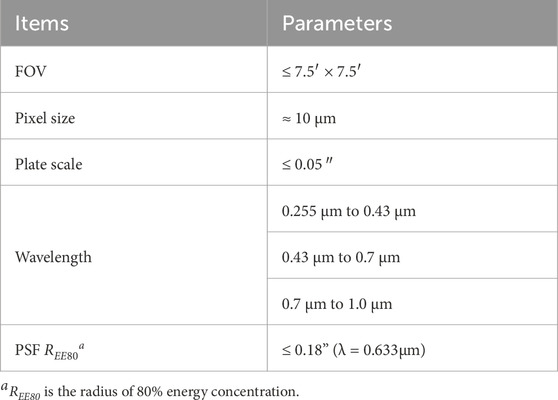
TABLE 1. Preliminary designed parameters of the MCI Instrument.

As seen, MCI has high-resolution and powerful detection capability. In addition to its applications in cosmology studies of Type Ia supernovae, strong gravitational lensing galaxy clusters, and joint evolution of galaxies and black holes, MCI can also be applied in high-precision astrometry such as PMs of external galaxies, parallax and PMs of brown dwarfs and the motion of galaxy jets. This paper takes calculation of PMs of Andromeda Galaxy (M31) to evaluate the astrometric capability of MCI. M31 is the largest spiral galaxy in the Local Group, located at a distance of 785 ± 25 kiloparsecs (kpc) from the Milky Way (MW), its RA (J2000) is 00h42m44.4s and Dec. (J2000) is +42°16′08″ (McConnachie et al., 2005; Chemin et al., 2009). The relative velocities between M31 and MW is one of the fundamental methods to provide a deeper understanding of the MW and the Local Group’s structure, formation, and evolution. The radial velocity of M31 has been accurately measured by Doppler spectroscopy: the heliocentric radial velocity is generally adopted as 301 ± 1 km/s and the velocity with respect to the LG center is generally −35 km/s (Karachentsev et al., 2004). The PM of M31 is small and challenging to measure. In optical astrometry, Hubble Space Telescope (HST) observations of three fields yielded $\left(\sigma {\mu }_{\alpha }*,\sigma {\mu }_{\delta }\right)$ (16.5, 15.4), (24.6, 24.4) and (27.8, 27.2) μas/yr (Sohn et al., 2012). More recently, Gaia DR2 yielded $\left(\sigma {\mu }_{\alpha }*,\sigma {\mu }_{\delta }\right)$ = (18, 15) μas/yr (van der Marel et al., 2019) and Gaia EDR3 – (10.7, 8.5) μas/yr (Salomon et al., 2021).

This paper first analyzes the astrometric measurement capability of MCI based on simulated observational images. It then takes the M31 as an example to assess the ability to calculate the PMs of M31 member stars by constructing simulated data. This paper is organized as follows. Section 2 describes the analysis of the astrometric capability of MCI by simulated images. Section 3 describes the M31 simulated data. Section 4 describes the method for the PM calculation. Section 5 presents the results and discussion. Summarizing the main results of the paper is presented in Section 6.

2 Evaluation of MCI astrometric capability

Using MCI simulated observational images in the u (central: 361.2 nm, FWHM: 80.4 nm), F555W (central: 526.7 nm, FWHM: 159.1 nm) and F814W (central: 833.8 nm, FWHM: 253.1 nm) bands to evaluate MCI’s astrometric capability, the analysis focuses on the relationship between the stellar astrometric measurement precision and magnitude. There are three steps in the simulation, first, calculating pixel coordinates (x, y) of the input catalog stars based on their celestial coordinates (α, δ) and telescope information. Second, generating simulated stars based on the Point Spread Function (PSF), stellar pixel coordinates, and magnitudes for each wavelength band. The simulated stellar PSF takes into account the mirror machining error, assembling error, gravity and thermal deformation error. After simulating wavefront aberration at different positions in the FOV, and then calculating the PSF, the PSF as shown in Figure 1B. Third, the dark current and its noise (0.00111e⁻pix⁻¹s⁻¹), readout noise (4e⁻), a wavelength dependent sky background and its noise (1.07 * 10^–19 to 1.07 * $\mathrm{1}{\mathrm{0}}^{-\mathrm{17}}{\mathrm{e}\mathrm{r}\mathrm{g}\mathrm{c}\mathrm{m}}^{-\mathrm{2}}{\mathrm{s}}^{-\mathrm{1}}{\mathring{\mathrm{A}}}^{-\mathrm{1}}{\mathrm{a}\mathrm{r}\mathrm{c}\mathrm{s}\mathrm{e}\mathrm{c}}^{-\mathrm{2}}$) were added to produce the simulated observational images (Yan, 2023). The bright-end stars (<22 mag) in the input synthetic catalog are taken from the Gaia DR3 catalog (Brown et al., 2021; Lindegren et al., 2021; Vallenari et al., 2023). The faint-end stars (>22 mag) are taken from the CSST-TRILEGAL catalog (Chen et al., 2023). Figure 1A shows a F555W band simulated image. The white square represents saturated star, due to each star occupies a 64 × 64 pixels region, the bright star exceeding this range is displayed as white square.

FIGURE 1

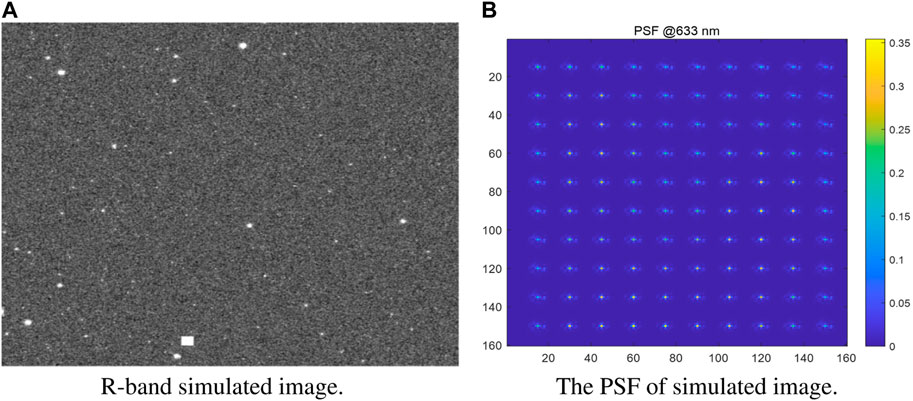
FIGURE 1. (A) F555W band simulated star image with a size of 9216 × 9232 pixels, corresponding to a FOV of 7.5′ × 7.5′. About 2300 stars are distributed over the image with a magnitude range of 18–26 mag. (B) The simulated normalized PSF covering the entire FOV of the MCI. The wavelength is 633 nm and the separation between adjacent PSFs is 80 arcseconds.

The stellar centroids and stellar magnitudes in each simulated observational image are measured by the SExtractor (Bertin and Arnouts, 1996), an open-source program that builds a catalog of objects from astronomical images. Then, the extracted stellar pixel coordinates could be obtained and be compared with corresponding theoretical values from input catalog. Figure 2 shows the astrometric precision (absolute deviations of the measured stellar positions with respect to the introduced theoretical value along x and y, in the left end center panels) with magnitude and the magnitudes distribution of the extracted stars (right panels) achievable on the simulated images in u, F555W and F814W bands (top to bottom panels). As seen, the u band detects the highest number of stellar photons for the same exposure time because of the MCI efficiency and filter’s wide bandpass, making it the most accurate source of astrometry. However, the astrometric precision decreases at the bright-end (19–21 mag) due to the saturation of some stars, and in faint-end (23–25 mag), increasing exposure time significantly improves precision due to lower signal-to-noise. Comparing the result for 25 mag stars at exposure times of 1500 s and 300 s, the former is 2.5 milliarcsecond (mas), and the latter is 4.0 mas. The precision of F555W band bright-end (19–22 mag) is better than 2.0 mas and in faint-end (22–25 mag), the precision for 25 mag stars is about 4 mas under 1500 s exposure time. The F814W band images are the shallowest, with the lowest accuracy, due to narrow filter. It’s also noticeable that the exposure time increases the detected limiting magnitude. The brief analysis above will serve as a reference for the astrometric precision of Gaia reference stars and M31 member stars. Conservatively using the F555W band as a reference, the positional uncertainties for brighter reference stars and the fainter M31 member stars are 0.05 pixels (2.5 mas) and 0.15 pixels (7.5 mas) respectively in pixelcoordinates.

FIGURE 2

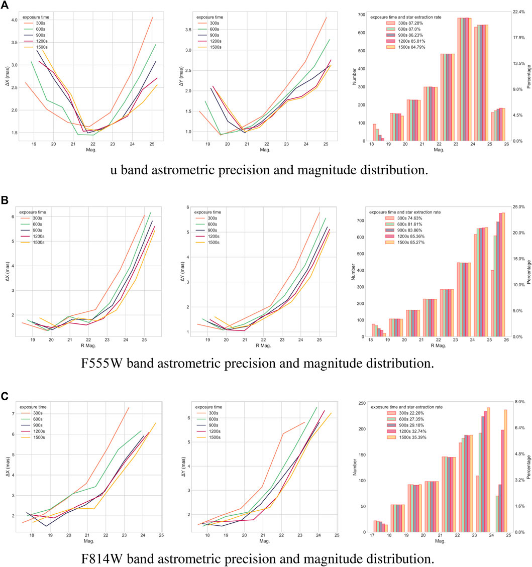
FIGURE 2. Astrometric precision with magnitudes and distribution of magnitudes for in I, R and G bands simulated images. Each subplot contains results under different exposure times. (A) The left and middle panels show the astrometric precision with magnitudes in pixel coordinates in u band image, and the right panel shows distribution of magnitudes and extracted rate of stars. (B) and (C) correspond to the F555W and F814W bands, respectively.

3 Simulated observations of M31

3.1 Velocity field model

The M31’s apparent size in the sky is about 3°10′ by 1°, therefore the factors such as kinematics, position of field, and more need to be considered for high precision astrometry. We use the analytical velocity field model presented by van der Marel et al. (2002) to describe PM field, because these equations are derived through mathematical deductions without other assumptions. For the planar system, the velocity of a tracer can be decomposed into the following three components 1:

$V=V_{\text{CM}}+V_{\text{pn}}+V_{\text{int}}(1)$

where V_CM is contributed by the space motion of center of M31, V_pn is contributed by precession and nutation, and it is small and is neglected, V_int is contributed by the internalrotation motion.

There are three coordinate systems as shown in Figure 3. The first Cartesian coordinate system (x, y, z): origin at the center of mass of M31, with the x-axis antiparallel to the right ascension axis, the y-axis parallel to the declination axis, and the z-axis toward the observer. The second Cartesian coordinate system (x′, y′, z′): origin at the center of mass of M31, with the (x′, y′)-plane is inclined with respect to the (x, y)-plane by the inclination angle i, the x′-axis along the intersection of the M31 disk plane and (x, y)-plane with position angle θ between the x-axis. The third Left-handed Cartesian coordinate system (x_l, y_l, z_l): origin at the center of the FOV, with z_l-axis along the line of sight, x_l along the tangent to the great circle at the origin, and the great circle pass the center of the M31 to the origin.

FIGURE 3

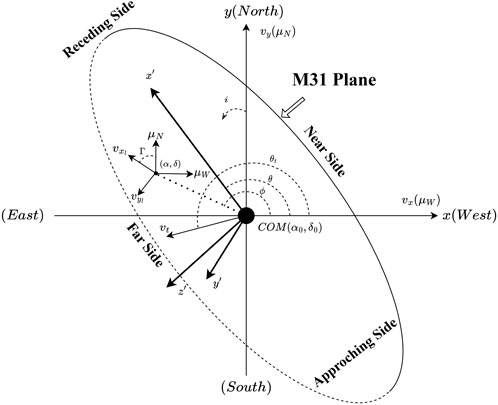
FIGURE 3. Illustration of coordinate systems and velocities for M31.

The Eq. 1 can be parameterized as follows in (2) and (3):

$\begin{array}{c}{V}_{\text{CM}}={\left(\begin{array}{c}\hfill v_{z_{\text{l}}}\hfill \\ \hfill v_{x_{\text{l}}}\hfill \\ \hfill v_{y_{\text{l}}}\hfill \end{array}\right)}_{\text{CM}}=\left(\begin{array}{c}\hfill v_t\sin \rho \cos \left(\varphi -{\theta }_t\right)+v_{\text{sys}}\cos \rho \hfill \\ \hfill v_t\cos \rho \cos \left(\varphi -{\theta }_t\right)-v_{\text{sys}}\sin \rho \hfill \\ \hfill -v_t\sin \left(\varphi -{\theta }_t\right)\hfill \end{array}\right)\hfill \\ V_{\mathrm{int}}={\left(\begin{array}{c}\hfill v_{z_{\text{l}}}\hfill \\ \hfill v_{x_{\text{l}}}\hfill \\ \hfill v_{y_{\text{l}}}\hfill \end{array}\right)}_{\text{int}}\hfill \\ =\frac{sV\left(R^{\prime }\right)}{{\left[{\cos }^{2}i{\cos }^2\left(\varphi -\theta \right)+{\sin }^2\left(\varphi -\theta \right)\right]}^{1/2}}\hfill \\ \times \left(\begin{array}{c}\hfill -\sin i\cos \left(\varphi -\theta \right)\left[\cos i\cos \rho -\sin i\sin \rho \sin \left(\varphi -\theta \right)\right]\hfill \\ \hfill \sin i\cos \left(\varphi -\theta \right)\left[\cos i\sin \rho +\sin i\cos \rho \sin \left(\varphi -\theta \right)\right]\hfill \\ \hfill -\left[{\cos }^{2}i{\cos }^2\left(\varphi -\theta \right)+{\sin }^2\left(\varphi -\theta \right)\right]\hfill \end{array}\right)\hfill \end{array}(2)$

$\begin{array}{ll}\hfill \left(\begin{array}{c}\hfill {\mu }_W\hfill \\ \hfill {\mu }_N\hfill \end{array}\right)& =\frac{\cos i\cos \rho -\sin i\sin \rho \sin \left(\varphi -\theta \right)}{D_0\cos i}\hfill \\ \hfill & \times \left.\left(\begin{array}{cc}\hfill -\sin \mathrm{\Gamma }\hfill & \hfill -\cos \mathrm{\Gamma }\hfill \\ \hfill \cos \mathrm{\Gamma }\hfill & \hfill -\sin \mathrm{\Gamma }\hfill \end{array}\right.\right)\left(\begin{array}{c}\hfill v_{x_{\text{l}}}\hfill \\ \hfill v_{y_{\text{l}}}\hfill \end{array}\right)\hfill \end{array}(3)$

These parameters in these equations are divided into four groups. The first group is the position of the field with respect to the center of M31: ρ is angular distance, ϕ is position angle. The second group describes the direction from which the plane of M31 is viewed: i is the inclination angle, θ is the position angle of the line of nodes. The third group describes the motion information of the center of M31: v_sys is the velocity along the line of sight, v_t and θ_t constitute the transverse velocity vector, D₀ is the distance to observer. The fourth group describes internal rotation: V(R′) is rotation velocity and s = ±1 determines the direction of rotation. Other quatities: ${\mu }_W=-{\mu }_{\alpha }^{*}$, μ_N = μ_δ, Γ is position angle of $v_{x_{\text{l}}}$ relative to the direction of positive declination.

For the simulated data, the above parameters can be categorized into two types, the first type is fixed value as follows: (i, θ) is (73.7°,128.3°), D₀ is 785 kpc, v_sys is 301 km/s (Karachentsev et al., 2004; McConnachie et al., 2005; Chemin et al., 2009). The second type will be fitted, but with initial values given to generate the simulated data, as follows: v_t is 160 km/s, θ_t is −2 rad and V(R′) is −230 km/s.

3.2 Local position distribution and motion

The stellar distribution of the disk of M31 is assumed to fit a classical surface density profile of the galactic disk, i.e., (Yin et al., 2009; Courteau et al., 2011), it can be represented by an exponential Eq. 4:

$M_r=M_0{e}^{-r/r_d}(4)$

where M₀ is the stellar density at the galactic center; r is the distance from the galactic center; r_d is the disk scalelength; M_r is the stellar density at the position with r distance from the galactic center. Given the simulation purpose, a typical scalelength, 5.5 kpc (Yin et al., 2009), is chosen to approximate the distribution of M31 member stars.

We assume that the spiral galaxy’s disk has an axisymmetric potential, and rotation curve is a function of disk stars’ circular velocity and distance from the disk center. The M31 rotation curve is obtained from Chemin et al. (2009) to approximate the circular motion of the M31 disk stars.

3.3 Simulated observed sky fields

Eight simulated observed fields, numbered from 1 to 8, are shown in Figure 4. Their celestial coordinates are (00h49m08.6s, 42°45′01.6″), (00h44m54.9s 40°57′13.1″), (00h36m37.4s 39°45′58.7″), (00h40m23.8s 41°36′06.3″), (00h48m15.4s, 41°51′54.0″), (00h41m19.4s 40°11′42.0″), (00h36m44.4s 40°26′06.0″), (00h45m00.0s 42°28′48.0″), respectively. The reason for these fields: (1) the field 1, the HST-observed field, can be compared. (2) they are located at approximately the same physical distance from the center of M31 disk, ensuring consistency in the rotational speed.

FIGURE 4

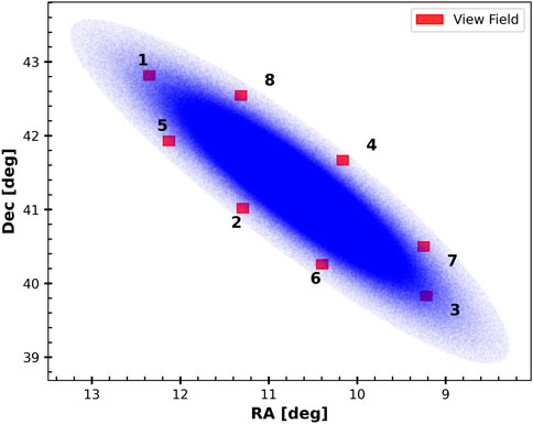
FIGURE 4. The simulated observed sky fields (red rectangles) in the M31.

4 Methods

This section presents methods for calculating the PMs of M31 member stars and Gaia DR3 reference stars. The parallax is neglected for M31 member stars for the large distance (785 ± 25 kpc). Finally, the PM results for the eight simulated fields are fitted to the motion of M31’s center by the velocity field model in sub Section 3.1.

4.1 Modification of Gaia DR3 reference stars’ PMs

The Gaia DR3 reference stars are selected for two reasons: First, they are point sources that offer higher astrometric precision, whereas extended sources such as background galaxies are limited by various shapes and sizes. Second, there are a large number of them, unlike the sparsely distributed quasars. There are 1288 QSOs in the 2° region centered on M31 (Liao et al., 2019), and the number in the simulated observed field is 1 or 2 and is approximately 1/100 of the Gaia reference stars. The advantage in terms of number (N) leads to an improvement in astrometric precision proportional to $\sqrt{N}$. When using Gaia catalog as the reference stars, the positional errors from the catalog are almost the same for M31 member stars at any epoch, so the errors do not dominate the error budget of PM result of M31 member stars. However, the PM errors from the catalog are cumulative for M31 member stars and are retained. Therefore, the PM errors have a significant impact on the precision of M31 PMs. It is necessary to modify the PMs of the catalog using observational images and then calculate the plate model parameters. At an observed epoch t, the pixel coordinates x(t), y(t) of reference stars are generated from the positions, positional errors, PMs, PM errors, parallaxes of the Gaia DR3 catalog, telescope parameters, etc. The celestial coordinates α_C(t), δ_C(t) of reference stars are extrapolated using the positions, PMs and parallaxes from the Gaia DR3 catalog, where the subscript “C” stands for catalog. The standard coordinates ξ_C(t), η_C(t) are obtained by performing a gnomonic projection equation of α_C(t), δ_C(t), as defined in Eq. 5.

$\begin{array}{cc}\hfill \xi & =\frac{\cos \delta \sin \left(\alpha -{\alpha }_0\right)}{\sin {\delta }_0\sin \delta +\cos {\delta }_0\cos \delta \cos \left(\alpha -{\alpha }_0\right)}\hfill \\ \hfill \eta & =\frac{\cos {\delta }_0\sin \delta -\sin {\delta }_0\cos \delta \cos \left(\alpha -{\alpha }_0\right)}{\sin {\delta }_0\sin \delta +\cos {\delta }_0\cos \delta \cos \left(\alpha -{\alpha }_0\right)}\hfill \end{array}(5)$

where α, δ denotes celestial spherical coordinates, with the subscript ’0’ (α₀, δ₀) meaning the celestial position of the plate center or “tangent-point” of the Cartesian coordinates, in which the η-axis is parallel to the declination axis and the ξ-axis is parallel to right ascension axis.

Then the plate model can be calculated by Eq. 6

$\begin{array}{c}\hfill {\xi }_{\text{C}}\left(t\right)=ax\left(t\right)+by\left(t\right)+c\\ \hfill {\eta }_{\text{C}}\left(t\right)=dx\left(t\right)+ey\left(t\right)+f\end{array}(6)$

where a, b, c, d, e, f is the affine transformation parameters between standard coordinates (ξ, η) and pixel coordinates (x, y), also known as the plate model. This plate model can be applied to the x(t), y(t) to obtain α_O(t), δ_O(t), where subscript “O” stands for observation. And, besides the simulated epochs, J2030.0 to J2039.0, the J2016.0 epoch from the Gaia DR3 catalog can be an additional observed epoch for modifying the PMs of the catalog. The PMs and errors, ${\mu }_{{\alpha *}_{\text{O}}},{\mu }_{{\delta }_{\text{O}}},\mathrm{\Delta }{\mu }_{{\alpha *}_{\text{O}}},\mathrm{\Delta }{\mu }_{{\delta }_{\text{O}}}$, are obtained by solving Eq. 7 (Perryman et al., 1997) using the least squares method.

$\begin{array}{c}{\xi }_{\text{O}}\left(t\right)=\frac{{\mu }_{{\alpha *}_{\text{O}}}\left(t-t_{\mathrm{r}\mathrm{e}\mathrm{f}}\right)-{\mathbf{p}}_{\mathrm{r}\mathrm{e}\mathrm{f}}{\mathbf{b}}_{\text{O}}\left(t\right)\pi /A}{1-{\mathbf{r}}_{\mathrm{r}\mathrm{e}\mathrm{f}}{\mathbf{b}}_{\text{O}}\left(t\right)\pi /A}+\mathrm{\Delta }\alpha *\hfill \\ {\eta }_{\text{O}}\left(t\right)=\frac{{\mu }_{{\delta }_{\text{O}}}\left(t-t_{\mathrm{r}\mathrm{e}\mathrm{f}}\right)-{\mathbf{q}}_{\mathrm{r}\mathrm{e}\mathrm{f}}{\mathbf{b}}_{\text{O}}\left(t\right)\pi /A}{1-{\mathbf{r}}_{\mathrm{r}\mathrm{e}\mathrm{f}}{\mathbf{b}}_{\text{O}}\left(t\right)\pi /A}+\mathrm{\Delta }\delta \hfill \\ {\mathbf{r}}_{\mathrm{r}\mathrm{e}\mathrm{f}}=\left(\begin{array}{c}\hfill \cos {\delta }_{\mathrm{r}\mathrm{e}\mathrm{f}}\cos {\alpha }_{\mathrm{r}\mathrm{e}\mathrm{f}}\hfill \\ \hfill \cos {\delta }_{\mathrm{r}\mathrm{e}\mathrm{f}}\sin {\alpha }_{\mathrm{r}\mathrm{e}\mathrm{f}}\hfill \\ \hfill \sin {\delta }_{\mathrm{r}\mathrm{e}\mathrm{f}}\hfill \end{array}\right){\mathbf{p}}_{\mathrm{r}\mathrm{e}\mathrm{f}}=\left(\begin{array}{c}\hfill -\sin {\alpha }_{\mathrm{r}\mathrm{e}\mathrm{f}}\hfill \\ \hfill \cos {\alpha }_{\mathrm{r}\mathrm{e}\mathrm{f}}\hfill \\ \hfill \mathbf{0}\hfill \end{array}\right)\hfill \\ {\mathbf{q}}_{\mathrm{r}\mathrm{e}\mathrm{f}}=\left(\begin{array}{c}\hfill -\sin {\delta }_{\mathrm{r}\mathrm{e}\mathrm{f}}\cos {\alpha }_{\mathrm{r}\mathrm{e}\mathrm{f}}\hfill \\ \hfill -\sin {\delta }_{\mathrm{r}\mathrm{e}\mathrm{f}}\sin {\alpha }_{\mathrm{r}\mathrm{e}\mathrm{f}}\hfill \\ \hfill \cos {\delta }_{\mathrm{r}\mathrm{e}\mathrm{f}}\hfill \end{array}\right)\hfill \end{array}(7)$

where subscript “ref” and “O” stands for reference and observation respectively; t_ref is the reference epoch; ${\mathbf{b}}_{\text{O}}\left(t\right)$ is the barycentric position of observer; π is parallax; A is astronomical unit; r_ref, p_ref and q_ref are orthogonal unit vectors, with original point (α_ref, δ_ref); Δα* = Δα cos δ_ref and Δδ are the residuals at the reference epoch in α_ref and δ_ref.

4.2 Calculation of M31 member stars’ PMs

Stationary reference sources, such as QSOs and background galaxies, can be used to align images from different observed epochs. To transform moving Gaia DR3 reference stars into “stationary”, we adopt the approach as shown in Figure 5: Select an epoch as reference epoch and the corresponding image as the reference image. Here, the intermediate epoch (J2035.0) is reference epoch, and represented by “mid”. The pixel coordinates of Gaia stars at other epochs can be adjusted to the intermediate epoch by applying the modified PMs Eq. 8.

$\begin{array}{c}\hfill x{\left(t\right)}_{\mathrm{m}\mathrm{i}\mathrm{d}}=x\left(t\right)+\left(t_{\mathrm{m}\mathrm{i}\mathrm{d}}-t\right)v_x\\ \hfill y{\left(t\right)}_{\mathrm{m}\mathrm{i}\mathrm{d}}=y\left(t\right)+\left(t_{\mathrm{m}\mathrm{i}\mathrm{d}}-t\right)v_y\end{array}(8)$

where t_mid is intermediate epoch; v_x, v_y are stellar velocities in the pixel coordinates; x(t)_mid, y(t)_mid are adjusted pixel coordinates. This adjustment ensures that each image at different epochs can be aligned with the reference image throught “stationary” Gaia stars, and the transformation as shown in Eq. 9.

$\begin{array}{c}\hfill x\left(t_{\mathrm{m}\mathrm{i}\mathrm{d}}\right)=ax{\left(t\right)}_{\mathrm{m}\mathrm{i}\mathrm{d}}+by{\left(t\right)}_{\mathrm{m}\mathrm{i}\mathrm{d}}+c\\ \hfill y\left(t_{\mathrm{m}\mathrm{i}\mathrm{d}}\right)=dx{\left(t\right)}_{\mathrm{m}\mathrm{i}\mathrm{d}}+ey{\left(t\right)}_{\mathrm{m}\mathrm{i}\mathrm{d}}+f\end{array}(9)$

where a, b, c, d, e, f are transformation parameters between images of one epoch and intermediate epoch. For M31 member stars in each image, applying affine transformation and the plate model at the intermediate epoch will convert pixel coordinates to celestial coordinates. Subsequently, the PMs of the M31 member stars can be calculated.

FIGURE 5

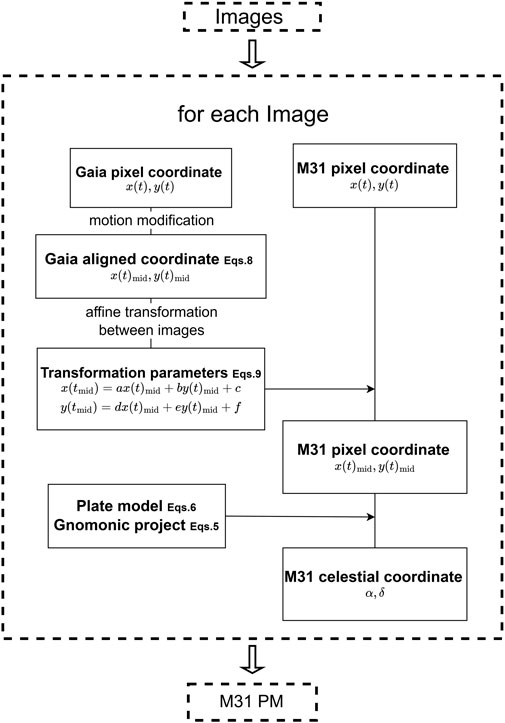
FIGURE 5. Flow chat for calculating PMs of M31 member stars.

5 Results

5.1 Theoretical PMs of M31 member stars

The adopted theoretical PMs of member stars within the first simulated observed field are calculated from J2030.0 to J2039.0, as shown in Figure 6. We assume that all member stars in the field have the same PM is unreasonable due to the significant degree of dispersion (∼3.0 μas/yr) relative to the expected observed PMs’ precision (∼10.0 μas/yr), and the field is divided into 2 × 2 blocks for reducing the degree. The distribution of one of the blocks is shown in Figure 7, where the dispersion of member stars is reduced to 1.5 μas/yr.

FIGURE 6

FIGURE 6. Histogram of adopted theoretical PMs in the first field. (A) RA PMs, (B) Dec. PMs.

FIGURE 7

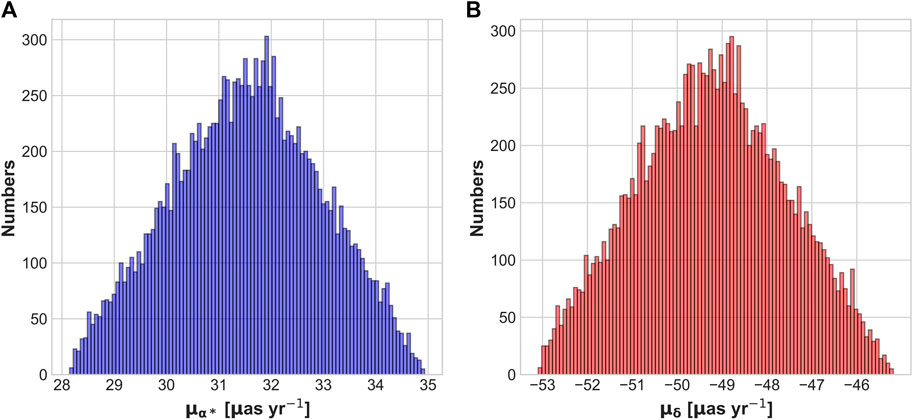
FIGURE 7. Histogram of adopted theoretical PMs of one block in the first field. (A) RA PMs, (B) Dec. PMs.

5.2 Simulated PMs of M31 member stars

The hypothetical strategy is to observe the all 8 fields quasi-simultaneously from J2030.0 to J2039.0, and the number of observed epochs per year is 1, 5, 10, 20 and 50. Figure 8 shows the relationship between the uncertainties of the average PMs within the first field and the number of observed epochs per year. It can be seen that uncertainty of 10 μas/yr is achievable with 10 epochs per year, and of 5 μas/yr with 50 epochs.

FIGURE 8

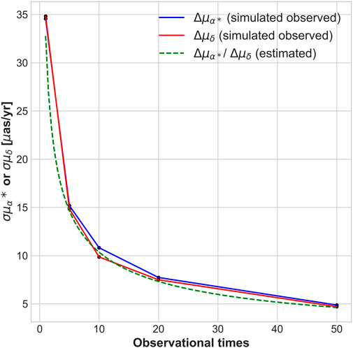
FIGURE 8. The relationship between the uncertainties of the average PMs within the first field and the number of observed epochs per year, positional uncertainties for reference stars and member stars are 0.05 pixels (2.5 mas) and 0.15 pixels (7.5 mas). The blue and red lines correspond to RA PMs and Dec. PMs, respectively. The green dashed line represents the PMs uncertainty estimated by the Eq. 10.

The uncertainty decreases with the increase in the number of epochs per year. But the improvement effect also keeps decreasing, 5 to 10 epochs achieves a good level of precision. There is simple Eq. 10 to estimate the uncertainty, which predicts only the Poisson noise’s behaviour and ignores the unknown systematic errors.

$\delta \approx \sqrt{{\sigma }_{\mathrm{r}\mathrm{e}\mathrm{f}}^2/N_{\mathrm{r}\mathrm{e}\mathrm{f}}+{\sigma }_{\text{member}}^2/N_{\text{member}}}/\sqrt{N_{\text{epoch}}}*\sqrt{2}/T_{\text{span}}(10)$

where σ_ref, σ_member are positional uncertainties for reference stars and M31 member stars; N_ref, N_member are corresponding star numbers; N_epoch is number of epochs per year; T_span is time span of PM calculation and $\sqrt{2}$ means displacement. Corresponding to 10 observed epochs in Figure 8, the values as follows: σ_ref, σ_member are 2.5 mas, 7.5 mas; N_ref, N_member are 165, ≈ 15000; N_epoch is 10; T_span is 9. And the result is 10.1 mas.

Using the simulated data provided above, the simulated PMs under 10 observed epochs per year are compared with the adopted theoretical values, as shown in Table 2. The differences between adopted theoretical and simulated observed values are introduced by PM errors in Gaia catalog.

TABLE 2

TABLE 2. Statistics of Theoretical and Simulated PM in The First Sky Field of Figure 4 Under 10 observed epochs per year.

5.3 Fitting motion of M31’s center and internal rotation

From Eqs 2, 3 in the velocity field model, the simulated observed PM results (μ_W, μ_N) or $({\mu }_{\alpha }^{*},{\mu }_{\delta })$ can be used to fit the information about M31’s kinematics. The parameters (i, θ, D₀, v_sys) are known, and parameters (ρ, ϕ) can be calculated based on the celestial coordinates of the field and M31’s center. The motion of M31’s center (v_t, θ_t), and internal rotational velocity (V(R′)) are obtained through the least-squares fit of PM results, as shown in Table 3.

TABLE 3

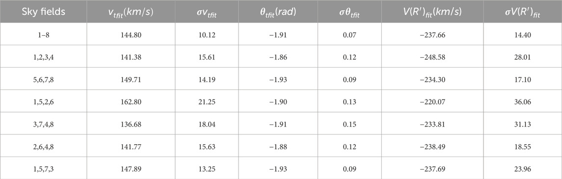
TABLE 3. Statistics of theoretical and fitted parameters of M31’s kinematics.

Analyzing the differences between adopted theoretical values v_t, θ_t, V(R′) (160 km/s, −2 rad, −230 km/s) and all fitting values, it could be found that these systematic errors are introduced by the PM errors in the Gaia catalog. Analyzing the differences in precision among fitted values from different fields, it could be found that with an increasing number of fields (1 to 8 fields), the precision improves. Under the condition of the same number of fields, if the fields are distributed on the same side (1, 5, 2, 6 fields or 3, 7, 4, 8 fields), the results are inferior to the symmetrically distributed fields. Under the condition where the observed fields are all symmetrically distributed, the fields away from the two sides of M31 (1, 3 fields) show better results in the internal rotation V(R′), and this may be the internal rotational motion contributes to the line-of-sight velocity at both ends. Furthermore, results of 5, 6, 7, 8 fields and 2, 6, 4, 8 fields show that having fields more dispersed might yield better results.

6 Conclusion

MCI, one of the backend modules of CSST, supports simultaneous UV-visible three-channel imaging. Its long focal length, high resolution, and deep detection depth make it suitable for high-precision space-based astronomical observations. In this paper, the astrometric capability of MCI is evaluated by using simulated observational images in the u, F555W and F814W bands, and then it is applied to calculate the simulated PMs of M31. MCI’s astrometric capability is reflected by the relationship between the positional uncertainty and magnitude, and it is influenced by the optical efficiency and filters’ bandwidth. Choosing R band as a reference for stellar positional precision, in which the bright-end stars (19–22 mag) are better than 2.0 mas, and the faint-end stars (22–25 mag) are better than 6.0 mas. Then, positional uncertainty of 2.5 mas for the brighter Gaia DR3 reference stars and of 7.5 mas for the fainter M31 member stars are adopted respectively. The simulation of M31’s motion using the velocity model is rough, but it is sufficient for the purpose of evaluating MCI’s astrometric capability and its application in measuring the motions of nearby external sources. The analysis of the simulated PMs of M31 member stars shows that increasing the number of observed epochs per year improves the precision of the PMs, and uncertainty of 10 μas/yr is achievable with 10 epochs per year, and of 5 μas/yr with 50 epochs. Considering the observational resources, achieving good precision with approximately 5–10 epochs per year is feasible, but this needs to be aligned with the actual observation plan. Additionally, selecting a larger number of observation fields that are symmetrically distributed and far from the approaching or receding side (as shown in Figure 3) of M31 will improve the precision of fitting the motion of M31. This may provide a reference for actual spatial observations of MCI.

It is noted that the simulated observational images used have not taken into account factors such as unknown systematic errors, field distortions, and cosmic ray effects, which may result in an overestimation of the precision of the PMs. In actual calculations of PMs, other factors need to be considered, such as damage of radiation for total ionizing dose (TID) and displacement damage effects, which degrade CCDs by decreasing the charge transfer efficiency (CTE) and increasing the mean dark current and hot pixels. Weighing the pros and cons of dithering, the pros: removal of cosmic rays, hot pixels, charge traps, improving spatial sampling; the cons: spacecraft overhead time, read noise, complicated data analysis, unsuitable for high-precision time-dependent photometry, and very short exposures. The observation schedule for M31, whether it is observable throughout all year and the distribution is uniform. Magnitude-dependent and color-dependent systematic errors between observations with different filters. Besides, to improve the precision of the PMs for M31, the previous HST observational data from 2002 could be combined with MCI to extend observed epochs. The above issues need to be further analyzed and validated in subsequent work.

Data availability statement

The raw data supporting the conclusion of this article will be made available by the authors, without undue reservation.

Author contributions

YY and XP proposed the method for calculating PMs. YY and WF analyzed MCI’s astrometric capability. WF simulated the motion of M31 member stars and calculated PMs with corresponding precision. ZY and HS provided the MCI simulated observational images and YH provided the star catalog used for generating these images. ZQ proposed the initial idea. SL and ZT provided suggestions on the method and structure of the paper. QW and ZF participated in the discussions. All authors contributed to the article and approved the submitted version.

Funding

This work has been supported by the National Natural Science Foundation of China (Grants No. 12073062 and 12173069), the Preresearch Project on Civil Aerospace Technologies funded by the China National Space Administration (Grant No. D010105). We also acknowledge the science research grants from the China Manned Space Project with Nos CMS-CSST-2021-A12, CMS-CSST-2021-B10, and CMS-CSST-2021-B04.

Acknowledgments

We use the CSST MCI image simulator to generate the mock data (https://csst-tb.bao.ac.cn/code/shaosim/mci). Gaia DR3 catalog from the European Space Agency (ESA) mission Gaia (https://www.cosmos.esa.int/gaia), processed by the Gaia Data Processing and Analysis Consortium (DPAC, https://www.cosmos.esa.int/web/gaia/dpac/consortium), has been utilized in this work.

Conflict of interest

The authors declare that the research was conducted in the absence of any commercial or financial relationships that could be construed as a potential conflict of interest.

Publisher’s note

All claims expressed in this article are solely those of the authors and do not necessarily represent those of their affiliated organizations, or those of the publisher, the editors and the reviewers. Any product that may be evaluated in this article, or claim that may be made by its manufacturer, is not guaranteed or endorsed by the publisher.

References

Bertin, E., and Arnouts, S. (1996). Sextractor: software for source extraction. Astronomy Astrophysics Suppl. 117, 393–404. doi:10.1051/aas:1996164

CrossRef Full Text | Google Scholar

Brown, A. G., Vallenari, A., Prusti, T., De Bruijne, J., Babusiaux, C., Biermann, M., et al. (2021). Gaia early data release 3-summary of the contents and survey properties. Astronomy Astrophysics 649, A1. doi:10.1051/0004-6361/202039657

CrossRef Full Text | Google Scholar

Chemin, L., Carignan, C., and Foster, T. (2009). H I kinematics and dynamics of messier 31. Astrophysical J. 705, 1395–1415. doi:10.1088/0004-637x/705/2/1395

CrossRef Full Text | Google Scholar

Chen, Y., Fu, X., Liu, C., Dal Tio, P., Girardi, L., Pastorelli, G., et al. (2023). The first comprehensive Milky Way stellar mock catalogue for the Chinese space station telescope survey camera. Sci. China Phys. Mech. Astronomy 66, 119511. doi:10.1007/s11433-023-2181-x

CrossRef Full Text | Google Scholar

Courteau, S., Widrow, L. M., Mcdonald, M. A., Guhathakurta, P., Majewski, S. R., Zhu, Y., et al. (2011). The luminosity profile and structural parameters of the andromeda galaxy. Astrophysical J. 739, 20–954. doi:10.1088/0004-637x/739/1/20

CrossRef Full Text | Google Scholar

Karachentsev, I. D., Karachentseva, V. E., Huchtmeier, W. K., and Makarov, D. I. (2004). A catalog of neighboring galaxies. Astronomical J. 127, 2031–2068. doi:10.1086/382905

CrossRef Full Text | Google Scholar

Liao, S.-L., Qi, Z.-X., Guo, S.-F., and Cao, Z.-H. (2019). A compilation of known QSOs for the Gaia mission. Res. Astronomy Astrophysics 19, 029. doi:10.1088/1674-4527/19/2/29

CrossRef Full Text | Google Scholar

Lindegren, L., Klioner, S., Hernández, J., Bombrun, A., Ramos-Lerate, M., Steidelmüller, H., et al. (2021). GaiaEarly Data Release 3: parallax bias versus magnitude, colour, and position. Astronomy Astrophysics 649, A4. doi:10.1051/0004-6361/202039653

CrossRef Full Text | Google Scholar

McConnachie, A. W., Irwin, M. J., Ferguson, A. M., Ibata, R., Lewis, G., and Tanvir, N. (2005). Distances and metallicities for 17 local group galaxies. Mon. Notices R. Astronomical Soc. 356, 979–997. doi:10.1111/j.1365-2966.2004.08514.x

CrossRef Full Text | Google Scholar

Perryman, M., O’Flaherty, K. S., and van Leeuwen, F. (1997). The hipparcos and tycho catalogues: astrometric and photometric star catalogues derived from the ESA. Noordwijk, Netherlands: ESA Publications Division.

Google Scholar

Salomon, J., Ibata, R., Reylé, C., Famaey, B., Libeskind, N., McConnachie, A., et al. (2021). The proper motion of Andromeda from Gaia EDR3: confirming a nearly radial orbit. Mon. Notices R. Astronomical Soc. 507, 2592–2601. doi:10.1093/mnras/stab2253

CrossRef Full Text | Google Scholar

Sohn, S. T., Anderson, J., and Van der Marel, R. P. (2012). The M31 velocity vector. I. Hubble Space Telescope proper-motion measurements. Astrophysical J. 753, 7. doi:10.1088/0004-637x/753/1/7

CrossRef Full Text | Google Scholar

Vallenari, A., Brown, A., Prusti, T., de Bruijne, J., Arenou, F., Babusiaux, C., et al. (2023). Gaia Data Release 3-summary of the content and survey properties. Astronomy Astrophysics 674, A1. doi:10.1051/0004-6361/202243940

CrossRef Full Text | Google Scholar

van der Marel, R. P., Alves, D. R., Hardy, E., and Suntzeff, N. B. (2002). New understanding of Large Magellanic Cloud structure, dynamics, and orbit from carbon star kinematics. Astronomical J. 124, 2639–2663. doi:10.1086/343775

CrossRef Full Text | Google Scholar

van der Marel, R. P., Fardal, M. A., Sohn, S. T., Patel, E., Besla, G., del Pino, A., et al. (2019). First Gaia dynamics of the Andromeda system: DR2 proper motions, orbits, and rotation of M31 and M33. Astrophysical J. 872, 24. doi:10.3847/1538-4357/ab001b

CrossRef Full Text | Google Scholar

Yan, Z.-J. (2023). The instrument simulating of Multi-Channel Imager on the CSST. In preparation.

Google Scholar

Yin, J., Hou, J., Prantzos, N., Boissier, S., Chang, R., Shen, S., et al. (2009). Milky Way versus Andromeda: a tale of two disks. Astronomy Astrophysics 505, 497–508. doi:10.1051/0004-6361/200912316

CrossRef Full Text | Google Scholar

Zhan, H. (2011). Consideration for a large-scale multi-color imaging and slitless spectroscopy survey on the Chinese space station and its application in dark energy research. Sci. Sinica Phys. Mech. Astronomica 41, 1441–1447. doi:10.1360/132011-961

CrossRef Full Text | Google Scholar

Zhan, H. (2021). The wide-field multiband imaging and slitless spectroscopy survey to be carried out by the Survey Space Telescope of China Manned Space Program. Chin. Sci. Bull. 66, 1290–1298. doi:10.1360/tb-2021-0016

CrossRef Full Text | Google Scholar