Forecasting solar flares with a transformer network

Space weather phenomena, including solar flares and coronal mass ejections, have significant influence on Earth. These events can cause satellite orbital decay due to heat-induced atmospheric expansion, disruption of GPS navigation and telecommunications systems, damage to satellites, and widespread power blackouts. The potential of flares and associated events to damage technology and disrupt human activities motivates prediction development. We use Transformer networks to predict whether an active region (AR) will release a flare of a specific class within the next 24 h. Two cases are considered: ≥C-class and ≥M-class. For each prediction case, separate models are developed. We train the Transformer to use time-series data to classify 24- or 48-h sequences of data. The sequences consist of 18 physical parameters that characterize an AR from the Space-weather HMI Active Region Patches data product. Flare event information is obtained from the Geostationary Operational Environmental Satellite flare catalog. Our model outperforms a prior study that similarly used only 24 h of data for the ≥C-class case and performs slightly worse for the ≥M-class case. When compared to studies that used a larger time window or additional data such as flare history, results are comparable. Using less data is conducive to platforms with limited storage, on which we plan to eventually deploy this algorithm.

1 Introduction

Solar flares are often defined as intense, localized bursts of electromagnetic radiation from the Sun occurring on the timescale of minutes to hours (Benz, 2017). Powerful flares can cause satellite orbital decay due to heat-induced atmospheric expansion (Schwenn, 2006). Moreover, such flares are often associated with solar energetic particle events (SEPs) and coronal mass ejections (CMEs) (Schwenn, 2006), which have the potential to induce further severe consequences. For example, SEPs, which may reach the Earth soon after the flare does, can harm astronauts, disrupt GPS navigation, and damage satellite systems (Pulkkinen, 2007). CMEs, which can take from hours to days to reach the Earth, may cause geomagnetically induced currents (Pulkkinen et al., 2003). These can corrode pipes, disrupt telecommunications devices, and permanently damage transformers, potentially leading to widespread and long-term power blackouts (Pulkkinen, 2007).

In light of such severe consequences, it has become the subject of much research to predict these events. However, the physical processes underlying solar flares are not well understood. It is suggested that the energy release is the result of magnetic reconnection, where accumulated energy in the magnetic field is impulsively released when the field falls to a lower-energy state (Benz, 2017). Flares tend to occur in locations at which the magnetic field is strongly sheared (Hagyard et al., 1984), where magnetic flux emerging from below the sheared field can destabilize the magnetic structures, causing impulsive energy release (Choudhary et al., 1998). Photospheric magnetic field shear and flux parameters are among those in the Space-weather HMI Active Region Patches (SHARPs) data product (Bobra et al., 2014), which is recorded by the Helioseismic and Magnetic Imager (HMI) aboard the Solar Dynamics Observatory (SDO) and consists of data collected since 2010. The SHARPs data series contains multiple physical parameters characterizing the photospheric vector magnetic field for automatically detected and tracked active regions (ARs) over the duration of their lifetimes at a cadence of 12 min (Bobra et al., 2014).

Various AI methods are used in heliophysics to tackle problems ranging from transportation of the charged particles throughout the heliosphere (Inceoglu et al., 2022a) to detecting magnetic activity structures on the Sun (Jarolim et al., 2021; Inceoglu et al., 2022b) and to predicting CMEs (Inceoglu et al., 2018; Raju and Das, 2023), as well as predicting the occurrences of solar flares with a forecast window of 24–48 h. In 2015, Bobra and Couvidat (2015) trained a support vector machine (SVM) algorithm on SHARPs data to classify whether an AR would emit a flare. In 2018, Nishizuka et al. (2018) used vector magnetograms, along with 1,600 and 131 Å filter images and soft X-ray emission light curves, to train a deep neural network to predict whether an AR would release a flare of a specific magnitude within 24 h. The authors later applied this algorithm to develop an operational solar flare prediction model (Nishizuka et al., 2021). Jonas et al. (2018) attempted a similar prediction task, but using image data recorded by the Atmospheric Imaging Assembly aboard the SDO satellite along with SHARPs data. The authors used 1,600, 171, and 193 Å images describing the photosphere, chromosphere, transition region, and corona. Florios et al. (2018) also used image data, but instead calculated predictors from SHARPs line-of-sight (LoS) magnetograms to train multilayer perceptron, SVM, and random forest algorithms. Liu et al. (2019) conducted one of the first studies fully utilizing the time dependence of the SHARPs datatset. The authors trained a long short-term memory (LSTM) network on various SHARPs photospheric magnetic field parameters and flare history parameters. A similar study was conducted by Wang et al. (2020), who only used photospheric vector magnetic field parameters from the SHARPs data series to train an LSTM. Similar to Florios et al. (2018), Li et al. (2020) used LoS SHARPs magnetograms, but instead trained a deep convolutional neural network (CNN). Ribeiro and Gradvohl (2021) used ensemble learning methods to combine the predictions of SVM, Random Forest, and Light Gradient Boosting Machine algorithms that had been trained on multiple datasets, including SHARPs. This study did not use the input data as a time series, but retained some temporal information by utilizing features calculated from the time leading up to the flare. Transformers are another recently developed type of neural network designed around self-attention mechanisms that enable the extraction of relevant data from a sequence (Bahdanau et al., 2014) without the need for recurrence (Vaswani et al., 2017). Thus far, only Abduallah et al. (2023) has applied this network to flare forecasting, developing an operational model using a Transformer + CNN + LSTM network.

In this study, we use Transformer networks to predict whether an AR will release a flare of a specific magnitude within 24 h after measurement. The rest of this paper is organized as follows. Section 2 describes the data features, preprocessing steps, Transformer model architecture, training process, and performance metrics. Section 3 describes threshold selection and analyzes experimental results. Section 4 compares our results with those from prior studies and discusses next steps and further applications.

2 Methods

2.1 Data and preprocessing

Our study utilizes the SHARPs data product, which consists of data recorded by the Helioseismic and Magnetic Imager aboard the Solar Dynamics Observatory (Bobra et al., 2014). The HMI instrument measures the photospheric magnetic field every 12 min for ARs that are tracked for their entire lifetimes (Bobra et al., 2014). From these measurements, various parameters are calculated that characterize the behavior of the magnetic field in each AR at each time step. The 18 parameters used in this study are described in Table 1, and are downloaded for ARs from May 2010 through December 2022. To ensure data quality, data are only downloaded if they meet the following conditions: 1) the absolute value of the orbital velocity of the SDO satellite is less than 3,500 m s⁻¹ and 2) data are of high quality (the signal-to-noise ratio is low and there are no problems with the observation, i.e., an eclipse).

TABLE 1

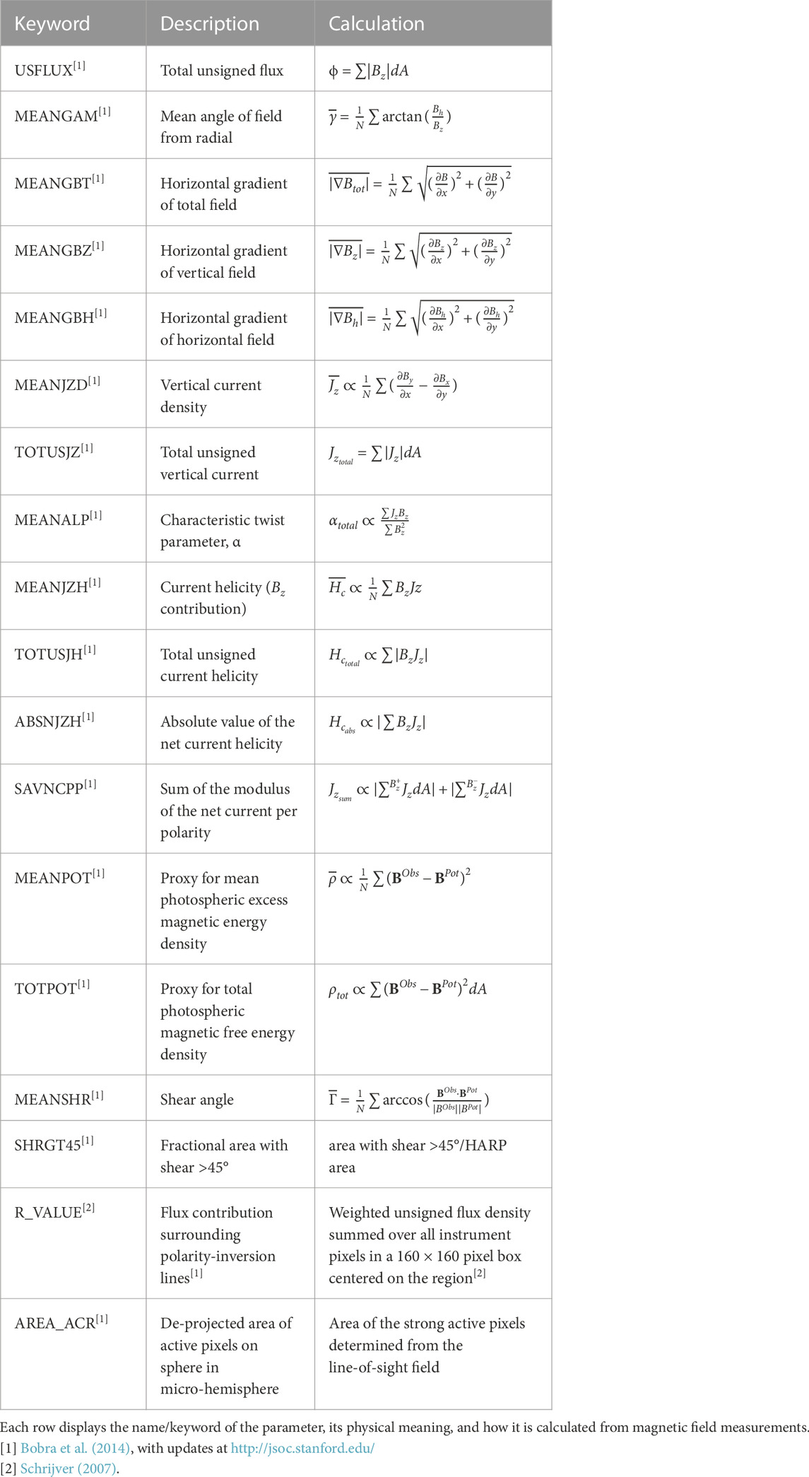
TABLE 1. Summary of the 18 physical SHARPs parameters used in this study.

Flare event data are obtained from X-ray flux measurements made by the Geostationary Operational Environmental Satellite (GOES) operated by the National Oceanic and Atmospheric Administration (NOAA). The GOES satellite detects solar flares through observation of X-rays, yielding a flare catalog providing information including event start/peak/end times, flare class, and NOAA active region number (Garcia, 1994). Flares are classified by the peak soft X-ray (SXR) flux observed by the GOES satellite, as seen in Table 2. The GOES data are then used to classify the SHARPs data by GOES flare class and to extract the measurements occurring before the peak time. SHARPs data for which no corresponding NOAA number can be found in the GOES catalog are ignored. The result is a time series of SHARPs parameter values leading up to each flare and separated by flare class. The number of ARs corresponding to each class are displayed in Table 2. It should be noted that there are very few A-class events only because their emission may not be intense enough to be detected over the X-ray background (Wang et al., 2020).

TABLE 2

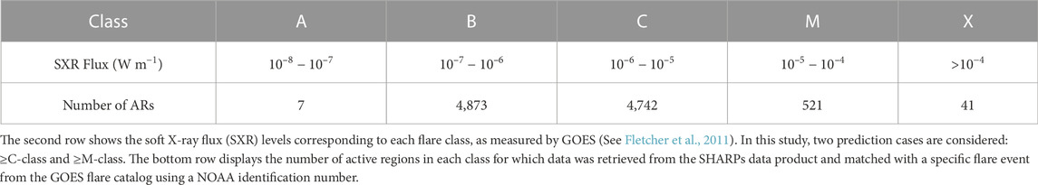
TABLE 2. Flare classification system and number of corresponding active regions used in this study.

Following the generation of SHARPs data leading up to each flare, which are sorted by flare class, several preprocessing steps are applied. Missing timesteps are filled through linear interpolation, and NaN values at the beginning or end of the time series are filled using backward/forward fill. This process avoids errors caused by one or more parameters not being present at any time step. Any sequences that contain less than 48 h of data are removed. The resulting sequences (time-series) are then converted to first-degree difference sequences, which consist of the changes from each data point to the next. This process is highly computationally efficient and does not compromise performance.

After the data preparation process, input data are generated. The following process generates the 24-h data window, but the general process remains the same for the 48-h case. First, for each sequence in each flare class, data recorded until at least 48 h before the flare peak are defined as pre-window and data recorded within 48 h of the flare peak are defined as intra-window. The resulting sequences are then divided into positive and negative groups, depending on the prediction case (≥C vs. ≥M). For instance, for the ≥C-class case, the negative set consists of all A-class, B-class, pre-window C-, M-, and X-class sequences while the positive set consists of intra-window C-, M-, and X-class sequences. This split is depicted in Figure 1. Note that this figure only depicts the ≥C-class prediction case, as the flare magnitude cutoff (negative vs. positive) would change for the ≥M-class case. Next, for each sequence (positive or negative), different 24-h long sequences starting at random times are generated. These are the sequences that are fed into the model. Generating random data sequences at different times enables within-24-h prediction, instead of selecting a fixed window. This data generation process (random 24/48-h sequence extraction) is done separately for each prediction case (flare class and data duration), so no two models have the same input data set.

FIGURE 1

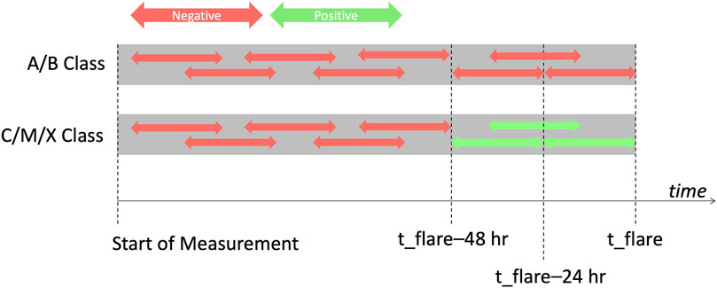
FIGURE 1. Data splitting methodology for the ≥C-class prediction case using 24 h of data. Each grey block represents a pre-flare sequence of SHARPs time-series data. If the corresponding flare is an A- or B-class flare (the top grey block), all generated sequences are classified as negative (as represented by red arrows, 24 h in length). For C-, M-, or X-class flares (the bottom row), sequences ending within 24 h of the flare peak time (t_flare) are labeled as positive (depicted as green arrows in the figure). Since the sequences are 24 h long, any sequences starting within 48 h of the flare peak (after t_flare−48 h) are labeled as positive. This results in any 24-h sequences in which a ≥C-class flare occurs within 24 h after measurement being classified as positive.

After generating model input data, we shuffle the data and randomly split it into training, validation, and testing data for the machine learning model. In this study, 20% of the data are used as testing data, while 80% are used as training data. Of the 80% that is allotted to training, 20% are used for validation. This is also done separately for each prediction case, yielding different data sets for each model. After train/test splitting, input data sets (train, test, validation) are normalized by scaling relative to the maximum values for the corresponding parameter found in the training data. In addition, we acknowledge that although methods such as k-fold cross-validation would provide more statistical robustness to the results, they are not feasible computationally. Even with 2 x RTX4090 GPUs with a total of 128 GB of memory, computation is limited because each of the training data sets is over 35 GB, and the hyperparameter search space is unconventionally large (see Section 2.2). Therefore, we do not include such methods.

Because 24-h sequences are generated at random times within each data window, some sequences may overlap. When sequences are then split randomly into training and testing data, some parts of sequences may appear in both the training and testing data. We acknowledge that this may cause slight artificial gain in performance of the model on the testing set. This could be addressed by separation of training/testing data by year. However, it has been shown that separating training/testing data by year yields significantly different results depending on the years selected (Wang et al., 2020), which may be due to the solar cycle. For instance, Wang et al. (2020) demonstrated that the True Skill Statistic (TSS) may change by more than 0.20 TSS units for the ≥M-class case, depending on which year is selected for testing.

Due to the rarity of severe flare events, the training data set is highly imbalanced, meaning that there are vastly fewer severe flares (≥M or ≥C, depending on the prediction case) than non-severe events. This is unsuitable for model training for flare prediction purposes. If a model is trained on a data set containing a vast majority of negative examples, it will simply learn to predict that all examples are negative. While this may achieve high accuracy, it does not have any predictive value. To overcome this issue, we undersample the negative class by randomly removing enough negative examples to yield a balanced training data set. The validation set remains imbalanced, enabling model parameters to still be optimized according to the imbalanced nature of flare prediction. The undersampling process is also done separately for each prediction case. Nishizuka et al. (2018), Liu et al. (2019), and Wang et al. (2020) all use various cost functions to address the imbalance (usually a form of cross-entropy) and do not use data balancing techniques. While we do use a similar cost function, we also use undersampling techniques, leading to more efficient computation and data storage.

2.2 Network architecture and training

The Transformer network utilizes self-attention mechanisms to process time series data without the need for recurrence (Vaswani et al., 2017). It was originally designed for sequence modeling and transduction, specifically natural language processing tasks such as translation and English constituency parsing. Since 2017, it has been applied successfully to video action detection (Girdhar et al., 2019), skin lesion analysis (He et al., 2022), anomaly detection (Tuli et al., 2022), protein prediction (Nambiar et al., 2023), earthquake location (Münchmeyer et al., 2021), and further diverse applications. The multivariate time series data of the photospheric magnetic field parameters may be suitable to the application of the Transformer. Self-attention mechanisms enable a model to extract the most important parts of a sequence (Bahdanau et al., 2014). They can learn interdependencies among variables to process sequences such as time series data for tasks such as classification or translation. By eliminating recurrence through the use of these mechanisms, Transformer models are more parallelizable, achieving state-of-the-art performance with significantly reduced processing times (Vaswani et al., 2017).

The architecture of our Transformer model is shown in Figure 2. The input sequence, which spans 24 h, is input into a Transformer encoder (orange block in Figure 2). The first residual connection splits off at this point. The input is then normalized and sent to the multi-head attention (MHA) block. This primarily consists of several scaled dot-product attention layers running simultaneously, enabling the model to ‘attend to’ different parts of the sequence (Vaswani et al., 2017) and to extract the parts that are more relevant to classification. The resulting vector is then sent to a dropout layer, which is used to prevent the neural network from overfitting by dropping a specific proportion of units randomly (Srivastava et al., 2014). The output of this layer is then added to the original input that previously split off as a residual connection. The purpose of this residual connection is to enable a channel of information flow that is unaffected by the attention mechanism, resulting in easier model optimization (He et al., 2016). Another residual connection splits off at this point, while the main information flow is normalized and sent to a feed-forward network. We use three layers of convolution kernels that are convolved with the normalized data in one dimension. Dropout layers are also added between Conv1D layers. The output of the feed forward part is then added to the residual connection that previously split off. The result is the output of the Transformer encoder. This output vector is then fed back into another Transformer encoder. This is repeated for N transformer encoder blocks (bottom right of Figure 2). The output vector of the Nth encoder block is sent to an average pooling layer that reduces its size and makes the model more robust to noise and small variations (Boureau et al., 2010). The output is then sent to a multi-layer perceptron (MLP). The purpose of the MLP is to process the output vector of the Transformer encoder for binary classification. Our MLP consists of 3 densely connected layers followed by a dropout layer. Finally, there is an output layer of size one with the sigmoid activation function, which converts the single probability value returned by the final neuron to a probability of belonging to the positive class with a range of (0,1). The final class label is later obtained by comparison to a chosen threshold; if the output lies above that threshold, it is classified as positive (otherwise it is classified as negative).

FIGURE 2

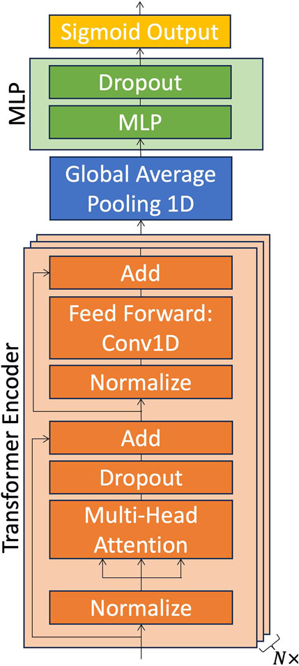
FIGURE 2. Our model architecture. The input sequence is first passed into N transformer encoder blocks (depicted in orange), which each include a multi-head attention block and a feed-forward block. Then, after a pooling layer (blue), there is a multi-layer perceptron (MLP) with dropout, depicted in green. The last yellow layer represents the final output neuron, which is activated by the sigmoid function.

The Transformer model is trained using the Adam optimizer (Kingma and Ba, 2015), with the learning rate as one of the hyperparameters to be optimized and all other parameters set to default. We use the Binary Cross-Entropy loss function (shown in Eq. 1) as the cost to be optimized. In this equation, N is the number of sequences and K is the number of classes. w_k represents the weight of class k (which gives more importance to positive examples). y_nk is the true class label, while ${\widehat{y}}_{nk}$ is the predicted probability of the sequence belonging to the positive class.

$J={\displaystyle \sum _{n=1}^N}{\displaystyle \sum _{k=1}^K}{w}_k{y}_{nk}\log \left({\widehat{y}}_{nk}\right)(1)$

During training, the model is evaluated on three scores: accuracy, area under the receiver operating characteristic curve (ROC_AUC), and area under the precision-recall curve (PR_AUC). Accuracy indicates the proportion of all samples that are classified correctly. The ROC curve plots the true positive rate (recall) vs. false positive rate for thresholds ranging from 0 to 1 (Marzban, 2004). When the area under the curve (AUC) is evaluated, it provides an overall measure of model performance across various classification thresholds, with larger ROC_AUC values indicating better performance. We use this metric because it does not require choosing a specific threshold (Marzban, 2004), enabling us to later select a threshold to optimize performance. The precision-recall curve plots precision and recall for the same threshold range (0–1) to show the trade-off between precision and recall, and the area under this curve indicates overall performance across thresholds. See Section 3.1 for further discussion of precision and recall. Another way of tackling this issue is to use a cost function, the so-called Score-Oriented Loss (SOL) function (Marchetti et al., 2022), which prioritizes a selected evaluation metric to optimize the DL (deep learning) model to maximize it.

Model hyperparameter optimization is achieved using Bayesian optimization, a method which enables selection of hyperparameters based on results of prior combinations (Wu et al., 2019). The hyperparameters, search spaces, and optimized values are shown in Table 3. The objective of the Bayesian optimization method is to maximize the ROC_AUC achieved on the validation set. The maximum number of trials, or hyperparameter combinations tested, is set to 10. The number of executions per trial is set to 1. These parameters are limited due to the lack of computational power available, as described previously. Limitations are exacerbated by our extended optimization process, which includes hyperparameters beyond those conventionally examined (See Table 3). The various model configurations are tested with 100 epochs, but are set to stop training when the ROC_AUC does not improve over 5 epochs. Once the best hyperparameters have been found through Bayesian optimization, the model is re-trained using the selected values and a batch size of 32, then saved. The methods described in this section are implemented in Python with Tensorflow and Keras.

TABLE 3

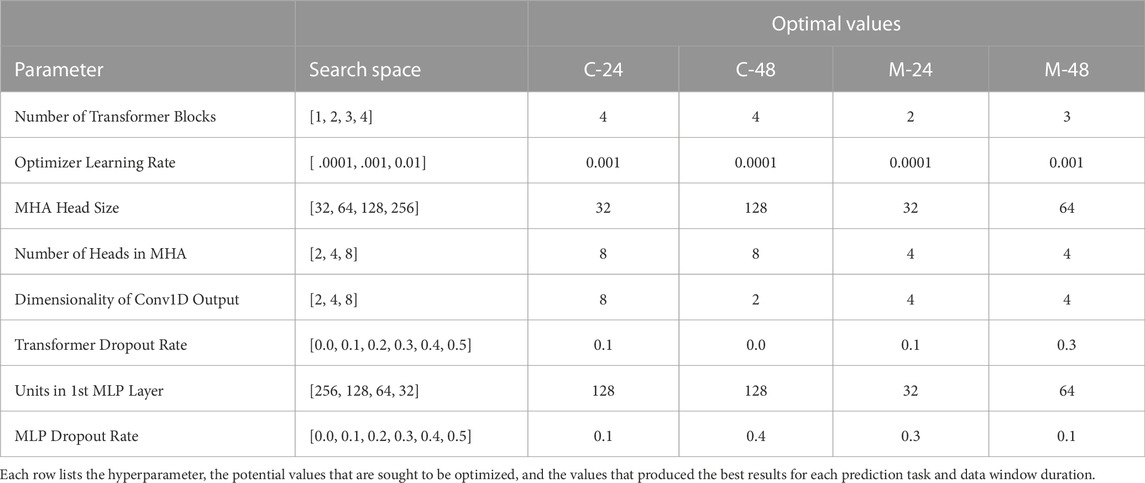
TABLE 3. Hyperparameter search space and optimal values.

2.3 Performance metrics

Once the model has been trained on the training/validation data sets, it is evaluated on the test set, which consists of previously unseen sequences. First, a threshold is chosen to obtain predicted class labels. Then, a confusion matrix is generated by calculating the number of correctly and incorrectly predicted examples in each class. Figure 3 illustrates a confusion matrix and lists values for each of the four prediction cases. When an example sequence is classified by the model, there are four possible outcomes relative to the correct label: 1) True Positive (TP): the model correctly classifies it as positive, 2) False Negative (FN): the model incorrectly classifies it as negative, 3) False Positive (FP): the model incorrectly classifies it as positive, and 4) True Negative (TN): the model correctly classifies it as negative. The confusion matrix shows the number of examples resulting in each of these outcomes. Any metrics not reported in this paper can be calculated from the values given in Figure 3.

FIGURE 3

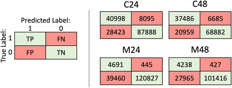
FIGURE 3. Confusion matrices. The matrix on the left depicts a generic confusion matrix, where each cell shows the number of examples corresponding to that outcome. TP is True Positive, FN is False Negative, FP is False Positive, and TN is True Negative. The results for each of the 4 models are shown on the right. These values are then used to calculate model evaluation metrics (see Section 3.1)

Once the four values are calculated (TP, FN, FP, TN), model performance can be assessed through the calculation of performance metrics. These metrics are described in Table 4. Accuracy (ACC) describes the total proportion of examples that the model correctly classifies. This metric should not be used in imbalanced classification tasks such as flare prediction because a model may reach high accuracy by learning to classify all examples as belonging to the majority class (He and Garcia, 2009). Despite achieving high accuracy, such a model would have no predictive value. Instead of accuracy, balanced accuracy (BACC) is used. This metric is equivalent to accuracy calculated with weighted values determined by the class imbalance, and is calculated by averaging the true positive rate (recall) and the true negative rate (Brodersen et al., 2010). The true positive rate (also known as recall) is the proportion of positive examples that the model correctly classifies. Likewise, the true negative rate is the proportion of negative examples correctly classified. In addition to ACC and BACC, we use precision (PRE) and recall (REC) to provide information concerning the ability of the model to correctly identify positive (severe) flares. Precision indicates the accuracy of positive predictions. This metric is useful in describing the reliability of severe flare predictions. Precision and recall are especially relevant in cases like flare prediction where it is important for any model deployed in an operational setting to not ‘miss’ any severe events but also to not have too many false alarms. To incorporate both of these ideas, Hanssen and Kuipers (1965) developed the True Skill Statistic (TSS). This is calculated by subtracting the false alarm rate from the recall value, balancing PRE and REC. While a model that is trained to frequently predict the positive case will have a high recall value, it will also often have many false alarms, thereby reducing precision. Such a model would produce a low TSS score, providing more useful information regarding the predictive value of the model. This metric is especially suitable to imbalanced prediction cases such as flare prediction because it is unaffected by the class imbalance (Woodcock, 1976). Lastly, the Heidke Skill Score (HSS) is used, a metric which describes how the model performs relative to a random chance prediction (Heidke, 1926). This provides useful information on the predictive value of the model and has the benefit of using all four confusion matrix values (Bloomfield et al., 2012), although it should be noted that TSS also uses all four values.

TABLE 4

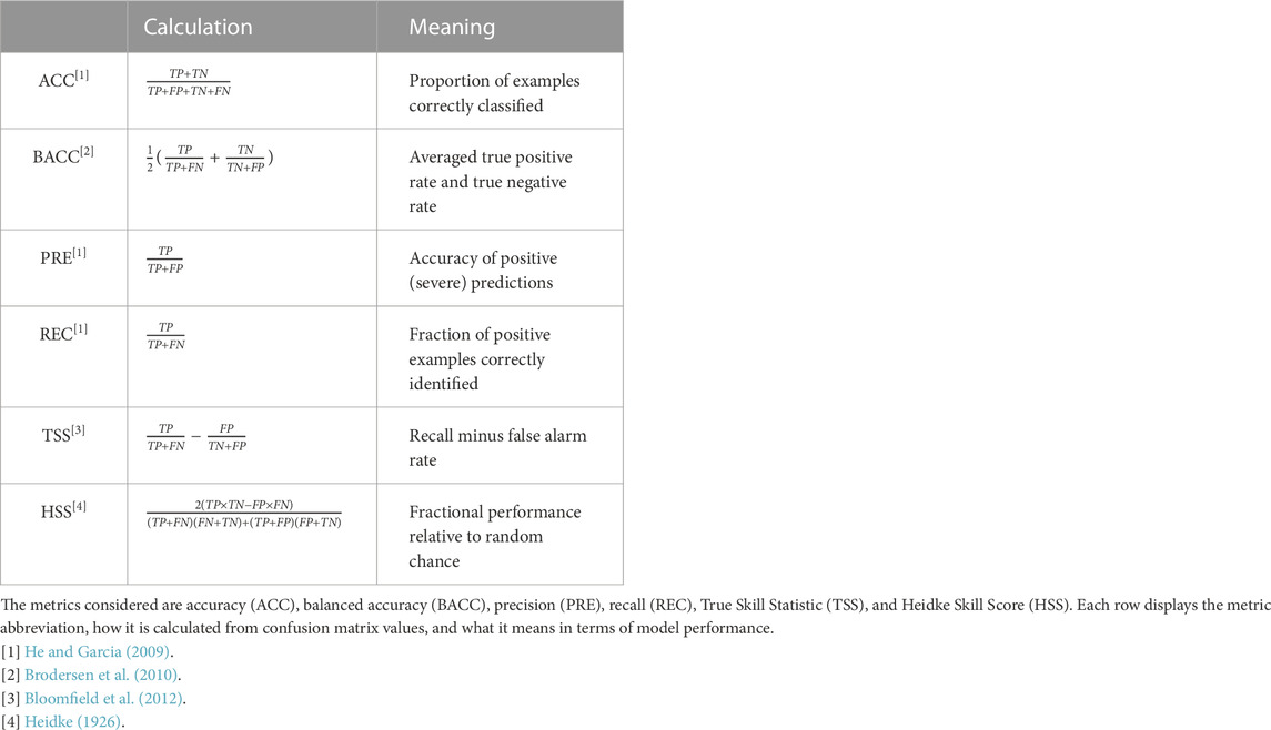
TABLE 4. Definitions of various model evaluation metrics.

3 Results

3.1 Performance metric scores

The output of the model for a single example is the probability of belonging to the positive class, which ranges from 0 to 1. In order to obtain a class label, it must be compared to a threshold (above which it is classified as positive). We select this threshold such that overall performance is maximized. We calculate each of the six metrics for all thresholds in the range 0.05–0.95. Figure 4 displays each metric as a function of threshold for all four models. The general shapes of the performance curves do not vary dramatically with different data window lengths (24 vs. 48 h). However, there is a significant difference between the curve shapes for the two class cases (≥M vs. ≥C). While the ≥C-class curves have an area where performance is clearly optimized, the ≥M-class curves are relatively flat on the left side of the graphs; the overall model performance for all thresholds less than ∼0.5 is very similar. This can be explained by the distribution of model output probabilities. For the 24-h data window case for ≥ M-class case, 82% of the model output probabilities lie either under 0.1 or over 0.6 (for the ≥C-class variation, this figure drops to 64%). This means that relatively few flares produce output probabilities between 0.1 and 0.6, resulting in flat skill score curves in the range.

FIGURE 4

FIGURE 4. Evaluation metrics across thresholds for all four prediction cases (≥C-class with a 24-h data window, ≥C-class with a 48-h data window, ≥M-class with a 24-h data window, and ≥M-class with a 48-h data window). Six metrics were calculated for test set predictions for all thresholds between 0.05 and 0.95, inclusive. The threshold chosen, which is shown with a vertical red line, is where the maximum TSS score occurs. Threshold values yielding maximum performance are shown in Table 6.

3.1.1 Accuracy and balanced accuracy

The maximum scores of each metric for each prediction case (flare class and data window) are displayed in Table 5. The table also displays the thresholds at which these maxima occur. Note that these scores are not our final model scores. For the ≥C-class case with 24 h of data, a maximum accuracy of 0.811 is reached with a threshold of 0.76. For the 48-h case, a score of 0.816 is reached with a threshold of 0.72. When considering the ≥M-class case, the 24-h and 48-h models reach accuracy maxima of 0.968 and 0.965, respectively. Both of the ≥M-class accuracy scores are achieved with a threshold of 0.95. These accuracy values, while high, are not necessarily indicative of model predictive value due to the imbalanced nature of the test set. Even though the training set is balanced to avoid disproportionately weighting negative examples in model training, the test set is kept imbalanced as it must accurately reflect operational forecasting in which there is no knowledge of final class labels. For instance, if a model were to classify all flares as negative, it would achieve 70% accuracy in the 24-h ≥ C-class case and 97% accuracy in the 24-h ≥ M-class case. Such a model would have no predictive value. This is seen in Figure 4, where the ≥M-class accuracy scores are both optimized when the threshold is 0.95. This is because with such a high threshold, the model predicts nearly all flares to be negative, thereby increasing the accuracy. We do not use accuracy to select the optimal threshold due to this influence of the class imbalance.

TABLE 5

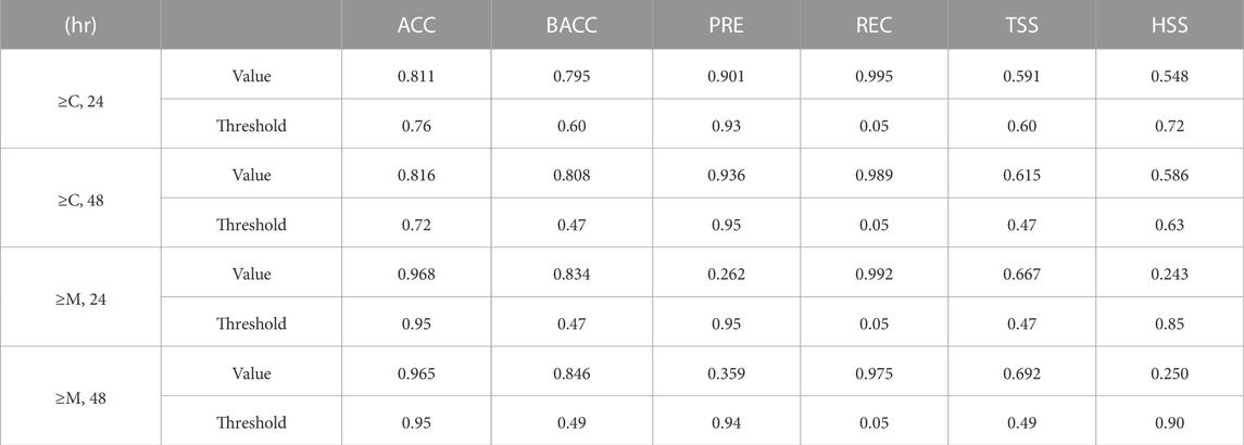
TABLE 5. Maximum Skill Scores by Metric. For each metric and prediction case (flare class and data window), the maximum score achieved by each metric is displayed, along with the threshold yielding that score. This is done separately for each metric and prediction case, and is not our final result.

Balanced accuracy shows a much more useful curve with a peak that is not defined by the class imbalance. For the ≥C-class case, the 24- and 48-h models achieve maximum BACC values of 0.795 and 0.808 at thresholds 0.6 and 0.47, respectively. For the ≥M-class case, the 24-h model reaches BACC = 0.834 with a threshold of 0.47, while the 48-h model reaches BACC = 0.846 with a threshold of 0.49. These thresholds are eventually chosen to optimize overall performance, as depicted by the vertical red lines in Figure 4.

3.1.2 Precision and recall

Across all models, maximum precision values are attained with thresholds near 0.95. The PRE scores for the ≥C-class case are 0.901 for the 24-h case and 0.936 for the 48-h case. These high thresholds and scores are the result of the inherent nature of precision. A high threshold will result in the model only classifying an event as positive when its probability of being severe is extremely high, resulting in extremely reliable positive predictions. This trend can be seen in Figure 4, where precision scores increase almost monotonically. The highest precision scores for the ≥M-class case are 0.262 for the 24-h variation, and 0.359 for the 48-h variation. While these scores occur when the threshold is near 0.95 for the same reason as described in the ≥C-class case, they are significantly lower. This is because there are many more false positives compared to true positives, causing severe predictions to become less reliable.

All four models (≥C with 24 h of data, ≥C with 48 h, ≥M with 24 h, and ≥M with 48 h) attain maximum recall scores when the threshold is 0.05. For the ≥C-class case, scores of 0.995 and 0.989 are reached for the 24-h and 48-h cases, respectively. For the ≥M-class case, the scores are 0.992 and 0.975. While this pattern of extremely high scores at the extremes of the threshold range is similar to that observed in precision, it shows the opposite trend. While precision increases with threshold, recall decreases monotonically. The reason for this is that a low threshold will result in many positive predictions, thereby reducing the number of severe events that the model does not identify, as expressed in a high recall value. Due to the uniform optimization of precision and recall through near-1 and near-0 thresholds, we do not use these metrics to select the optimal threshold.

3.1.3 Heidke skill score and true skill statistic

The ≥ C-class models achieve maximum HSS scores of 0.548 for the 24-h variation (threshold = 0.72) and 0.586 for the 48-h variation (threshold = 0.63). When considering the ≥M-class case, the 24-h model reaches HSS = 0.243 (threshold = 0.85) and the 48-h model reaches HSS = 0.250 (threshold = 0.90). It is observed in Figure 4 that, like the precision curves, the HSS curves are far lower for the ≥M-class case than for the ≥C-class case. A large number of false positives relative to true positives, as seen in Figure 3, may result in this trend. HSS, which is affected by the class imbalance (Woodcock, 1976), is not used in threshold selection.

For the ≥C-class case, the 24- and 48-h models achieve maximum TSS values of 0.591 and 0.615 at thresholds 0.6 and 0.47, respectively. For the ≥M-class case, the 24-h model reaches TSS = 0.667 with a threshold of 0.47, while the 48-h model reaches TSS = 0.692 with a threshold of 0.49.

These optimal thresholds are identical to those of balanced accuracy. TSS is unaffected by the class imbalance (Woodcock, 1976) and is thus used to select the final classification thresholds. TSS has been shown to provide the best metric for flare forecasting performance comparison (Bloomfield et al., 2012). As TSS and BACC are optimized at identical thresholds, the final values chosen reflect the metrics that are unaffected by class imbalance (BACC and TSS).

3.2 Common threshold selection

The selected thresholds are 0.6 for the 24-h ≥ C-class case, 0.47 for the 48-h ≥ C-class case and 24-h ≥ M-class case, and 0.49 for the 48-h ≥ M-class case. This yields the scores shown in Table 6. BACC, REC, and TSS scores are higher for the ≥M-class case than for the ≥C-class case. These metrics all increase with a higher true positive rate, indicating that the models generally misses more ≥C-class flares than ≥ M-class flares. This means that, if a severe flare occurs, the models are more likely to correctly distinguish it from weaker flares if they are trained to recognize ≥M-class flares. For PRE and HSS, the pattern is reversed: performance is significantly higher in the ≥C-class case. This may be explained by the large number of false positives when predicting ≥M-class flares. If the ≥M-class models are more prone to predicting too many examples as positive, it would result in more false positives. This would decrease precision and HSS scores while boosting BACC, REC, and TSS scores (which is also observed). This also explains why precision and HSS scores for the ≥M-class cases are significantly lower than all other scores.

TABLE 6

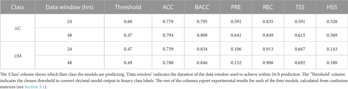
TABLE 6. Experimental Results: Skill Scores.

The skill scores for both the ≥C-class and ≥M-class models show an increase in nearly all metrics when using 48 h of data instead of 24 h. This suggests that there are certain indicators occurring more than 48 h before severe flares that help the model distinguish such regions. The performance increase is slightly larger for the ≥C-class case, suggesting that these indicators are more important in this prediction task when compared to identifying only more powerful flares (≥M). The performance increase is also significantly greater in precision and HSS scores (7%–26% increase instead of $<$5%). The reason for this can be seen in the confusion matrices (Figure 3): increasing the data duration to 48 h dramatically decreases the number of false positives. This means that severe flare predictions become more reliable with larger time windows.

4 Discussion

4.1 Performance comparison

Table 7 displays skill scores for various models developed in prior studies. The most direct comparison can be made with the LSTM model developed by Wang et al. (2020), as they did not use any additional data such as flare history or satellite images. The authors also use 24-h sequences of SHARPs time-series data, but include 20 different SHARPs parameters, as opposed to 18 used in this study. While we randomly select test data, they split the data by year. The authors developed two models with different testing years. Here we compare our results with their highest-performing model. Metrics displayed here are calculated from confusion matrix values. When using the same duration of data (24 h), our model outperforms their LSTM in terms of BACC, REC, and TSS for the ≥C-class case. In terms of accuracy, precision, and HSS, the LSTM outperforms our models. This is consistent with the nature of the metrics: our model has a higher true positive rate, which is naturally accompanied by more false positives. When using TSS to indicate overall performance (Bloomfield et al., 2012), our model achieves better performance overall for the ≥C-class case when using the same data duration. When using 48 h of data instead, our Transformer achieves higher BACC, REC, TSS, and HSS scores. For the ≥M-class case, our 24-h model achieves higher scores only in recall. Using 48 h of data instead, our model compares more favorably, scoring higher in BACC, REC, and TSS. For both the ≥C- and ≥M-class prediction cases, the score increases again demonstrate the positive impact of longer data windows on model performance.

TABLE 7

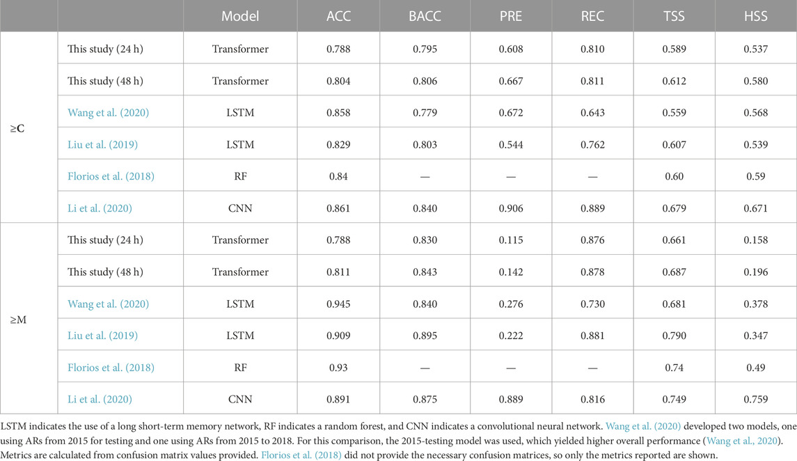
TABLE 7. Comparison with Skill Scores Obtained in Prior Studies.

Liu et al. (2019) used 10-h sequences of 25 physical SHARPs parameters in addition to flare history data to predict flares within 24 h with an LSTM with attention architecture. Flare history parameters enable the model to access information concerning past flares within that active region. This additional data proved to be an important discriminating feature for models that included them, as demonstrated in the feature assessment conducted by the authors. They also used the full data set instead of undersampling the negative class. For the ≥C-class case, our 24-h model outperforms their LSTM only in terms of precision and recall. In this case, their model is better overall when TSS is used as an indicator of overall quality. However, when 48 h of data are used instead, our model demonstrates better performance despite not using flare history data, scoring higher in BACC, PRE, REC, TSS, and HSS. For the ≥M-class case, their model outperforms our Transformers across all metrics, regardless of data window duration.

The random forest (RF) model developed by Florios et al. (2018) also used SHARPs data, but the authors calculated predictors from near-real-time (NRT) LoS magnetograms instead of using definitive SHARPs parameters as model input. NRT data, which are available earlier, can have small differences from definitive data due to lack of certain data correction and calibration steps (Hoeksema et al., 2014). Also unlike the previously compared studies, they do not use data in a time-series format. Because the authors did not provide confusion matrix values, we are only able to compare accuracy, TSS, and HSS. In the ≥C-class case, their RF achieves higher scores than our 24-h model, while our 48-h model scores slightly higher in terms of TSS. For the ≥M-class case, their model outperforms our Transformers for both data durations, with a 12% TSS increase over the 24-h model and an 8% increase over the 48-h model.

Li et al. (2020) attempted the same prediction task with a significantly different approach. The authors used a deep CNN to classify SHARPS LoS magnetograms by whether the ARs observed release a flare of a specific magnitude within 24 h. Like Florios et al. (2018), they do not use a time-series format. The only area where our Transformer models achieve higher performance than the CNN is in terms of recall for both the 24-h and 48-h ≥M-class cases. For the ≥C-class case, their CNN achieves a 15% higher TSS score than our 24-h model and an 11% higher score than our 48-h model. In the ≥M-class case, the CNN scores 13% and 9% higher than our 24- and 48-h Transformers, respectively.

4.2 Conclusion

We develop Transformer networks to predict whether an AR will release a flare of a specific magnitude within 24 h. The model is trained on time-series data consisting of 18 physical parameters that characterize an AR from the Space-weather HMI Active Region Patches (SHARPs) data product, obtained from http://jsoc.stanford.edu/ for ARs from May 2010 through December 2022. After the data are sorted by flare class using the GOES flare catalog and preprocessed, example sequences are generated for each of the four prediction cases: ≥C-class using 24 h of data, ≥C-class using 48 h of data, ≥M-class using 24 h of data, and ≥M-class using 48 h of data. The data are then split randomly, with 80% being used for model training and 20% for testing. After normalization and undersampling of the negative class to yield a balanced data set, the data are prepared for model input. The models used primarily consist of an attention-based Transformer encoder followed by a multi-layer perceptron. Ideal model hyperparameters are chosen through Bayesian optimization, and the classification probability threshold is selected to yield maximum overall performance. The primary conclusions from this study are as follows:

1. The model architecture, which was designed for sequence transduction tasks, is applied to developing a network for time series classification for flare prediction. Model input consists of only 24 or 48 h of time-series SHARPs data, in contrast to the larger time windows, additional parameters, or image data used in prior studies. Data size is further reduced in the undersampling process used to balance the data set.

2. An analysis of model evaluation metrics concludes that of the metrics assessed, the True Skill Statistic (TSS) provides the most accurate information on a model’s predictive value. This is used for probability classification threshold selection and model comparison.

3. Model performance is optimized across all four Transformer models when the threshold (the probability value above which data sequences are classified as positive) is close to 0.5, with slight variations depending on data window length and flare class.

4. For the ≥C-class case, both of our Transformer models outperform a prior study that similarly used comparatively limited data. For the ≥M-class case, our 48-h model performs slightly better while the 24-h model performs slightly worse. When our models are compared to studies that used additional data such as flare history or different data (e.g., satellite images), performance is comparable. For the ≥C-class case, using 48 h of input data for our Transformer network yields higher performance than all prior studies compared that used physical SHARPs parameters.

Our results suggest that Transformer networks are a very promising method of flare forecasting, especially with limited data. Model performance may be improved by using k-fold cross-validation techniques, which were not included in this study due to limited computational resources. In addition, we acknowledge that the reliance on data measurement and calculation accuracy is a weak point across all such machine-learning space weather forecasting methods. Future data including severe flare events may improve model performance due to the rarity of such events in present data sets. Our limited-data approach is conducive to platforms with limited storage such as nanosatellites. In the future, we plan to deploy Transformer networks on a CubeSat platform, where the model will utilize on-board satellite measurements of solar processes to forecast solar flares, thereby providing early warning of severe events.

Data availability statement

The magnetic field data used in this study can be found in the Joint Science Operations Center (JSOC) database: http://jsoc.stanford.edu/. The flare event data used in this study can be found in the GOES X-ray flare catalog provided by the National Centers for Environmental Information: https://www.ngdc.noaa.gov/stp/satellite/goes-r.html. Code files will be made available at https://github.com/keahipelkumdonahue/transformer_flare_forecasting.

Author contributions

KP: Data curation, Formal Analysis, Investigation, Methodology, Software, Supervision, Validation, Visualization, Writing–original draft. FI: Conceptualization, Data curation, Formal Analysis, Investigation, Methodology, Project administration, Resources, Software, Supervision, Validation, Writing–review and editing.

Funding

The author(s) declare financial support was received for the research, authorship, and/or publication of this article. This research was supported by the NOAA cooperative agreements NA17OAR4320101 and NA22OAR4320151.

Acknowledgments

We would like to thank Paul T. M. Loto’ aniu for very helpful suggestions and the SDO/HMI team for their production of the SHARPs data product. KPD would also like to thank Alberto Real for useful discussions and Kira Badyrka for support.

Conflict of interest

The authors declare that the research was conducted in the absence of any commercial or financial relationships that could be construed as a potential conflict of interest.

Publisher’s note

All claims expressed in this article are solely those of the authors and do not necessarily represent those of their affiliated organizations, or those of the publisher, the editors and the reviewers. Any product that may be evaluated in this article, or claim that may be made by its manufacturer, is not guaranteed or endorsed by the publisher.

Author disclaimer

The views, opinions, and findings contained in this report are those of the authors and should not be construed as an official National Oceanic and Atmospheric Administration, National Aeronautics and Space Administration, or other U.S. Government position, policy, or decision.

References

Abduallah, Y., Wang, J. T. L., Wang, H., and Xu, Y. (2023). Operational prediction of solar flares using a transformer-based framework. Sci. Rep. 13, 13665. doi:10.1038/s41598-023-40884-1

PubMed Abstract | CrossRef Full Text | Google Scholar

Bahdanau, D., Cho, K., and Bengio, Y. (2014). Neural machine translation by jointly learning to align and translate. arXiv e-prints , arXiv:1409.0473. doi:10.48550/arXiv.1409.0473

CrossRef Full Text | Google Scholar

Benz, A. O. (2017). Flare observations. Living Rev. Sol. Phys. 14, 2. doi:10.1007/s41116-016-0004-3

CrossRef Full Text | Google Scholar

Bloomfield, D. S., Higgins, P. A., McAteer, R. T. J., and Gallagher, P. T. (2012). Toward reliable benchmarking of solar flare forecasting methods. ApJ 747, L41. doi:10.1088/2041-8205/747/2/L41

CrossRef Full Text | Google Scholar

Bobra, M. G., and Couvidat, S. (2015). Solar flare prediction using SDO/HMI vector magnetic field data with a machine-learning algorithm. ApJ 798, 135. doi:10.1088/0004-637X/798/2/135

CrossRef Full Text | Google Scholar

Bobra, M. G., Sun, X., Hoeksema, J. T., Turmon, M., Liu, Y., Hayashi, K., et al. (2014). The helioseismic and magnetic imager (HMI) vector magnetic field pipeline: SHARPs - space-weather HMI active region Patches. Sol. Phys. 289, 3549–3578. doi:10.1007/s11207-014-0529-3

CrossRef Full Text | Google Scholar

Boureau, Y.-L., Ponce, J., and Lecun, Y. (2010). “A theoretical analysis of feature pooling in visual recognition,” in ICML 2010 - Proceedings, 27th International Conference on Machine Learning, Haifa, Israel, June 21-24, 2010, 111–118.

Google Scholar

Brodersen, K. H., Ong, C. S., Stephan, K. E., and Buhman, J. M. (2010). “The balanced accuracy and its posterior distribution,” in 2010 20th International Conference on Pattern Recognition, Istanbul, Turkey, 23-26 August 2010, 3121–3124. doi:10.1109/ICPR.2010.764

CrossRef Full Text | Google Scholar

Choudhary, D. P., Ambastha, A., and Ai, G. (1998). Emerging flux and X-class flares in NOAA 6555. Sol. Phys. 179, 133–140. doi:10.1023/A:1005063609450

CrossRef Full Text | Google Scholar

Fletcher, L., Dennis, B. R., Hudson, H. S., Krucker, S., Phillips, K., Veronig, A., et al. (2011). An observational overview of solar flares. Space Sci. Rev. 159, 19–106. doi:10.1007/s11214-010-9701-8

CrossRef Full Text | Google Scholar

Florios, K., Kontogiannis, I., Park, S.-H., Guerra, J. A., Benvenuto, F., Bloomfield, D. S., et al. (2018). Forecasting solar flares using magnetogram-based predictors and machine learning. Sol. Phys. 293, 28. doi:10.1007/s11207-018-1250-4

CrossRef Full Text | Google Scholar

Garcia, H. A. (1994). Temperature and emission measure from goes soft x-ray measurements. Sol. Phys. 154, 275–308. doi:10.1007/BF00681100

CrossRef Full Text | Google Scholar

Girdhar, R., Carreira, J. J., Doersch, C., and Zisserman, A. (2019). “Video action transformer network,” in 2019 IEEE/CVF Conference on Computer Vision and Pattern Recognition (CVPR), Long Beach, CA, USA, 15-20 June 2019, 244–253. doi:10.1109/CVPR.2019.00033

CrossRef Full Text | Google Scholar

Hagyard, M. J., Smith, J., Teuber, D., and West, E. A. (1984). A quantitative study relating observed shear in photospheric magnetic fields to repeated flaring. Sol. Phys. 91, 115–126. doi:10.1007/BF00213618

CrossRef Full Text | Google Scholar

Hanssen, A. J., and Kuipers, W. J. (1965). On the relationship between the frequency of rain and various meteorological parameters. Koninklijk Nederlands Meteorologisch Instituut 81, 2–25.

Google Scholar

He, H., and Garcia, E. A. (2009). Learning from imbalanced data. IEEE Trans. Knowl. Data Eng. 21, 1263–1284. doi:10.1109/TKDE.2008.239

CrossRef Full Text | Google Scholar

He, K., Zhang, X., Ren, S., and Sun, J. (2016). “Deep residual learning for image recognition,” in 2016 IEEE Conference on Computer Vision and Pattern Recognition (CVPR), Las Vegas, NV, USA, 27-30 June 2016, 770–778. doi:10.1109/CVPR.2016.90

CrossRef Full Text | Google Scholar

He, X., Tan, E. L., Bi, H., Zhang, X., Zhao, S., and Lei, B. (2022). Fully transformer network for skin lesion analysis. Med. Image Anal. 77, 102357. doi:10.1016/j.media.2022.102357

PubMed Abstract | CrossRef Full Text | Google Scholar

Heidke, P. (1926). Berechnung des erfolges und der güte der windstärkevorhersagen im sturmwarnungsdienst. Geogr. Ann. 8, 301–349. doi:10.1080/20014422.1926.11881138

CrossRef Full Text | Google Scholar

Hoeksema, J. T., Liu, Y., Hayashi, K., Sun, X., Schou, J., Couvidat, S., et al. (2014). The helioseismic and magnetic imager (HMI) vector magnetic field pipeline: overview and performance. Sol. Phys. 289, 3483–3530. doi:10.1007/s11207-014-0516-8

CrossRef Full Text | Google Scholar

Inceoglu, F., Jeppesen, J. H., Kongstad, P., Hernández Marcano, N. J., Jacobsen, R. H., and Karoff, C. (2018). Using machine learning methods to forecast if solar flares will Be associated with CMEs and SEPs. ApJ 861, 128. doi:10.3847/1538-4357/aac81e

CrossRef Full Text | Google Scholar

Inceoglu, F., Pacini, A. A., and Loto’aniu, P. T. M. (2022a). Utilizing AI to unveil the nonlinear interplay of convection, drift, and diffusion on galactic cosmic ray modulation in the inner heliosphere. Sci. Rep. 12, 20712. doi:10.1038/s41598-022-25277-0

PubMed Abstract | CrossRef Full Text | Google Scholar

Inceoglu, F., Shprits, Y. Y., Heinemann, S. G., and Bianco, S. (2022b). Identification of coronal holes on AIA/SDO images using unsupervised machine learning. ApJ 930, 118. doi:10.3847/1538-4357/ac5f43

CrossRef Full Text | Google Scholar

Jarolim, R., Veronig, A. M., Hofmeister, S., Heinemann, S. G., Temmer, M., Podladchikova, T., et al. (2021). Multi-channel coronal hole detection with convolutional neural networks. A&A 652, A13. doi:10.1051/0004-6361/202140640

CrossRef Full Text | Google Scholar

Jonas, E., Bobra, M., Shankar, V., Todd Hoeksema, J., and Recht, B. (2018). Flare prediction using photospheric and coronal image data. Sol. Phys. 293, 48. doi:10.1007/s11207-018-1258-9

CrossRef Full Text | Google Scholar

Kingma, D. P., and Ba, J. (2015). “Adam: a method for stochastic optimization,” in 3rd international conference on learning representations, ICLR 2015. Editors Y Bengio, and Y LeCun.

Google Scholar

Li, X., Zheng, Y., Wang, X., and Wang, L. (2020). Predicting solar flares using a novel deep convolutional neural network. ApJ 891, 10. doi:10.3847/1538-4357/ab6d04

CrossRef Full Text | Google Scholar

Liu, H., Liu, C., Wang, J. T. L., and Wang, H. (2019). Predicting solar flares using a long short-term memory network. ApJ 877, 121. doi:10.3847/1538-4357/ab1b3c

CrossRef Full Text | Google Scholar

Marchetti, F., Guastavino, S., Piana, M., and Campi, C. (2022). Score-oriented loss (SOL) functions. Pattern Recognit. 132, 108913. doi:10.1016/j.patcog.2022.108913

CrossRef Full Text | Google Scholar

Marzban, C. (2004). The ROC curve and the area under it as performance measures. Weather Forecast. 19, 1106–1114. doi:10.1175/825.1

CrossRef Full Text | Google Scholar

Münchmeyer, J., Bindi, D., Leser, U., and Tilmann, F. (2021). Earthquake magnitude and location estimation from real time seismic waveforms with a transformer network. Geophys. J. Int. 226, 1086–1104. doi:10.1093/gji/ggab139

CrossRef Full Text | Google Scholar

Nambiar, A., Heflin, M., Liu, S., Maslov, S., Hopkins, M., Ritz, A., et al. (2023). Transformer neural networks for protein family and interaction prediction tasks. J. Comput. Biol. 30, 95–111. doi:10.1089/cmb.2022.0132

PubMed Abstract | CrossRef Full Text | Google Scholar

Nishizuka, N., Kubo, Y., Sugiura, K., Den, M., and Ishii, M. (2021). Operational solar flare prediction model using Deep Flare Net. Earth, Planets Space 73, 64. doi:10.1186/s40623-021-01381-9

CrossRef Full Text | Google Scholar

Nishizuka, N., Sugiura, K., Kubo, Y., Den, M., and Ishii, M. (2018). Deep flare net (DeFN) model for solar flare prediction. ApJ 858, 113. doi:10.3847/1538-4357/aab9a7

CrossRef Full Text | Google Scholar

Pulkkinen, A., Thomson, A., Clarke, E., and McKay, A. (2003). April 2000 geomagnetic storm: ionospheric drivers of large geomagnetically induced currents. Ann. Geophys. 21, 709–717. doi:10.5194/angeo-21-709-2003

CrossRef Full Text | Google Scholar

Pulkkinen, T. (2007). Space weather: terrestrial perspective. Living Rev. Sol. Phys. 4, 1. doi:10.12942/lrsp-2007-1

CrossRef Full Text | Google Scholar

Raju, H., and Das, S. (2023). Interpretable ML-based forecasting of CMEs associated with flares. Sol. Phys. 298, 96. doi:10.1007/s11207-023-02187-6

CrossRef Full Text | Google Scholar

Ribeiro, F., and Gradvohl, A. L. S. (2021). Machine learning techniques applied to solar flares forecasting. Astronomy Comput. 35, 100468. doi:10.1016/j.ascom.2021.100468

CrossRef Full Text | Google Scholar

Schrijver, C. J. (2007). A characteristic magnetic field pattern associated with all major solar flares and its use in flare forecasting. ApJ 655, L117–L120. doi:10.1086/511857

CrossRef Full Text | Google Scholar

Schwenn, R. (2006). Space weather: the solar perspective. Living Rev. Sol. Phys. 3, 2. doi:10.12942/lrsp-2006-2

CrossRef Full Text | Google Scholar

Srivastava, N., Hinton, G., Krizhevsky, A., Sutskever, I., and Salakhutdinov, R. (2014). Dropout: a simple way to prevent neural networks from overfitting. J. Mach. Learn. Res. 15, 1929–1958. doi:10.3389/fnins.2013.12345

CrossRef Full Text | Google Scholar

Tuli, S., Casale, G., and Jennings, N. R. (2022). TranAD: deep transformer networks for anomaly detection in multivariate time series data. arXiv e-prints , arXiv:2201.07284. doi:10.48550/arXiv.2201.07284

CrossRef Full Text | Google Scholar

Vaswani, A., Shazeer, N., Parmar, N., Uszkoreit, J., Jones, L., Gomez, A. N., et al. (2017). Attention is all you need. arXiv e-prints , arXiv:1706.03762. doi:10.48550/arXiv.1706.03762

CrossRef Full Text | Google Scholar

Wang, X., Chen, Y., Toth, G., Manchester, W. B., Gombosi, T. I., Hero, A. O., et al. (2020). Predicting solar flares with machine learning: investigating solar cycle dependence. ApJ 895, 3. doi:10.3847/1538-4357/ab89ac

CrossRef Full Text | Google Scholar

Woodcock, F. (1976). The evaluation of yes/No forecasts for scientific and administrative purposes. Mon. Weather Rev. 104, 1209–1214. doi:10.1175/1520-0493(1976)104⟨1209:TEOYFF⟩2.0.CO;2

CrossRef Full Text | Google Scholar

Wu, J., Chen, X.-Y., Zhang, H., Xiong, L.-D., Lei, H., and Deng, S.-H. (2019). Hyperparameter optimization for machine learning models based on bayesian optimization. J. Electron. Sci. Technol. 17, 26–40. doi:10.11989/JEST.1674-862X.80904120

CrossRef Full Text | Google Scholar