Resolving the tidal weather of the thermosphere using GDC

NASA’s Geospace Dynamics Constellation (GDC) mission is a six satellite constellation to make in situ measurements of important ionospheric and thermospheric variables to better understand the processes that govern Earth’s near space environment. Scheduled for a 2029 launch into high inclination orbits $\sim 82°$ at $\sim 380$ km, the satellite orbit planes will separate over time to provide almost continuous local solar time coverage every day towards the end of the 3 year baseline GDC mission. As such, the neutral temperature and neutral wind measurements of GDC will likely allow the heliophysics community to make significant progress towards resolving the tidal weather of the thermosphere, that is, day-to-day tidal variability, and how it is driven by meteorological processes near the surface and in situ forcing in the ionosphere-thermosphere system. To assess the GDC ability to accurately resolve the tides each day and when in the mission this can be achieved, we conduct an Observational Simulation System Experiment (OSSE) using SD-WACCM-X and the predicted GDC orbits. Our results show that GDC can provide closure on the tidal variability (mean, diurnal and semidiurnal, migrating and nonmigrating) at orbit height in mission phase 4 and throughout most parts of mission phase 3. We also perform Hough Mode Extension fitting of relevant tidal components to study possible connections between the GDC observations and the tides at 200 km, to assess synergies between GDC and the forthcoming DYNAMIC mission (scheduled to be co-launched with GDC) that will measure altitude-resolved winds and temperatures in the ∼100–200 km height range.

1 Introduction

Each day, upward propagating atmospheric waves carry vast amounts of energy, around 10¹⁶J (Jarvis, 2001), to the ionosphere-thermosphere (IT system). This value is comparable to the input of solar EUV and greater than typical auroral particle and Joule heating combined (Richmond and Lu, 2000; Newell et al., 2009). However, much of the wave spectrum is not well-sampled by observations nor realistically captured in global-scale models, leaving atmospheric waves as one of the largest sources of uncertainty in understanding the variability of the Earth’s upper atmosphere and ionosphere, coupling of the lower and upper atmosphere, and the prediction of the atmosphere’s response to space weather (Sassi et al., 2019). At present, the global-scale wave spectrum is only known in the mesosphere/lower thermosphere (MLT, $<100$ km) and above 250 km, in a limited latitude range equatorward of about 55°, and with a “climatological” time resolution of $>1$ month (Oberheide et al., 2011a) The heliophysics community does not have suitable global measurements in the all-important 100–200 km altitude range, where dissipation and in situ forcing occur. Suitablerefers to the availability of day and nighttime measurements (full local solar time coverage) to resolve the tidal spectrum. Consequently, the 100–200 km altitude region remains the “thermospheric gap” where we know little about the dynamics. Equally important, the “tidal weather,” that is, variability on timescales (days) relevant for space weather, is not known at any altitude above the stratopause up to the exosphere—but is expected to be on the same order as the monthly mean amplitudes as many wave sources are related to meteorological weather near the Earth’s surface Oberheide et al. (2015b).

The importance of resolving the global wave spectrum, particularly the tides, on weather time scales was highlighted by the National Academies in the 2013 Decadal Survey (National Research Council, 2013) which put forward the Geospace Dynamics Constellation (GDC) and the DYNAMIC mission to study the meteorological driving of geospace, among other science questions. GDC is scheduled for a launch in 2029 with all in situ instruments onboard the six identical spacecraft selected. The specifics of the DYNAMIC mission are at the time of this paper not clear as the instruments have not yet been selected—but it is likely that they will include the capability to measure temperatures and winds in the 100–200 km height range, per 2013 Decadal Survey (National Research Council, 2013). We will thus focus on the GDC mission and its ability to resolve the tidal weather in situ around 380 km in the following and only briefly discuss approaches of how to connect GDC and DYNAMIC measurements of tides.

The GDC orbit geometry is complex, to allow measurements to evolve from local to regional to global scales over the course of the 3 year baseline mission (GDC Science and Technology Definition, 2021). In-track and cross-track horizontal winds are prime parameters of GDC, along with neutral temperature and other parameters NNH17ZDA004O-GDC. (2021). Per the NASA ephemeris description GDC Ephemeris. (2022), the GDC satellites will reach a maximum of 6 h local time separation (ascending nodes) in mission phase 3 after 12 months of science operations, 9 h (phase 4) after 22 months and 12 h towards the end of the mission. Science operations will start about 3 months post launch. The maximum local time separation of the spacecraft is unaffected by a potential downscoped (threshold) GDC mission of four spacecraft. In this paper, we conduct an Observational Simulation System Experiment (OSSE) using hourly output of 1 year of 2009 SD-WACCM-X simulations to resolve the mean, diurnal and semdiurnal tidal spectrum every day. Our results show that this is possible with a high level of accuracy during GDC mission phase 4, with degrading capabilities during the earlier parts of the GDC mission.

The manuscript is organized as follows. Section 2 overviews the observational requirements to resolve the tidal weather. Section 3 overviews key aspects of GDC and the SD-WACCM-X simulations and describes the OSSE. Section 4 provides the OSSE results and complements them with the results from the full model as a function of GDC mission phase. Section 5 provides Hough Mode Extension fits to evaluate the connection between GDC and DYNAMIC. Section 6 contains the conclusions.

2 Observational requirements to resolve tidal weather

2.1 Atmospheric tides

Atmospheric tides (Oberheide et al., 2015a) are global-scale oscillations in winds, temperature and many other parameters that attain substantial amplitudes (several tens of m/s, K) in the mesopause region around 90 km and above in the thermosphere. The most important tidal periods (in this order) are harmonics of a solar day: diurnal (24 h), semidiurnal (12 h), terdiurnal (8 h) and quarterdiurnal (6 h). Tides can propagate westward, eastward or remain stationary with horizontal wavelengths (along longitude) of order $\sim \mathrm{10,000}$ km, vertical wavelengths between ten to several hundred kilometers, and substantial changes in magnitude as function of latitude. Many tidal components are forced in the troposphere, through infrared absorption by tropospheric water vapor and latent heat release during cloud droplet formation in organized deep convective systems. As such, tides are more than likely to map surface weather variability into the space weather of the ionosphere: either through direct upward propagation into the thermosphere or through dynamo processes in Earth’s E-region with subsequent mapping of polarization electric fields along magnetic field lines into the F-region (Immel et al., 2006; Forbes et al., 2009). The new COSMIC-2 constellation allows one to diagnose F-region plasma density tides every day (Oberheide, 2022) and shows that weather-like tidal plasma variations are ubiquitous. Further tidal sources are in the stratosphere/mesosphere, through ultraviolet absorption by ozone and several nonlinear fluid dynamical processes, and in the thermosphere, through far and extreme ultraviolet absorption and through interactions of the fluid with ions (Hagan et al., 2001; Häusler et al., 2013; Jones Jr. et al., 2013). An additional, poorly understood, pathway is the dissipation of convectively forced gravity waves that, according to modeling, produces body forces and heating in the 170–200 km altitude range that in situ force a spectrum of nonmigrating tides Vadas et al. (2014). In order to separate tidal variability imposed by surface weather from variability driven by nonlinearity, and solar and geomagnetic forcing from above, one needs to obtain the spectrum the tides on weather timescales (ideally, day-to-day).

The general form of a tidal oscillation at a particular latitude φ and altitude z is given in Eq. 1 and a wave crest occurs when Eq. 2 is satisfied.

$A\cos \left(s\lambda -{\sigma }_{m}t-\mathrm{\Phi }\right)(1)$

$\mathrm{\Phi }=s\lambda -{\sigma }_{m}t(2)$

A = A(φ, z) is the tidal amplitude, Φ = Φ(φ, z) is the tidal phase, t is universal time, λ is longitude, s ≥ 0 is the zonal wavenumber (the number of wave crests that occur along a latitude circle) and σ_m is the tidal frequency. The wave propagates eastward (or remains standing for s = 0) for σ_m > 0 and westward for σ_m < 0. Using σ₁ = (2π/24) hour⁻¹ for the diurnal base frequency, the mth diurnal harmonic is expressed as σ_m = mσ₁, with m = [±1, ±2, ±3, ±4] for diurnal, semidiurnal, terdiurnal, quarterdiurnal tides, respectively. Eq. 1 expressed in local solar time (LST, the natural time frame of reference of a satellite in low Earth orbit, t_LST = t + λ/σ₁) is as follows.

$A_{m,s}\cos \left(\left(s+m\right)\lambda -{\sigma }_m{t}_{\mathit{LST}}-{\mathrm{\Phi }}_{m,s}\right)(3)$

Amplitude and phase depend on frequency and zonal wavenumber, now indicated by the m, s subscripts. Tides are ubiquitous and usually a whole spectrum of different tidal components (that is, (m, s) frequency/wavenumber pairs) is simultaneously excited. Their linear superposition (Eq. 4) is what is observed.

${\displaystyle \sum _{m,s}}{A}_{m,s}\cos \left(\left(s+m\right)\lambda -{\sigma }_m{t}_{\mathit{LST}}-{\mathrm{\Phi }}_{m,s}\right)(4)$

An important subset of the tides follow the apparent (from a ground-based observer perspective) westward motion of the Sun. For these so-called migrating tides, s = −m, m < 0 and Eq. 3 simplifies to

$A_{-|m|,|m|}\cos \left(|m|{\sigma }_1{t}_{\mathit{LST}}-{\mathrm{\Phi }}_{-|m|,|m|}\right)(5)$

Eq. 5 shows that migrating tides have the same local solar time variation at all longitudes. The tide is called migrating diurnal tide if (m, s) = (−1, 1), migrating semidiurnal tide if (m, s) = (−2, 2), migrating terdiurnal tide if (m, s) = (−3, 3) and so on. Tidal components with s ≠ − m are called nonmigrating tides. Tidal components are usually identified by a two-letter, one-number nomenclature: the first letter indicates the period (“D”: diurnal 24 h, “S”: semidiurnal 12 h, “T”: terdiurnal 8 h, “Q”: quarterdiurnal 6 h), the second letter is the propagation direction (“W”: westward, “E”: eastward, “S”: standing), and the number is the zonal wavenumber s. With that, the migrating semidiurnal tide (m, s) = (−2, 2) is SW2, the nonmigrating diurnal eastward propagating tide of zonal wavenumber 3 (m, s) = (1, 3) is DE3, and so on.

2.2 Observational requirements

The key science requirement is to attain wind and temperature data that allow one to diagnose the tidal spectrum (m, s) as a function of latitude and altitude, for periods m = [±1, ±2, ±3, ±4] = [±24, ±12, ±8, ±6] hours and zonal wavenumbers s = [0, 6], and to do so on a daily basis. Harmonic fitting (Fourier decomposition) of Eq. 4 requires full local solar time and longitude coverage to delineate the tidal amplitudes A_m,s and phases Φ_m,s as function of latitude and altitude. The longitude coverage requirement makes global observations from space essential, as a single ground-based instrument cannot separate between different zonal wavenumbers s. Suitable networks of ground-based instruments are not feasible due to the land/ocean distribution on Earth. The local solar time coverage requirement can been achieved by making use of spacecraft local solar time precession, that is, combining several weeks of observations into a “composite day” that covers all local solar times. However, this puts a severe limitation on the time resolution of tidal diagnostics from a single spacecraft. At any given latitude, a single spacecraft observes at two different local solar times each day: one on the ascending orbit node and one on the descending orbit node. These local solar times are largely independent of longitude (variations for a given day and orbit node are within a few minutes) and change from 1 day to another by several minutes towards earlier times, depending on orbit inclination.

For example, a single spacecraft in a 82° inclination orbit needs about 90 days for the ascending orbit node to precess 12 h in local solar time, which can easily be computed from first principles (Nielsen et al., 1958). The 12-h descending orbit node precession is 90 days, too. Consequently, one would need to combine 90 days of observations (for 82° inclination) to obtain the “composite day” 24 h local solar time coverage needed to diagnose A_m,s and Φ_m,s. Consequently, the time resolution of current state-of-the-art tidal diagnostics in the mesosphere/lower thermosphere region is 61 days (TIMED satellite) (Oberheide et al., 2006; Forbes et al., 2008), 41 days (low latitudes, ICON satellite) (Cullens et al., 2020; Forbes et al., 2022) and 135 days around 400 km (CHAMP satellite, inclination 87.3°) (Häusler and Lühr, 2009). Attempts to diagnose short-term tidal variability from a single satellite, without exceptions, rely on assumptions such as neglecting certain (m, s) pairs, setting in situ sources to zero, or others (Oberheide et al., 2002; Oberheide et al., 2015b; Lieberman et al., 2013; Pedatella et al., 2016; Gasperini et al., 2020). Such assumptions may be justified for certain altitude regimes and situations, for example, when multiple data sources indicate the predominance of a certain (m, s) tidal component, but become increasingly questionable, even speculative, throughout the thermosphere because of a lack of observations. The only solution to the problem is to increase the number of local solar times observed each day by flying multiple spacecraft in different orbital planes, as in the GDC constellation.

3 GDC, SD-WACCM-X, and OSSE

3.1 GDC

The six GDC satellites (numbered GDC-1 to GDC-6) will be launched into circular orbits at about 380 km and approximately 82° inclination, with some slight variations in the inclination between the different spacecraft to allow for differential orbit precession and thus a spreading of local solar time (LST) over the lifetime of the mission (Figure 1). As already mentioned in section 2, the LST for a given day, orbit node and latitude is almost longitude independent. Neutral temperatures and winds will be measured by the MoSAIC instrument onboard each satellite with a Program Element Appendix (PEA) (NNH17ZDA004O-GDC, 2021) expected performance of accuracy/precision of 20/10 m/s (winds) and 10/2% (temperature), and a cadence of 3 s. Further details of the MoSAIC instrument are beyond the scope of this paper and the reader is referred to future literature once the specifics of the instrument have been made public. The GDC ephemeris files (revision C) provided by NASA (GDC Ephemeris, 2022) assume a first mission day of 31 July 2028 and an end of mission on 30 April 2031, for a total of 1,003 days every 30 s “Mission day” is defined as day of science operations (starting with GDC phase 1) and excludes the approximately 3 months of commissioning after launch.

FIGURE 1

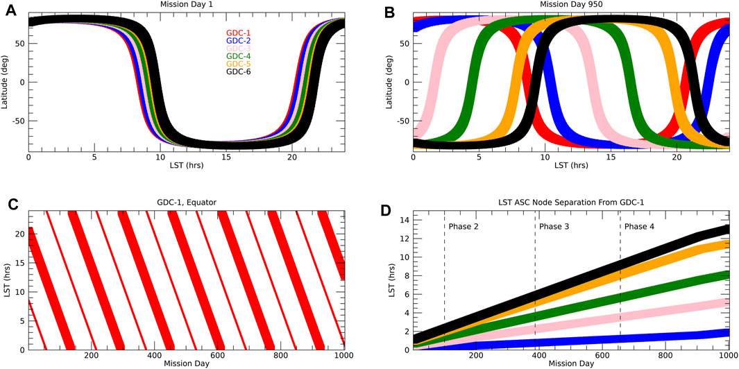
FIGURE 1. (A) Local solar time of the six GDC spacecraft as function of latitude for mission day 1. Mission day is relative to the beginning of GDC mission phase 1, about 3 months after launch. (B) Same as (A) but for mission day 950. (C) Local solar time precession of GDC-1 over the mission. Large symbols indicate ascending orbit nodes and small symbols indicate descending orbit nodes. (D) Local solar time separation between the spacecraft as function of mission day. Plotted is the difference for the ascending orbit node relative to GDC-1 with the same color code as in (A).

GDC has four phases for its science operations with phase 1 marking the beginning of full science operations. In phase 1, the orbital planes of the six spacecraft (and hence their LST of measurement) are close together, followed by phases 2, 3, and 4 with a more or less linear increase in LST separation. See Figure 1 for a high level summary of LST versus latitude toward the beginning and the end of the mission, and the evolution of LST over time, with the LST of the spacecraft ascending orbit nodes distributed over 12 h towards the end of the mission. Along with the descending orbit nodes, full LST coverage is achieved every day over most parts of phase 4. The GDC phases are further subdivided depending on where the spacecraft are placed on each orbit relative to each other, to optimize coverage for the local, regional, and global science objectives. The relative placement of the spacecraft on each orbit does not matter for the tides (but is accounted for in the OSSE) and the reader is referred to the NASA documentation (GDC Ephemeris, 2022) for further details. Figure 2A exemplifies the typical single day coverage of one GDC spacecraft, here shown as sampled SD-WACCM-X zonal winds. The equatorial LST coverage of the six spacecraft for the 40 days following mission day 950 towards the very end of phase 4 is shown in Figure 2B. Almost full local solar time coverage is maintained even in case of a four spacecraft threshold mission that consists of the removal of the GDC-3 and GDC-5 spacecraft (NNH17ZDA004O-GDC, 2021).

FIGURE 2

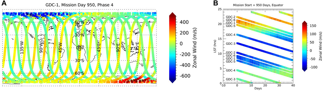
FIGURE 2. (A) Zonal wind from SD-WACCM-X sampled along the orbit track of GDC-1 for mission day 950. (B) Equatorial (±2.5° latitude) local solar time coverage and evolution of the six GDC spacecraft starting on mission day 950 with sampled zonal wind from SD-WACCM-X.

3.2 SD-WACCM-X

The Whole Atmosphere Community Climate Model with thermosphere-ionosphere eXtension (WACCM-X) is a whole atmosphere model extending from the surface to the upper thermosphere (4.1*10^–10 hPa, 500–700 km depending on solar activity) (Liu et al., 2018). The horizontal resolution is 1.9 ° × 2.5 ° (lat × lon). The vertical resolution is variable, and is 0.25 scale heights above 0.96 hPa, with a finer resolution at lower altitudes. The ‘Specific-Dynamics’ or SD-WACCM-X version nudges MERRA-2 data up to 60 km (Smith et al., 2017). The ionosphere and thermosphere processes are largely adopted from TIEGCM. Solar and geomagnetic forcing are parameterized by F10.7 cm and either Kp or solar wind parameters. In the following, we use 1-hourly model output for the year 2009.

3.3 OSSE

The Observational Simulation System Experiment (OSSE) can be thought of as “flying the GDC spacecraft through the model,” followed by a tidal diagnostic approach that would be applied in the same way once real data are available. The same 2009 SD-WACCM-X simulation was used throughout the OSSE. For example, 31 December 2029 in the ephemeris file would use 31 December 2009 from the model, and 1 January 2030 would use 1 January 2009; and so on.

“Flying the GDC spacecraft through the model” is a two step process and essentially a linear interpolation. First, the vertical pressure coordinate in the model is replaced by the daily mean, global mean geopotential height. Second, the longitude, latitude and altitude of each spacecraft is read from the ephemeris files (provided every 30 s) and the model temperature, zonal wind and meridional wind (T, u, v) at the model height closest to the spacecraft altitude are linearly interpolated in longitude, latitude and time, resulting in daily maps of GDC-sampled SD-WACCM-X such as exemplified in Figure 2A for GDC-1. Note that the anticipated T, u, v data from GDC will have a factor of 10 more data along the orbit track if their cadence is 3 s as prescribed by the PEA (NNH17ZDA004O-GDC, 2021). This, however, does not impact the results of our study because the 30 s sampling used reflects the approximate model resolution and because of the global scale (1,000 s of km) of the tides.

The tidal diagnostic is also a two step process, composed of mapping T, u, v from the combined six spacecraft on a regular longitude × latitude × local solar time grid (5 ° × 5 ° × 1h) each day, followed by two-dimensional Fourier diagnostic to obtain the tidal amplitudes and phases as function of period, propagation direction and zonal wavenumber. First, the daily data of each spacecraft, separately for ascending and descending orbit nodes, are combined into ± 2.5° latitude bins every 5°, sorted in longitude and then brought on a regular 5° longitude grid through harmonic regression (zonal wavenumber 0–6). When repeated for all six spacecraft, this results in regularly gridded (longitude and latitude) T, u, v fields at 12 different (but at irregular intervals) local solar times. Then, harmonic regression in local solar time (mean, diurnal, semidiurnal, terdiurnal, quaterdiurnal) is applied and one obtains T, u, v on a regular longitude × latitude × local solar time grid (5 ° × 5 ° × 1h). Second, the tidal spectrum at each latitude is easily obtained through standard 2D (local solar time, longitude) Fourier fitting.

The most critical part in our OSSE is the local solar time separation of the six GDC spacecraft because of the need for full (24 h) LST coverage to perform the 2D Fourier fitting. If the LSTs of the six spacecraft are well separated (i.e., Figure 2B), the harmonic regression in LST will work well. However, if the LSTs are not well separated, i.e., in the earlier parts of the mission (Figure 1), the regression will not work well and the resulting spectra will be aliased. The quality of the OSSE results, and thus the GDC ability to resolve the tidal weather of the thermosphere, can easily be assessed by comparing with the amplitudes and phases from the full model (the “truth”), which are straightforwardly computed using 2D Fourier analysis.

4 Results

In the following, we focus on temperature and a subset of two migrating (DW1, SW2) and two nonmigrating (DW2, SE2) tidal components and the mean. Results for other tidal temperature components above the noise level and representative zonal and meridional wind tides can be found in the Supplementary Material. DW2 and SW2 are the two biggest tides, while SE2 largely originates from tropospheric weather (Oberheide et al., 2011b), and DW2 is, according to theory, in situ forced in the high latitude thermosphere above 200 km through ion drag (Jones et al., 2013).

4.1 End of phase 4

The maximum LST spread is achieved towards the end of phase 4. Figures 3–7 show the evolution of amplitudes and phases from the OSSE (left column) versus the model “truth” (right column). Agreement is within one color scale and full recovery of the tidal weather at all latitudes and the mean can be achieved. A similar level of agreement is found for the wind tides and the other tidal components shown in the supplement.

FIGURE 3

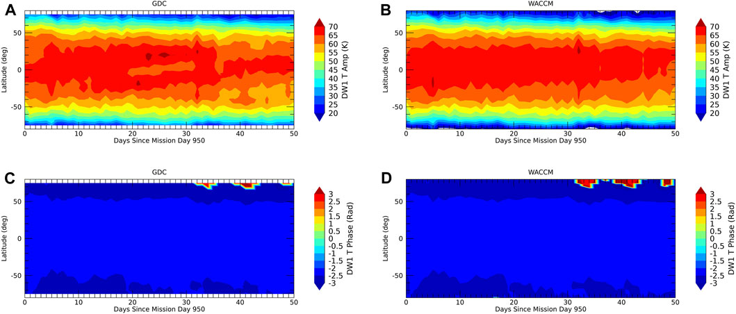
FIGURE 3. DW1. (A) GDC OSSE temperature amplitudes towards the very end of phase 4. (B) Same as (A) but from the full SD-WACCM-X model. (C) GDC OSSE temperature phases (rad, maximum at 0° longitude). (D) Same as (C) but from the full SD-WACCM-X model.

FIGURE 4

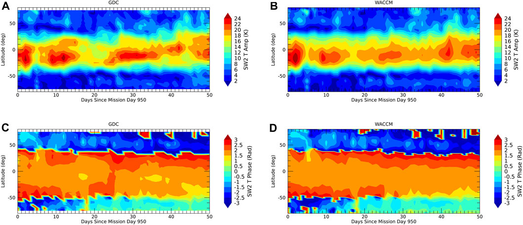
FIGURE 4. Same as Figure 3 but for SW2.

FIGURE 5

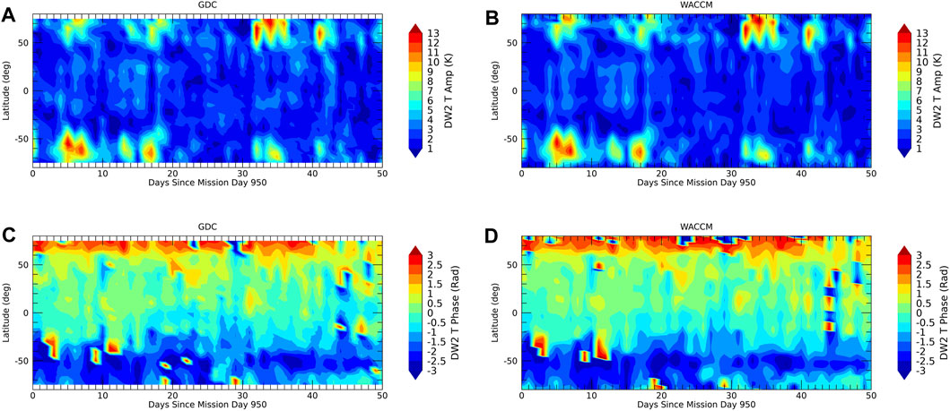
FIGURE 5. Same as Figure 3 but for DW2.

FIGURE 6

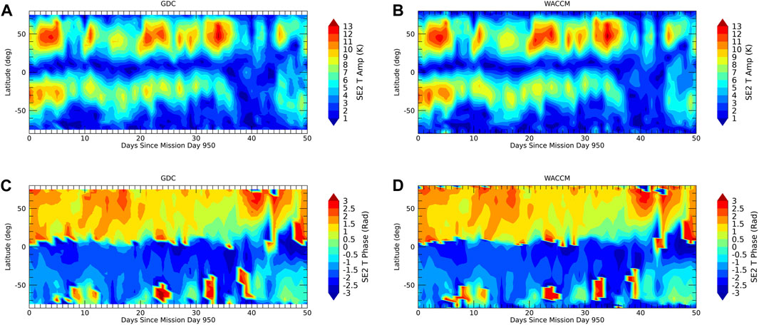
FIGURE 6. Same as Figure 3 but for SE2.

FIGURE 7

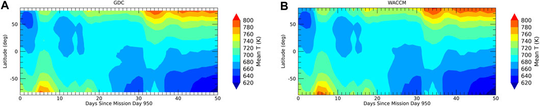
FIGURE 7. Same as Figure 3 but for the mean and without phases.

4.2 Early phase 3 to end of phase 4

To study the impact of decreasing local solar time separation between the spacecraft, it is sufficient to study the differences between the OSSE and the “truth” at peak latitudes. This is shown in Figure 8 for DW2, DE3, DW2, SW2, SE2, and the mean for differences in Kelvin, and the 30-day running mean standard deviation of the differences relative to the 30-day running mean SD-WACCM-X amplitude in percent. In phase 4, differences are well within 1 K, with the exception of DW1 which can reach up to 4 K. However, the migrating tides DW1 and SW2 can be recovered within 5% during phase 4 and within 10% during phase 3 (including the early phase 3). The two eastward propagating DE3 and SE2 components can be recovered within 10–15% between the middle of phase 3 to the end of the mission. In early phase 3, the quality of the recovery rapidly decreases. DW2 is recovered within 20% during phase 4 and the last 2 months of phase 3 but not in earlier phases. The recovery of the mean is possible through phases 3 and 4, albeit with a somewhat larger error in the first half of phase 3. As a general finding, tidal recovery after mission day 600 (late phase 3) works well with increasing errors before that time with the specifics of the latter depending on the tidal component. Tidal diagnostics in phases 1 and 2 are not feasible on a day-to-day basis although combining several days/weeks of data might help to obtain tidal definitions on time scales shorter than the orbit precession period. This is, however, beyond the scope of the current study.

FIGURE 8

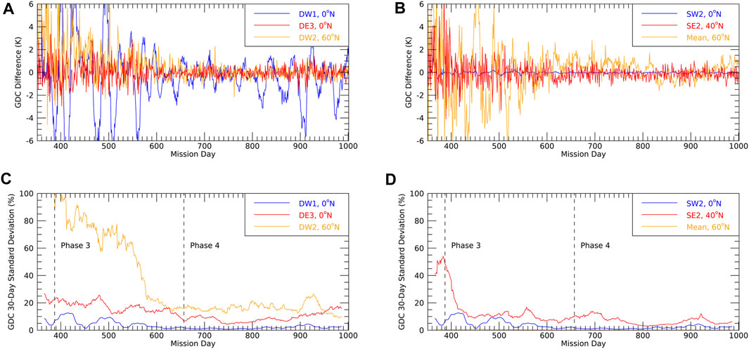
FIGURE 8. Tidal weather recovery during phases 3 and 4. (A) Difference between GDC and SD-WACCM-X amplitudes at peak latitudes in Kelvin: DW1, DE3, DW2. (B) As in (A) but for SW2, SE2, mean. (C) 30-day running mean standard deviation of (A) relative to the 30-day running mean SD-WACCM-X amplitude in percent. (D) As in (C) but for SW2, SE2, mean.

5 Hough mode extension fits

Hough Mode Extensions (HME, Lindzen et al. (1977)) are modifications of the classical tidal theory to describe the latitude/altitude variation of upward propagating tides by accounting for dissipative processes that make the tidal equation inseparable. HMEs are computed using a linear tidal model and can be thought of as forming a complex vector space onto which tidal amplitudes and phases are projected by fitting the HMEs to observed tides in a given latitude/altitude range. The HMEs then provide the tidal amplitudes and phases at all latitudes and all altitudes, even those that have not been observed. The approach has been extensively used in the past to study upward propagation of tides from TIMED and ICON observations (Oberheide and Forbes, 2008; Oberheide et al., 2011a; Kumari and Oberheide, 2020; Forbes et al., 2022), and validated with CHAMP (Forbes et al., 2009; Häusler et al., 2013), HRDI and WINDII (Lieberman et al., 2013) and ground-based observations (Yuan et al., 2014). On the other hand, differences between in situ observations around 400 km with HME fit results to TIMED tidal temperatures and winds in the mesosphere/lower thermosphere were used to predict the existence of tidal sources in the thermosphere (Oberheide et al., 2009), i.e., through ion drag, that have by now been reproduced in dedicated general circulation model simulations (Jones Jr. et al., 2013).

In general, one can use HMEs to connect the in situ GDC observations with the tides in the 100–200 km height region of the atmosphere targeted by the DYNAMIC mission put forward in the 2013 Decadal Survey (National Research Council, 2013). As of this day, NASA plans to launch DYNAMIC at the same time as GDC, to do concurrent measurements (NNH23ZDA0190, 2023). HME fits to GDC will thus allow one to downward extend tides to 200 km and compare with DYNAMIC tides: a structurally good agreement would indicate that no thermospheric sources between 200–380 km exist and conclusively connect upward propagating tides from mostly tropospheric/stratospheric sources to GDC. If larger differences exist, they would indicate the presence of thermospheric sources, an important result on its own. To test this approach, we perform a number of HME fits to 380 km tides for GDC mission phase 4 utilizing the HMEs described by Forbes and Zhang. (2022) for solar minimum conditions (F10.7 cm = 75 sfu). For simplicity, the fits are performed on the SD-WACCM-X full model temperature tides, which is sufficient because of the close agreement between the GDC OSSE and the full model tides.

To exemplify the approach, Figure 9 shows an example for SE2, a tidal component with no known sources in the thermosphere that largely originates from latent heat release in deep convective systems in the tropical troposphere. HME fits to SE2 from TIMED observations have been shown to agree well with CHAMP in situ tidal diagnostics (Oberheide et al., 2011b). The fit results in the left column use the first six HMEs for SE2 (Forbes and Zhang, 2022), for F10.7 cm = 75 sfu, fitted between ± 65° latitude and at 380 km altitude. To demonstrate the height structure, panel a) shows a day when the amplitudes were particularly large. The comparison with the full SD-WACCM-X amplitudes in panel c) indicates that the HME approach reproduces the “truth” fairly well down to approximately 200 km where the notional Decadal Survey DYNAMIC mission (National Research Council, 2013) would measure. This is also reflected in the good agreement between the HME and full model time evolutions at 380 km and 200 km, shown in panels c) to f). Larger differences start to emerge below 200 km due to the presence of higher order (shorter vertical wavelength) modes that dissipate more quickly when propagating upward: the latter cannot be accurately captured when fitting to 380 km altitude. There is also a high southern latitude amplitude maximum in the full model output that is not captured by the HMEs, indicating the presence of some in situ tidal forcing processes in the thermosphere, possibly related to ion drag. Overall, HMEs will be able to connect GDC and DYNAMIC tidal diagnostics for components that have no thermospheric sources, such as SE2, DE3 (not shown) and others, and close the 200–380 km measurement gap between the two missions.

FIGURE 9

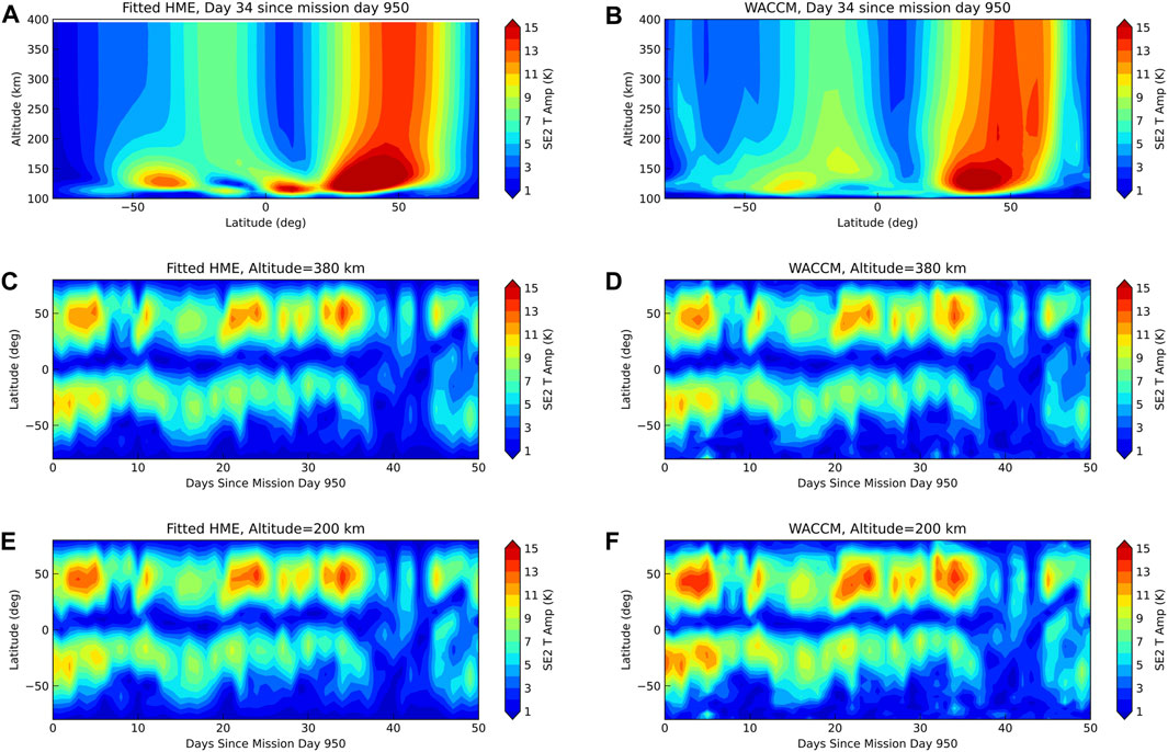
FIGURE 9. SE2. (A) Fitted HME amplitude for day 34 (since mission day 950). (B) As in (A) but from the full SD-WACCM-X model. (C) Fitted HME amplitude evolution at 380 km. (D) As in (C) but from the full SD-WACCM-X model. (E) Fitted HME amplitude evolution at 200 km. (F) As in (E) but from the full SD-WACCM-X model.

A more complicated case is shown in Figure 10 for the SW2 component. SW2 in the thermosphere comes partly from upward propagation from the lower atmosphere and partly from in situ solar forcing with significantly different relative contributions at different altitudes due to forcing and dissipation (Forbes et al., 2011). As such, large differences between the HME fits and the full model exist below 200 km and also at higher latitudes between 200–380 km. Altitude-varying in situ forcing is not well-captured by HME fits, particularly at high latitudes, i.e., the 70°N amplitude maximum around 200 km in the full model is missing in the HME fits, with HMEs producing generally much to large signals below 150 km. Only low latitude in situ forced SW2 projects well into the HMEs in the 200–380 km range, producing the good temporal evolution agreement at low latitudes shown in panels c) to f). Consequently, the low latitude SW2 measured by DYNAMIC could be interpreted as the main source of the low latitude SW2 from GDC. Differences at high latitudes, however, persist and the HMEs would help to isolate the parts of the SW2 where additional tidal forcing and/or changes in tidal dissipation occur in the altitude range between DYNAMIC and GDC. This is particularly interesting for components such as DW2 and D0 that are hypothesized to come from high latitude ion drag forcing above 200 km (Jones Jr. et al., 2013) or from gravity wave dissipation around 200 km at low to mid latitudes (Vadas et al., 2014). DW2 and D0 from HME fits at 380 km (not shown) are quite small while the full model (Figure 5) shows large amplitudes at high latitudes (in situ forcing through GW dissipation is not fully captured in SD-WACCM-X due to the model resolution).

FIGURE 10

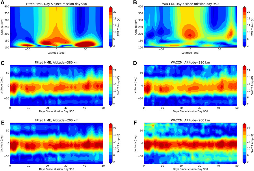
FIGURE 10. As Figure 9 but for the SW2 component.

6 Conclusion

Our Observational Simulation System Experiment using SD-WACCM-X and the predicted GDC orbits demonstrate that GDC can resolve the day-to-day tidal variability (mean, diurnal and semidiurnal, migrating and nonmigrating) at orbit height in mission phase 4 and throughout most parts of mission phase 3. The quality of high latitude tidal recovery starts to deteriorate before mission day 600, about 2 months before the end of phase 3. We note that the mean state of thermosphere can also be recovered on a day-to-day basis throughout phases 3 and 4, including the mean meridional circulation. A more detailed study that includes Monte-Carlo simulations of measurement errors has to await final specifications of the instruments onboard GDC. However, the 3 s cadence of the wind and temperature measurements on each spacecraft and the 5° latitude binning used in the tidal diagnostics would produce approximately 3,600 data points each day for a given latitude bin that enter the further gridding on longitude and local solar time (15 orbits, six spacecraft, ascending and descending orbit nodes, 20 data points along track within 5°; 15 × 6 × 2 × 20 = 3,600). It is thus reasonable to predict that a targeted (NNH17ZDA004O-GDC, 2021) wind precision of 10 m/s and temperature precision of 2% (20 K) will result in amplitude errors that are well within 1 m/s (1 K). Our Hough Mode Extension fitting of relevant tidal components to GDC further supports the concept to fly GDC and DYNAMIC concurrently, with DYNAMIC capable of informing GDC about the sources of the observed tidal variability and for the capability of the combined measurements to further test current theories of in situ tidal forcing and dissipation.

Data availability statement

The datasets presented in this study can be found in online repositories. The names of the repository/repositories and accession number(s) can be found in the article/Supplementary Material.

Author contributions

JO: Conceptualization, Data curation, Formal Analysis, Funding acquisition, Investigation, Methodology, Project administration, Resources, Software, Supervision, Validation, Visualization, Writing–original draft, Writing–review and editing. SG: Formal Analysis, Investigation, Software, Visualization, Writing–review and editing. MN: Formal Analysis, Investigation, Software, Visualization, Writing–review and editing.

Funding

The author(s) declare financial support was received for the research, authorship, and/or publication of this article. JO and SG were partly supported through NASA grant 80NSSC22-K0018.

Conflict of interest

The authors declare that the research was conducted in the absence of any commercial or financial relationships that could be construed as a potential conflict of interest.

Publisher’s note

All claims expressed in this article are solely those of the authors and do not necessarily represent those of their affiliated organizations, or those of the publisher, the editors and the reviewers. Any product that may be evaluated in this article, or claim that may be made by its manufacturer, is not guaranteed or endorsed by the publisher.

Supplementary material

The Supplementary Material for this article can be found online at: https://www.frontiersin.org/articles/10.3389/fspas.2023.1282261/full#supplementary-material

References

Cullens, C. Y., Immel, T. J., Triplett, C. C., Wu, Y. J., England, S. L., Forbes, J. M., et al. (2020). Sensitivity study for icon tidal analysis. Prog. Earth Planet. Sci. 7, 18. doi:10.1186/s40645-020-00330-6

PubMed Abstract | CrossRef Full Text | Google Scholar

Forbes, J. M., Bruinsma, S. L., Zhang, X., and Oberheide, J. (2009). Surface-exosphere coupling due to thermal tides. Geophys. Res. Lett. 36, 38748. doi:10.1029/2009GL038748

CrossRef Full Text | Google Scholar

Forbes, J. M., Oberheide, J., Zhang, X., Cullens, C., Englert, C. R., Harding, B. J., et al. (2022). Vertical coupling by solar semidiurnal tides in the thermosphere from icon/mighti measurements. J. Geophys. Res. Space Phys. 127, e2022JA030288. doi:10.1029/2022ja030288

CrossRef Full Text | Google Scholar

Forbes, J. M., Zhang, X., Bruinsma, S., and Oberheide, J. (2011). Sun-synchronous thermal tides in exosphere temperature from CHAMP and GRACE accelerometer measurements. J. Geophys. Res. Space Phys. 116, 16855. doi:10.1029/2011JA016855

CrossRef Full Text | Google Scholar

Forbes, J. M., and Zhang, X. (2022). Hough mode Extensions (HMEs) and solar tide behavior in the dissipative thermosphere. J. Geophys. Res. Space Phys. 127, e2022JA030962. doi:10.1029/2022ja030962

CrossRef Full Text | Google Scholar

Forbes, J. M., Zhang, X., Palo, S., Russell, J., Mertens, C. J., and Mlynczak, M. (2008). Tidal variability in the ionospheric dynamo region. J. Geophys. Res. Space Phys. 113, 12737. doi:10.1029/2007JA012737

CrossRef Full Text | Google Scholar

Gasperini, F., Liu, H., and McInerney, J. (2020). Preliminary evidence of madden-julian oscillation effects on ultrafast tropical waves in the thermosphere. J. Geophys. Res. Space Phys. 125, e2019JA027649. doi:10.1029/2019ja027649

CrossRef Full Text | Google Scholar

GDC Ephemeris (2022). GDC design reference mission predicted ephemeris description, revision C. Tech. rep., NASA.

Google Scholar

GDC Science and Technology Definition (2021). Final report. Tech. rep., NASA.

Google Scholar

Hagan, M. E., Roble, R. G., and Hackney, J. (2001). Migrating thermospheric tides. J. Geophys. Res. Space Phys. 106, 12739–12752. doi:10.1029/2000JA000344

CrossRef Full Text | Google Scholar

Häusler, K., and Lühr, H. (2009). Nonmigrating tidal signals in the upper thermospheric zonal wind at equatorial latitudes as observed by CHAMP. Ann. Geophys. 27, 2643–2652. doi:10.5194/angeo-27-2643-2009

CrossRef Full Text | Google Scholar

Häusler, K., Oberheide, J., Lühr, H., and Koppmann, R. (2013). “The geospace response to nonmigrating tides,” in Climate and weather of the sun-earth system (CAWSES): Highlights from a priority Program. Editor F. J. Lübken (Dordrecht, Heidelberg, New York, London: Springer Atmospheric Sciences), 481–550. doi:10.1007/978-94-007-4348-9

CrossRef Full Text | Google Scholar

Immel, T. J., Sagawa, E., England, S. L., Henderson, S. B., Hagan, M. E., Mende, S. B., et al. (2006). Control of equatorial ionospheric morphology by atmospheric tides. Geophys. Res. Lett. 33, L15108. doi:10.1029/2006GL026161

CrossRef Full Text | Google Scholar

Jarvis, M. J. (2001). Bridging the atmospheric divide. Science 293, 2218–2219. doi:10.1126/science.1064467

PubMed Abstract | CrossRef Full Text | Google Scholar

Jones, M., Forbes, J. M., Hagan, M. E., and Maute, A. (2013). Non-migrating tides in the ionosphere-thermosphere: in situ versus tropospheric sources. J. Geophys. Res. Space Phys. 118, 2438–2451. doi:10.1002/jgra.50257

CrossRef Full Text | Google Scholar

Kumari, K., and Oberheide, J. (2020). QBO, ENSO, and solar cycle effects in short-term nonmigrating tidal variability on planetary wave timescales from saber—an information-theoretic approach. J. Geophys. Res. Atmos. 125, e2019JD031910. doi:10.1029/2019jd031910

CrossRef Full Text | Google Scholar

Lieberman, R. S., Oberheide, J., and Talaat, E. R. (2013). Nonmigrating diurnal tides observed in global thermospheric winds. J. Geophys. Res. Space Phys. 118, 7384–7397. doi:10.1002/2013JA018975

CrossRef Full Text | Google Scholar

Lindzen, R. S., Hong, S. S., and Forbes, J. (1977). Semidiurnal Hough mode extensions in the thermosphere and their application. Washington, DC: Naval Research Laboratory.

Google Scholar

Liu, H. L., Bardeen, C. G., Foster, B. T., Lauritzen, P., Liu, J., Lu, G., et al. (2018). Development and validation of the whole atmosphere community climate model with thermosphere and ionosphere extension (WACCM-X 2.0). J. Adv. Model. Earth Syst. 10, 381–402. doi:10.1002/2017MS001232

CrossRef Full Text | Google Scholar

National Research Council (2013). Solar and space Physics: A science for a technological society. Washington, DC: The National Academies Press. doi:10.17226/13060

CrossRef Full Text | Google Scholar

Newell, P. T., Sotirelis, T., and Wing, S. (2009). Diffuse, monoenergetic, and broadband aurora: the global precipitation budget. J. Geophys. Res. Space Phys. 114, 14326. doi:10.1029/2009JA014326

CrossRef Full Text | Google Scholar

Nielsen, J. N., Goodwin, K., Frederick, R., and Mersman, W. A. (1958). Three-dimensional orbits of Earth satellites including effects of Earth oblateness and atmospheric rotation. Tech. Rep. MEMO 12-4-58A, NASA.

Google Scholar

NNH17ZDA004O-GDC (2021). Program element Appendix (PEA) P geospace Dynamics constellation PEA-P. Tech. rep., NASA.

Google Scholar

NNH23ZDA0190 (2023). Solar terrestrial probes Program dynamical neutral atmosphere-ionosphere coupling (DYNAMIC) AO. Tech. rep., NASA.

Google Scholar

Oberheide, J. (2022). Day-to-Day variability of the semidiurnal tide in the F-region ionosphere during the january 2021 SSW from COSMIC-2 and ICON. Geophys. Res. Lett. 49, e2022GL100369. doi:10.1029/2022gl100369

PubMed Abstract | CrossRef Full Text | Google Scholar

Oberheide, J., Forbes, J. M., Häusler, K., Wu, Q., and Bruinsma, S. L. (2009). Tropospheric tides from 80 to 400 km: propagation, interannual variability, and solar cycle effects. J. Geophys. Res. Atmos. 114, 12388. doi:10.1029/2009JD012388

CrossRef Full Text | Google Scholar

Oberheide, J., and Forbes, J. M. (2008). Tidal propagation of deep tropical cloud signatures into the thermosphere from TIMED observations. Geophys. Res. Lett. 35, L04816. doi:10.1029/2007GL032397

CrossRef Full Text | Google Scholar

Oberheide, J., Forbes, J. M., Zhang, X., and Bruinsma, S. L. (2011a). Climatology of upward propagating diurnal and semidiurnal tides in the thermosphere. J. Geophys. Res. Space Phys. 116, 16784. doi:10.1029/2011JA016784

CrossRef Full Text | Google Scholar

Oberheide, J., Forbes, J. M., Zhang, X., and Bruinsma, S. L. (2011b). Wave-driven variability in the ionosphere-thermosphere-mesosphere system from timed observations: what contributes to the “wave 4”. J. Geophys. Res. Space Phys. 116, 15911. doi:10.1029/2010JA015911

CrossRef Full Text | Google Scholar

Oberheide, J., Hagan, M. E., Roble, R. G., and Offermann, D. (2002). Sources of nonmigrating tides in the tropical middle atmosphere. J. Geophys. Res. Atmos. 107, ACL 6-1–ACL 6-14. doi:10.1029/2002JD002220

CrossRef Full Text | Google Scholar

Oberheide, J., Hagan, M., Richmond, A., and Forbes, J. (2015a). “Dynamical meteorology – atmospheric tides,” in Encyclopedia of atmospheric sciences. Editors G. R. North, J. Pyle, and F. Zhang (Oxford: Academic Press), 287–297. doi:10.1016/B978-0-12-382225-3.00409-6

CrossRef Full Text | Google Scholar

Oberheide, J., Shihokawa, K., Gurubaran, S., Ward, W. E., Fujiwara, H., Kosch, M. J., et al. (2015b). The geospace response to variable inputs from the lower atmosphere: A review of the progress made by task group 4 of CAWSES-II. Prog. Earth Planet. Sci. 2, 2. doi:10.1186/s40645-014-0031-4

CrossRef Full Text | Google Scholar

Oberheide, J., Wu, Q., Killeen, T. L., Hagan, M. E., and Roble, R. G. (2006). Diurnal nonmigrating tides from TIMED Doppler interferometer wind data: monthly climatologies and seasonal variations. J. Geophys. Res. Space Phys. 111, A10S03. doi:10.1029/2005JA011491

CrossRef Full Text | Google Scholar

Pedatella, N. M., Richmond, A. D., Maute, A., and Liu, H. L. (2016). Impact of semidiurnal tidal variability during SSWs on the mean state of the ionosphere and thermosphere. J. Geophys. Res. Space Phys. 121, 8077–8088. doi:10.1002/2016JA022910

CrossRef Full Text | Google Scholar

Richmond, A., and Lu, G. (2000). Upper-atmospheric effects of magnetic storms: A brief tutorial. J. Atmos. Solar-Terrestrial Phys. 62, 1115–1127. doi:10.1016/S1364-6826(00)00094-8

CrossRef Full Text | Google Scholar

Sassi, F., McCormack, J. P., and McDonald, S. E. (2019). Whole atmosphere coupling on intraseasonal and interseasonal time scales: A potential source of increased predictive capability. Radio Sci. 54, 913–933. doi:10.1029/2019RS006847

CrossRef Full Text | Google Scholar

Smith, A. K., Pedatella, N. M., Marsh, D. R., and Matsuo, T. (2017). On the dynamical control of the mesosphere–lower thermosphere by the lower and middle atmosphere. J. Atmos. Sci. 74, 933–947. doi:10.1175/JAS-D-16-0226.1

CrossRef Full Text | Google Scholar

Vadas, S. L., Liu, H. L., and Lieberman, R. S. (2014). Numerical modeling of the global changes to the thermosphere and ionosphere from the dissipation of gravity waves from deep convection. J. Geophys. Res. Space Phys. 119, 7762–7793. doi:10.1002/2014JA020280

CrossRef Full Text | Google Scholar

Yuan, T., She, C. Y., Oberheide, J., and Krueger, D. A. (2014). Vertical tidal wind climatology from full-diurnal-cycle temperature and Na density lidar observations at Ft. Collins, CO (41°N, 105°W). J. Geophys. Res. Atmos. 119, 4600–4615. doi:10.1002/2013JD020338

CrossRef Full Text | Google Scholar