cavsiopy: a Python package to calculate and visualize spacecraft instrument orientation

Spacecraft attitude plays an important role in the observations of various atmospheric, planetary, and terrestrial parameters and phenomena that are of interest to the scientific community. Precise measurements from imagers, particle sensors, and antennas require accurate knowledge of instrument orientation. cavsiopy is an easy-to-install and use, light-weight open-source Python package for researchers who need to consider instrument pointing direction and observation geometry. cavsiopy contains the coordinate transformation routines and the corresponding rotation matrices from the spacecraft orbital reference frame (ORF) to any of the geocentric equatorial inertial for epoch J2000 (GEI J2K)/International Celestial Reference Frame (ICRF), Earth-centered, Earth-fixed (ECEF), International Terrestrial Reference Frame (ITRF), geodetic north-east-down, and geocentric north-east-center coordinate systems. Additionally, cavsiopy includes routines for importing Swarm-E ephemeris and generic two-line-element (TLE) data files; for the calculation of spacecraft azimuth, elevation, and orbital parameters; as well as for the 2D/3D visualization of the geometry between the instrument and the target. Functionality and utilization of cavsiopy for research problems are demonstrated with examples and visualizations for the Radio Receiver Instrument (RRI) and the Fast Auroral Imager (FAI) of e-POP/Swarm-E.

1 Introduction

Scientific missions often require specific orientations of spacecraft instrumentation to accurately measure the desired parameters. Pointing accuracy may be necessary for the intended measurements. In general, all spacecraft have specific limits to attitude accuracy and control capabilities (Crassidis, 2019). Three-axis stabilized spacecraft are generally used in missions requiring high pointing accuracy. The field of view (FOV) of the instruments may be adjusted to capture a specific region of interest. For example, Cassini and Voyager missions had very high-pointing precision requirements to accomplish the scientific objectives (Heacock, 1980; Lee and Burk, 2019). Additionally, individual experiments may also necessitate different attitude modes for a spacecraft (Kalafatoglu Eyiguler et al., 2022; 2023c). If multiple experiments on a spacecraft are operating simultaneously, the pointing of particular instruments and the observation geometry can increase in importance in the interpretation of the measurements.

One example of a spacecraft with multiple instruments is Swarm-E (also known as CASSIOPE), which requires the knowledge of the spacecraft attitude for several instruments. The Enhanced Polar Outflow Probe (e-POP) onboard Swarm-E comprises eight scientific instruments (Yau and James, 2015): the Radio Receiver Instrument (RRI) on the spacecraft +x-axis and the Fast Auroral Imager (FAI) on the spacecraft +z-axis both require pointing toward a target, whereas the Imaging and Rapid-Scanning Ion Mass Spectrometer (IRM) on the spacecraft –y-axis obtains the best measurements of ion mass composition and velocity distributions when the spacecraft +x-axis is pointed toward the spacecraft ram direction (Yau et al., 2015). Henceforth, when RRI (+x) slews to a specific target, IRM would not have the optimum observation geometry. The angle that the ram direction makes with the +x-axis must be known to account for the uncertainty in the IRM observations. Similarly, for transionospheric experiments employing the RRI, the analysis of observed radio waves in situ and derivation of physical parameters pertaining to the state of the ionosphere are non-trivial tasks since the observed characteristics of the radio wave are sensitive to the geometry between the receiving antennas and the ground transmitter (James, 2003; James et al., 2006).

The accurate determination of spacecraft orientation requires a precise knowledge of the various reference frames and the methods for determining spacecraft attitude. Unfortunately, the lack of standardization and the use of different terminologies in the literature tend to complicate the implementation of different reference frames and coordinate systems in spacecraft attitude determination (Acton et al., 2018). Methods to determine the attitude may need to be utilized in different ways for specific scientific implementations than those based on classical textbook definitions.

One software developed to help the community incorporate observation geometry in data reduction is the Navigation and Ancillary Information Facility of NASA’s Planetary Data System (PDS)’s SPICE toolkit. SPICE is written in C, Fortran, IDL, Java, and MATLAB to compute geometry parameters at selected times and to find the timing of events of interest, such as occultations, specific altitudes, transit, and pointing times (Acton Jr, 1996; Acton et al., 2018). The SPICE Toolkit comprises ancillary data files and subroutines to generate derived quantities for most of the NASA missions and several European Space Agency (ESA) planetary missions. Recently, Python wrappers have been written, such as SpiceyPy (https://github.com/AndrewAnnex/SpiceyPy) by Annex et al. (2020), and cspyce by PDS Ring-Moon Systems Node (https://github.com/SETI/pds-cspyce). However, not all scientific missions have ancillary data files in the SPICE system.

cavsiopy (Kalafatoglu Eyiguler et al., 2023b) is a light-weight Python package, which was specifically developed to facilitate ionospheric radio wave propagation research by providing the means to determine the pointing direction and the attitude of the RRI onboard e-POP/Swarm-E with respect to a signal source. The package was generalized for broader usage with any scientific instrument onboard any spacecraft. The present paper aims to introduce and demonstrate the capabilities of cavsiopy to the scientific community. A summary of previous work that made use of cavsiopy modules is highlighted, and sample usages for specific scientific instruments onboard e-POP/Swarm-E are illustrated.

2 Methods

cavsiopy leverages the power of rotation matrices to determine the instrument pointing direction in various reference frames and to solve the observation geometry in the geocentric/geodetic coordinate systems. A rotation matrix (also known as the direction cosine matrix-DCM) is an orthogonal transformation matrix that is used for performing a rotation of a vector or a coordinate system into another coordinate system. The first step to transform the initial look direction of an instrument onboard a spacecraft requires defining the initial instrument look direction with respect to the spacecraft body axes. Subsequently, consecutive rotations enable the user to obtain instrument attitude in geocentric equatorial inertial for epoch J2000 (GEI J2K) ≅ International Celestial Reference Frame (ICRF), Earth-centered, Earth-fixed (ECEF), International Terrestrial Reference Frame (ITRF), geodetic north-east-down (NED), and geocentric north-east-center (NEC) coordinate systems.

2.1 Spacecraft body frame and the instrument body vector

The orientation of a spacecraft body frame with respect to a base reference frame is called the spacecraft attitude. The initial look direction of the instrument (instrument vector) on the spacecraft body-fixed frame needs to be specified to determine the pointing of an instrument. The body vector I_body describes the unit vectors of the instrument on each spacecraft axes and can be represented as I_body = [x, y, z]. Figure 1 shows the e-POP instrument layout. Spacecraft body frame axes are depicted by the sketch of the three-axis coordinate system to the left of the figure.

For Swarm-E, the “common reference frame” (CRF) is used for specifying the attitude of the spacecraft. The CRF is a synthetic frame defined by the midpoint of the star tracker solutions. The CRF axes are expected to be close to the axes of the spacecraft body-fixed frame, such that the CRF and body-fixed spacecraft frame are considered approximately equal (https://epop.phys.ucalgary.ca/data-handbook/). In these frames, the z-axis points down, out from the bottom of the spacecraft, the x-axis points along the spacecraft ram direction (through the center of the RRI crossed-dipoles; out of paper in Figure 1), and the y-axis is orthogonal to the x-axis and z-axis, pointing to the left in the direction of the Suprathermal Electron Imager (SEI) boom. RRI crossed-dipoles are in the y–z plane, offset ±45° with the spacecraft y-axis. Hence, the RRI crossed-dipoles’ maximum gain direction (hereafter referred as boresight) is along the +x-axis and has no y and z components, such that RRI_body = [1, 0, 0] in the spacecraft body frame. For the FAI and IRM, following along the same line, FAI_body = [0, 0, 1] and IRM_body = [0, -1, 0] since the FAI is looking downward along the +z-axis and IRM is on the – y-axis.

FIGURE 1

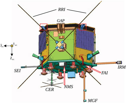
FIGURE 1. Spacecraft body-fixed frame of Swarm-E (on the left) and the e-POP instrument layout. RRI: Radio Receiver Instrument, GAP: GPS Attitude, Positioning, and Profiling experiment, SEI: Suprathermal Electron Imager, CER: Coherent Electromagnetic Radiation TOmography experiment, NMS: Neutral Mass and velocity Spectrometer, MGF: MaGnetic Field instrument, FAI: Fast Auroral Imager, IRM: Imaging and Rapid-Scanning Ion Mass Spectrometer.

2.2 Rotation matrices and transformation sequences

cavsiopy supports the transformations between GEI J2K/ICRF, ECEF, ITRF, NED, and NEC frames. The transformations between the frames are handled by applying appropriate rotations around x, y, and z axes in a particular order. The flowchart in Figure 2 displays the transformation sequences between the reference frames and corresponding rotation matrices that cavsiopy includes. The open forms and derivations of each transformation are given below the flowchart.

FIGURE 2

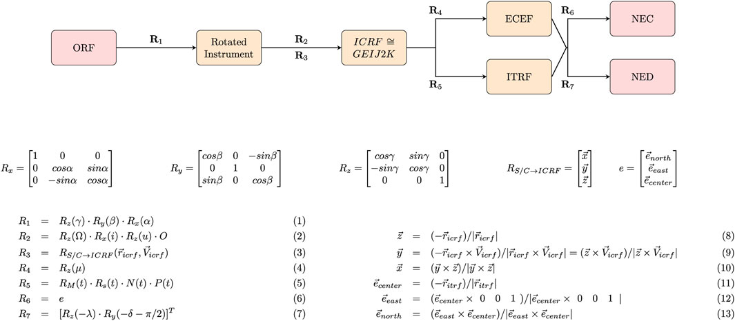
FIGURE 2. Flowchart for the transformations between the frames. The corresponding rotation matrices and the parameters are explicitly shown as follows. R_x, R_y, and R_z are the elementary rotation matrices; α: roll, β: pitch, and γ: yaw. R₁ (Eq. 1) is the direction cosine matrix to rotate the instrument frame. In R₂ (Eqn. 2), Ω is the right ascension of the ascending node; i, the satellite inclination; u, the argument of latitude (the sum of argument of perigee and the true anomaly); and O is a reordering matrix specific to a spacecraft. R₃ is formed using Eqns 8–10. In R₃ (Eqn. 3), r is the spacecraft position, and V is the velocity of the spacecraft in ICRF. In R₄ (Eqn. 4), μ is the azimuthal angle between the ICRF and ECEF frames. R₅ (Eqn. 5) is constructed via the multiplication of the precession (P(t)), nutation (N(t)), Earth rotation around the Conventional Ephemeris Pole (R_S), and polar motion (R_M) rotation matrices. In R₆, e is a vector representing the rotation from the terrestrial frames to the NEC frame, as shown in Eqns 11–13. λ is the spacecraft longitude, and δ is the spacecraft latitude in geodetic coordinates in R₇ (Eqn. 7).

In Figure 2 shows that R_x, R_y, and R_z are the elementary rotation matrices. R_x represents the rotation of the y–z plane about the x-axis by the roll angle (α). R_y depicts the rotation of the x–z plane about the y-axis by the pitch angle (β). Finally, R_z is the rotation of the x–y plane about the z-axis by the yaw angle (γ). For Swarm-E, the specific rotation sequence (R₁) to determine the instrument look direction in the spacecraft orbital reference frame (ORF) is in the order of roll, pitch, and yaw (RPY). The ordering may change for other spacecraft and is given as an optional input to cavsiopy routines. Additional rotations are required to transform the observation direction of the instrument in the ORF to a geodetic or geocentric coordinate system. The consecutive transformations from the ORF to reach the NED or NEC are as follows: to a celestial frame (GEI J2K/ICRF), then to a terrestrial frame, and finally to the geodetic/geocentric coordinate system. The terrestrial frame can be either ECEF or ITRF and can be transformed to NEC or NED coordinate systems using the appropriate rotation matrices, as shown in Figure 2.

R₂ and R₃ matrices are two approaches for the transformations between the ORF and GEI J2K/ICRF that are included as separate functions in cavsiopy. The star trackers on Swarm-E provide initial attitudes relative to the GEI J2K. In the present paper, GEI J2K and ICRF are treated as equal since the difference between the reference frames is in the order of 0.01 arcsec (Montenbruck and Gill, 2000; Book, 2019). For clarity, GEI J2K is sometimes referred to as the Mean Equator and Mean Equinox of J2000 (MEME J2K) or Earth-centered inertial frame J2000 (ECI J2K) in the literature. To compute R₂, knowledge of the orbital elements (right ascension of ascending node, inclination, and argument of latitude) and a reordering matrix (O) are needed (Capó-Lugo and Bainum, 2011; Canuto et al., 2018). cavsiopy utilizes the equations from Curtis (2014a) to compute the orbital elements for the R₂ transformation. The reordering matrix can be given to the corresponding cavsiopy function (orf_to_j2k_use_orbital_elements) as an optional input. Alternatively, R₃ can be derived from the position and velocity vectors of the spacecraft in GEI J2K/ICRF, as shown in Eqs 8–10 (Canuto et al., 2018).

The choice of the terrestrial reference frame for the third transformation depends on the required amount of accuracy. R₄ uses μ, which is the Greenwich Mean Sidereal Time (GMST) to rotate GEI J2K/ICRF into the more crude ECEF. GMST is the azimuthal angle between the ECEF and GEI J2K/ICRF and considers only the Earth’s rotation. cavsiopy follows Curtis (2014b) for the computation of GMST. R₄ does not account for the nutation, precession, and polar drift of the Earth. For higher accuracy, R₅ takes the precession (P(t)), nutation (N(t)), Earth rotation around the Conventional Ephemeris Pole (R_S), and polar motion (R_M) into account to transform to ITRF (Capitaine, 1990; Navipedia-ESA, 2014). cavsiopy determines R₅ using the C2T2000 subroutine of the Standards of Fundamental Astronomy (SOFA) library (Hohenkerk, 2011).

Finally, R₆ and R₇ are the rotation matrices used to obtain the instrument look direction in the NEC and NED coordinate systems, respectively. cavsiopy builds R₆ following Nielsen (2019) using the spacecraft position in the ITRF. To construct the NED rotation matrix R₇, spacecraft position in geodetic latitude and longitude is employed as in Cai et al. (2011).

For example, cavsiopy processes the rotation matrix multiplications in Eq. 1 to obtain an instrument’s look direction in the NED, using the ICRF and ITRF as intermediary frames.

$I_{\mathit{NED}}=R_7\cdot R_5\cdot R_3\cdot R_1\cdot I_{\mathit{ORF}}.(1)$

2.3 Limitations of the method

cavsiopy depends on the rotation matrices to determine the instrument look direction in the NEC and NED. The rotation matrices operate with sine and cosine functions, require sequential processing, and can lead to the occurrence of singularities. A major disadvantage of using rotation matrices is the gimbal lock that results when any of the two axes are aligned with each other at exact 90° rotations. In such cases, the degree of freedom decreases from three to two dimensions (Choe and Faraway, 2004). For Swarm-E, the yaw, pitch, and roll angles are derived from the attitude quaternions; thus, the gimbal lock issue is avoided. In addition, the users should be aware of the level of accuracy from the available attitude sensors and the temporal resolution of attitude solutions. Thus, the user should be mindful and take caution when there is a large amount of uncertainty in the attitude solutions. cavsiopy includes the plot_attitude_accuracy function to inspect the Swarm-E accuracy using the accuracy values in the RRI data files. The accuracy information of the Swarm-E can also be obtained from the Swarm-E quaternion files by using the import_quaternions function of the cavsiopy.

3 cavsiopy

cavsiopy takes the instrument body vector, spacecraft attitude (roll, pitch, and yaw angles), and spacecraft ephemeris as inputs. cavsiopy can be used to

1. determine the orientation of a spacecraft in the ORF;

2. determine the look direction of an instrument in the ORF;

3. find the look direction of an instrument onboard a spacecraft in any of the GEI J2K/ICRF, ECEF, ITRF, NED, and NEC;

4. calculate

• the look angles of the spacecraft (elevation and azimuth),

• the pointing angles of the instrument (elevation and azimuth),

• the distance between the spacecraft and a designated point on the ground, and

•the straight-line propagation (line-of-sight: LOS) vector from a specific point (target) to the spacecraft;

5. compute the rotation matrices for the transformations between ORF, GEI J2K/ICRF, ECEF, ITRF, NED, and NEC;

6. visualize the observation geometry, the trajectory of the spacecraft, and the instrument direction in 2D and 3D.

Moreover, cavsiopy includes functions to import Swarm-E ephemeris files and two-line-element (TLE) data from CelesTrak files to calculate the satellite orbital elements using spacecraft ephemeris and to compare the computed orbital elements with the imported TLE parameters.

3.1 Structure and components

cavsiopy comes with five modules: ephemeris_importer, use_rotation_matrices, attitude_analysis, attitude_plotter, and miscellaneous.

The ephemeris_importer module includes functions to read ephemeris in different formats from RRI data files (rri_ephemeris), ephemeris and spacecraft attitude from Swarm-E generic text files (cas_ephemeris), sp3 data files (sp3_ephemeris), and CelesTrak TLE files (import_tle). The compare_orbital function compares the computed orbital elements with the TLE provided values.

The attitude_analysis module utilizes the functions in the use_rotation_matrices module to find the direction of the instruments (find_instrument_attitude) as well as provide functions to calculate the closeness to slew for an instrument (find_slew_inst), the reception angles (calculate_reception_angle), the straight line propagation (line-of-sight) vector (calculate_los_vec), the pointing angles of the instrument (LA_inst), the look angles of the spacecraft (LA_sat), and the spacecraft distance from a designated point (spacecraft_distance_from_a_point).

The attitude_plotter module provides the visualization functionality of cavsiopy. The spacecraft trajectory, 2D and 3D view of the observation geometry, the time series of the closeness to slew, and the reception angles can be plotted by making use of the functions under the attitude_plotter. Example outputs from the plotting functions are detailed in Section 4. Moreover, the functions under the miscellaneous module can be used to mark the 2D–3D plots and to combine png figures horizontally and vertically.

The auxiliary folder includes the functions for the preliminary processing of the RRI data files. The voltage_reader function imports voltages from the RRI data file. The data points in the voltage arrays that are not a number (NaN) or that are exactly 0.0, which occur when the signal is lost during data relaying to the ground station, can be counted via the nan_counter. The plot_data_validity plots the percentage of valid data points that is calculated using the nan_counter. The calculate_aspect can be utilized to calculate the angle between the magnetic field at the spacecraft location and the LOS vector reaching the RRI.

Figure 3 shows the cavsiopy GitHub repository hierarchy (https://github.com/icebearcanada/cavsiopy) and the functions under the five modules.

FIGURE 3

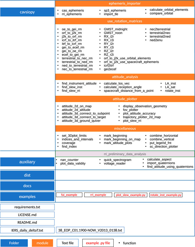
FIGURE 3. GitHub repository (https://github.com/icebearcanada/cavsiopy) hierarchy and the package contents.

3.2 Installation and dependencies

cavsiopy depends on h5py, geopy, astropy, pysofa2, numpy, matplotlib, and cartopy. pysofa2 is required for the transformations between the ICRF and ITRF to construct R₅. h5py is a requirement for astropy and is also employed for importing RRI hdf5 files, geopy is utilized to calculate the straight-line propagation vector and to find the distance between the spacecraft and the target location, astropy is used for the Julian date calculations, numpy is used for numerical calculations, and matplotlib and cartopy are used for the plotting tools.

cavsiopy can be directly downloaded from the associated GitHub repository or from Zenodo (Kalafatoglu Eyiguler et al., 2023b). Furthermore, installation is possible via the pip install cavsiopy command. The initial release (v1.0.0) needed to compile C shared libraries for pysofa (https://code.google.com/archive/p/pysofa/. Versions after v1.1.0 use the pysofa2 package (https://github.com/duncaneddy/pysofa2), which builds and distributes the shared C libraries during installation. Detailed instructions on how to install cavsiopy can be found on the cavsiopy GitHub repository and in the online documentation.

3.3 Documentation

The documentation covers the inputs and outputs to the modules and the functions that make up the cavsiopy modules. Each function in the modules has documentation strings (docstrings) right after the function declaration to provide detailed information about the inputs and outputs to the function and the methods and references used for computing the desired outputs. Online documentation can be accessed at https://cavsiopy.readthedocs.io/en/latest/.

4 Usage

Previously, Kalafatoglu Eyiguler et al. (2022); Kalafatoglu Eyiguler et al. (2023a); Kalafatoglu Eyiguler et al. (2023c); Pandey et al. (2022) employed cavsiopy modules to determine the angles that the incident radio wave makes with the RRI boresight and the dipole axes (reception angles) and to visualize the 3D geometry between the ground transmitter and the RRI onboard Swarm-E. Kalafatoglu Eyiguler et al. (2022); Kalafatoglu Eyiguler et al. (2023c) showed that the signal powers observed by a crossed-dipole antenna are significantly altered when reception angles are close to perpendicularity, at times, leading to complete loss of the signal. Kalafatoglu Eyiguler et al. (2023a) presented reception angle effects on the observed radio wave orientation angle at the RRI. The changes in the orientation angle of the radio wave from 180° to 0° (or vice versa) as expected from magnetoionic theory could not be resolved when the antenna boresight’s reception angle was approximately 90°. Pandey et al. (2022) analyzed a unique case of a single-mode radio wave traversing the ionosphere. The polarization properties of the single-mode radio wave were different when the antenna boresight was along the trajectory rather than pointing toward the target.

In the following section, illustrative examples and outputs from cavsiopy visualization tools are given for the RRI and the FAI onboard e-POP/Swarm-E to demonstrate the capabilities of cavsiopy. The example usage of the functions is provided under the example directory. rri_example.py imports an RRI data file, finds the RRI instrument direction in the NEC, and plots the result in 3D. rotate_inst_example.py demonstrates how to rotate the instrument pointing vector via the roll, pitch, and yaw angles given the spacecraft-specific rotation sequence. fai_example.py imports a spacecraft ephemeris file, calculates the look direction of the FAI for a Nadir experiment case, and plots the FOV of the FAI on the ground. plot_slew_example.py provides an example routine to determine and plot the time series of the reception angles and the closeness to slew.

4.1 Determining instrument attitude

Three steps are needed to determine instrument attitude using cavsiopy:

Listing 1. Calling sequence to determine the RRI direction.

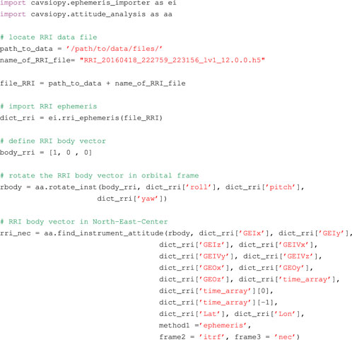
In cavsiopy, the default procedure to transform from the rotated antenna frame to the NEC is by using the rotation matrix derived from the spacecraft ephemeris (R₃), then performing the transformation to the ITRF, and finally to the NEC coordinate system. Other possible inputs for method1, frame2, and frame3 are orbital_elements, ecef, and ned, respectively.

In Listing 1, first the RRI body vector is specified. Then, ephemeris information is imported from the RRI data files before determining the RRI look direction. However, not all instrument data files contain ephemeris information. In that case, cas_ephemeris and sp3_ephemeris functions can be employed for Swarm-E:

Listing 2. Calling sequence to work with spacecraft ephemeris files.

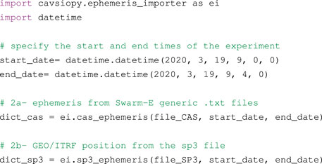
sp3 files contain the ITRF/GEO positions cavsiopy uses to calculate the ITRF-NEC rotation matrix (R₆). The sp3_ephemeris function works for all spacecraft since sp3 files contents and format are standard (Spofford and Remondi, 1994).

4.2 2D plotting functions

Figure 4 demonstrates example outputs from the 2D plotting functions in cavsiopy using the slew-to-target experiment carried out on 18 April 2016 reported in Danskin et al. (2018). The spacecraft trajectory is overlaid on the map in Figure 4A using the trajectory_plotter_2d_map function. Given the look direction of the instrument throughout the trajectory, attitude_2d_on_map plots the look direction vectors on top of the trajectory overlaid on the map, as shown in Figure 4B. For altitude plots, attitude_altitude_plots can be utilized to plot the spacecraft trajectory and the look directions in the longitude vs. altitude (Figure 4C) and latitude versus altitude grids (Figure 4D).

FIGURE 4

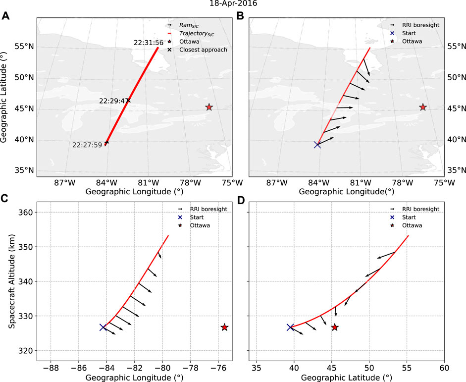
FIGURE 4. Two-dimensional plotting capabilities of cavsiopy: (A) spacecraft trajectory and the instrument pointing direction vectors (B) overlaid on the map, (C) longitude–altitude, and (D) latitude–altitude grid. In all plots, the red star denotes Ottawa location; the black vectors indicate the RRI boresight direction; the red solid line, the spacecraft trajectory; and the blue cross the beginning of the pass. The closest approach is located with the black cross in (A).

In all panels in Figure 4, the red, solid line shows the Swarm-E trajectory, the blue cross the beginning of the pass, the black vectors the RRI boresight direction, and the red star, Ottawa. Figure 4 clearly demonstrates that on 18 April 2016, Swarm-E was in the west of Ottawa in the ascending mode (traveling toward northeast from southwest). The RRI was slewing toward the Natural Resources Canada (NRCan) Ottawa transmitter latitude-, longitude-, and altitude-wise at all times during the experiment.

4.3 3D visualization

Additionally, cavsiopy includes routines to visualize the observation geometry in 3 dimensions (3D). There are four options to choose from: 1—display_observation_geometry: to display geometry for any kind of attitude (Figure 5A), 2—attitude_3d_connect_to_subpoint: to locate the sub-satellite point projected on the ground map, favorable when an instrument points along the ram direction (Figure 5B), 3—attitude_3d_connect_to_target: to connect the spacecraft position to the target position via a simple line, favorable when an instrument points downward, and 4—attitude_3d_ground_quiver: to display the look directions overlaid on the ground map and in 3D view (Figure 5D). The fourth option is generally the preferred plotting routine for slew-to-target passes of the RRI. All 3D functions are fully customizable in terms of vector lengths, colors, linewidths, and legends.

FIGURE 5

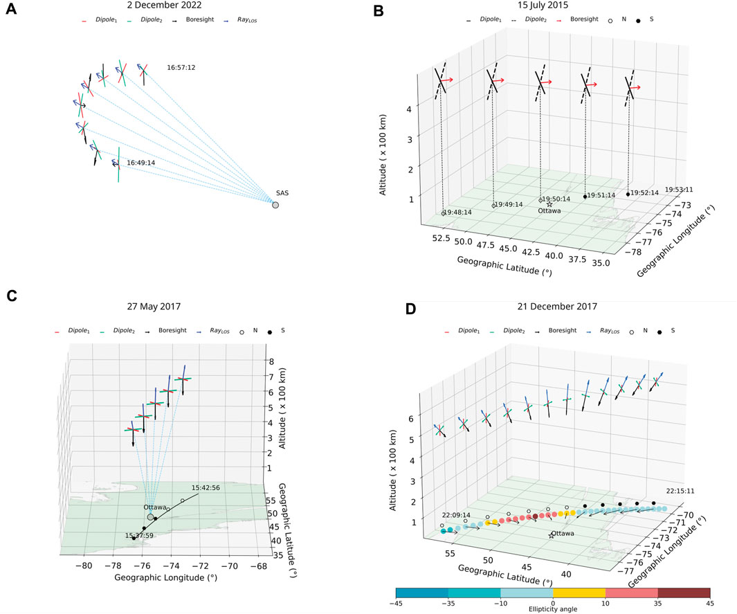
FIGURE 5. Three-dimensional plotting capabilities of cavsiopy: (A) 3D observation geometry; spacecraft location connected to the transmitting source; (B) spacecraft sub-satellite point projected onto the ground level; (C) spacecraft position connected to target; (D) a selected parameter scattered on the ground along with instrument look direction overlaid on the map.

Figure 5 illustrates the usage of the 3D plotting functions for the different attitude modes of the RRI. The RRI boresight and dipole attitudes are displayed in all panels. As shown in Figure 5A, the RRI is in a sun-pointing spinning attitude. Figure 5B shows the RRI in the ram mode, in which the RRI points along the spacecraft ram direction. The spacecraft location is projected onto the ground map. The hexagons indicate whether the spacecraft was to the north (filled with white) or to the south (filled with black) of the transmitter. As shown in Figure 5C, the RRI is looking downward, in RRI-nadir mode. Lastly, Figure 5D exemplifies a slew-to-target RRI experiment. The spacecraft location is connected to the target with blue dashed lines. Effective slew is implied if the RRI look direction (represented with black vectors) aligns with the dashed lines connecting the spacecraft to the target, which was the case around the middle of the pass in Figure 5C. In Figure 5D, the RRI look directions are shown with the black vectors overlaid on the ground map as well as the 3D pointing of the antenna. All vectors point toward the transmitter exhibiting slew. Furthermore, one of the key characteristics of the radio wave, the ellipticity angle, which describes the degree of the elliptical shape exhibited by the wave, is plotted as colored circles on the ground-projected trajectory as an additional parameter.

4.4 Determining and plotting slew using cavsiopy functions

In addition to determining and plotting the attitude of an instrument in 2D and 3D view, cavsiopy includes functions to quantify the closeness to slew for an instrument. To quantify the closeness to slew, the reception and complementary reception angles are defined. For the RRI, the reception angle is the angle between the RRI boresight’s look direction and the incident ray direction. If the reception angle (RA) of the boresight is 180°, RRI and the radio wave propagation path are aligned and the radio wave is incident on the front face of the antenna. If the RA is 0°, RRI receives the radio wave from its back face. Both conditions indicate slew-to-target passes and provide optimum measurement conditions. However, the rotation sense of the wave would be opposite between back and front face observations. Furthermore, when boresight RA is 90°, RRI would not able to fully detect the components of the radio wave.

The supplementary reception angle (SRA) of the RRI boresight and the complementary angles (CRAs) of the individual dipole axes show how far the RRI and each dipole are from the optimum slew condition, respectively. If the SRA is 0°, the RRI’s boresight is perfectly slewing toward the target. Similarly, if an individual dipole’s CRA is 0°, the dipole is in the optimum geometry to observe the radio wave.

For a crossed-dipole antenna, the observation capability for the radio wave polarization characteristics depends on the value of individual dipole CRAs and the boresight’s SRA. A receiving antenna onboard a spacecraft has a specific beamwidth within which optimum measurements are taken. For the RRI, the antenna beamwidth is considered to be 30°. Hence, if the incident radio wave direction and RRI boresight look direction are aligned within ±30°, the RRI is said to be effectively slewing toward the target, and observations would contain the optimum amount of information about the polarization characteristics of the radio wave.

In transionospheric radio wave studies, slew criteria may change according to the beamwidth of the receiving antenna being used. find_slew_rri and find_slew_inst functions in cavsiopy enable the test of the closeness to slew for multiple slew criteria. find_slew_rri is specialized for the RRI and takes the RRI boresight and dipole reception angles into account to determine the closeness to slew as in Listing 3. find_slew_inst considers only the pointing direction of the instrument and the beamwidth angle as input to the function.

Figure 6 showcases the SRA for the RRI boresight, CRAs for the individual dipoles, and the closeness to slew for different slew criteria for an RRI-Nadir pass on 27 May 2017. θ_SR denotes the boresight supplementary reception angle; ϕ_CD1 and ϕ_CD2 represent the dipole complementary reception angles.

During the 27 May experiment, the RRI front face was always looking downward; subsequently, θ_SR was always positive. The progression of CRA from negative to positive indicates that the spacecraft was approaching the target, made the closest approach, and then receded. CRAs at approximately 0° suggest that the dipoles and the RRI boresight attained favorable observation positions around the middle of the pass.

Figure 6 presents an RRI-Nadir experiment with the closeness to slew illustrated in the bottom panel. At the beginning and at the end of the pass, none of the slew criteria were met. However, in the middle of the pass, all slew criteria were met. Slew was possible within ±30° for more than 2 min between 15:39:20 and 15:41:30. The closeness to slew plot indicates that the best measurements of the radio wave characteristics (within ±5°) were possible around 15:40:10–15:40:20. The plot also provides the opportunity to interpret the evolution of the closeness to slew during a pass. Similar plots can be generated for any pass and instrument by following the slew_example.py.

Listing 3. Calling sequence for determining closeness to slew.

FIGURE 6

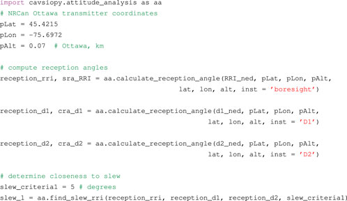
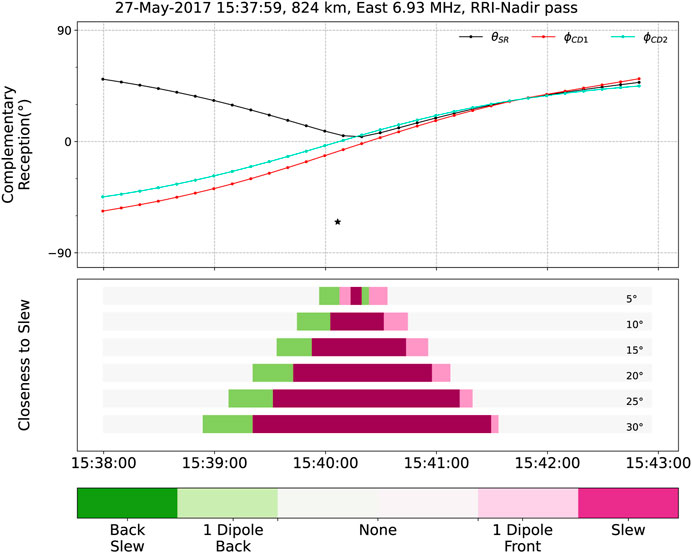
FIGURE 6. Complementary reception angles (top) and closeness to slew for multiple criteria (bottom). θ_SR is the boresight’s supplementary reception angle (black line), and the ϕ_CD1 (red line) and the ϕ_CD2 (cyan line) are the Dipole1 and the Dipole2 complementary reception angles, respectively. In the bottom panel, the dark green color shows that the radio wave was incident on the back face of the antenna, the light green color shows the radio wave was incident on the leading edges of the dipoles (90°–90° + slew criteria) within the slew limits to one dipole axis, the light pink color indicates the radio wave was incident to the end edges of the dipoles (90° ˗slew criteria) within the slew limits to one dipole axis, and lastly, the dark pink color represents the front face slew condition (both dipoles are in the optimum position for the observation). The white color denotes that the RRI was not in an optimum position to observe the radio wave components.

4.5 cavsiopy for other instruments

The IRM takes the best measurements when the spacecraft + x-axis is along the spacecraft ram direction and the IRM is pointing along the orbital frame −y-axis. Similar to the RRI, the IRM’s reception angle and slew can be determined to interpret the IRM measurements.

The Fast Auroral Imager can also be slewed to detect auroral structures. For example, Huyghebaert et al. (2021) used a set of experiments, in which the FAI was slewed toward the ICEBEAR E-region radar to investigate the coherent radar echoes in the presence of near-infrared auroral emissions.

The imager can only observe within their FOV. Relying solely on the reception angle is inadequate in determining the target area. An additional parameter, the projection of the FOV, is necessary for accurate mapping. cavsiopy provides a fov_plotter function to visualize an imager’s FOV. At present, the fov_plotter supports nadir-looking imager directions. Figure 7 depicts an FAI-nadir pass during an experiment with the ICEBEAR radar on 20 October 2020. The FAI look direction was directed downward and is represented by a black cross. The Swarm-E trajectory is illustrated by the red dashed line, while the location of the ICEBEAR radar site is marked by a pink star. The colored circles show the coverage area of the FAI observations.

FIGURE 7

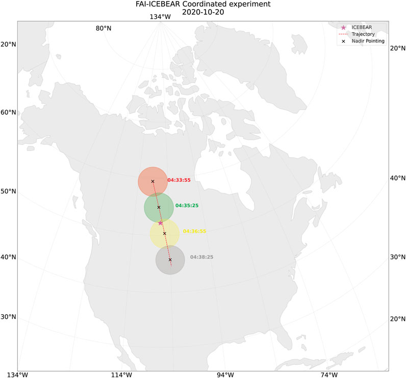
FIGURE 7. cavsiopy field of view of plot: The FAI look direction is shown with the black cross; the red dashed line and the pink star are the Swarm-E trajectory and the ICEBEAR radar site, respectively. The colored circles exhibit the coverage area of the FAI observations.

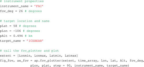
Listing 4 shows the procedure to plot the FOV of the FAI using the fov_plotter function of cavsiopy. ap is the abbreviation for the attitude_plotter module. By providing the spacecraft and target locations and the FOV angle of the imager (FOV_fai = 26°), the FOV of the instrument can be plotted on a geographical map projection.

Listing 4. Visualizing FAI field of view.

4.6 Auxiliary functions

The development efforts continue for the radio wave data analysis side of the project. The new routines to analyze RRI data are continually being developed, and previous routines are maintained according to the needs of the users. cavsiopy’s first release includes four functions (voltage_reader, quick_spectrogram, nan_counter, and plot_data_validity) for the preliminary analysis of the RRI data.

Figure 8 illustrates how the attitude information and the derived radio wave polarization characteristics can be blended together to form a combined interpretation of the features and the radio wave properties in the ionosphere.

voltage_reader imports the voltages from the RRI data files and prepares the data for further analysis. The general Stokes parameter approach is used to derive the secondary products from the induced complex voltages at the RRI. However, sometimes NaNs and zeroes in the voltage data arrays may affect the derived polarization characteristics. Thus, nan_counter ensures that the user is aware of the questionable data periods. plot_data_validity can be used to plot the information about the validity of data above the time axis in the form of a horizontal bar graph. quick_spectrogram plots the spectrogram of the complex voltages by considering the sampling rate (the default is 62.5 kHz). Other transmission sources and interference of other kind (instrument effects) can be inferred from a preliminary look at the spectrograms.

FIGURE 8

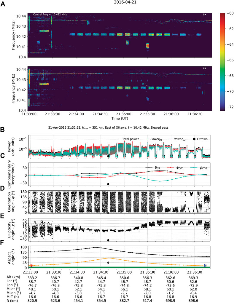
FIGURE 8. RRI complex voltage spectrograms (A), the calculated powers (B), the supplementary reception angle and complementary reception angles for the boresight and the dipoles (C), the derived polarization characteristics (D, E), the aspect and elevation angles, and the validity of observations (F). At the bottom of the plot are the spacecraft locations in the geographic altitude, latitude, longitude, magnetic latitude, magnetic longitude, magnetic local time (MLT), and the spacecraft distance from the target (R).

Apart from the data processing functions, three more functions are provided in the current auxiliary codes. calculate_aspect calculates the angle between the local magnetic field and the incident ray direction, called the aspect angle. The magnetoionic regime that the radio wave follows and the polarization characteristics that the radio wave would reflect are dependent on the aspect angle. Thus, knowledge of the aspect angle is crucial in the interpretation of the observed polarization characteristics. calculate_aspect utilizes the pyigrf package to calculate the local magnetic field. Hence, pyigrf is an additional dependency that should be installed beforehand for the users who would like to calculate the aspect angle using calculate_aspect.

The second function is import_quaternions, which processes the Swarm-E quaternion files and outputs the real and imaginary parts of the attitude quaternions, roll, pitch, and yaw angles and the attitude accuracy into a Python dictionary. import_quaternions depends on the spacepy to import the.cdf format files using the pycdf module. The function find_attitude_using_quaternions utilizes the imported attitude quaternions to determine the look direction of an instrument by factoring in the instrument’s body vector. The approach is based on the method described in Nielsen (2019) and works for all spacecraft in the Swarm constellation. Quaternions are computationally more efficient than the rotation matrix method. For Swarm-E in particular, quaternions are preferred for determining the instrument’s look direction since the corresponding files are readily available on the e-POP data server. However, quaternion files are not universally provided across all spacecraft missions. Alternatively, the roll, pitch, and yaw angles and the spacecraft ephemerides are disseminated. Regardless, both methodologies produce equivalent outcomes (Kalafatoglu Eyiguler et al., 2023c). The choice of the method is influenced by user preference and data availability.

Figure 8 provides a quick-look plot for the RRI complex voltage observations (Figure 8A), the calculated powers (Figure 8B), SRA of the boresight and the CRAs of the dipoles (Figure 8C), the derived polarization characteristics: the orientation angle (Figure 8D), the ellipticity angle (Figure 8E), the aspect and the elevation angle during the course of the experiment, and the validity of observations (Figure 8F).

The upper plot in panel A is the spectrogram of complex voltages at Dipole1 (D1), and the lower plot is the spectrogram of the complex voltages at Dipole2 (D2). The panel is a direct output of the quick_spectrogram function. The central frequency was 10.422 MHz during the experiment. The signal was received stronger at D1 than at D2. The spectrograms reveal that there were two interfering signals around 21:35:10 and 21:35:20.

The power at the dipoles (panel B), the orientation angle (panel D), and the ellipticity angle (panel E) were calculated using the Stokes module, which is not provided in cavsiopy since the derived parameters may not always represent the actual polarization state, and the interpretation requires careful consideration of the spacecraft attitude (Kalafatoglu Eyiguler et al., 2022; Kalafatoglu Eyiguler et al., 2023a; Kalafatoglu Eyiguler et al., 2023c). Stokes may be obtained separately as an auxiliary module by contacting the corresponding author.

The bar above the time axis in Figure 8 was plotted via the plot_data_validity function. The green color of the bar shows that the number of NaNs and zeroes in the data was sufficiently low such that the data can be considered valid throughout the experiment.

5 Summary

The present paper demonstrated the current capabilities of the cavsiopy Python package. cavsiopy is a light-weight, open-source, and easy-to-use instrument attitude determination package that does not require any a priori knowledge of the attitude determination methods, the quaternions, and the rotation matrices or the transformation sequences for usage. cavsiopy contains routines to determine the instrument attitude in the GEI J2K/ICRF, ECEF, and ITRF reference frames and the NED and NEC coordinate systems; to calculate the look angles of the spacecraft and the instruments onboard, the distance between a spacecraft and a designated point, and the line-of-sight vector from the point to the spacecraft; and to visualize the observation geometry in 2D and 3D. The transformation of the cavsiopy instrument attitude results to other representations of the geographic coordinate systems or to other reference frames (GSM, GSE, MAG, etc.) widely used by the heliospheric community can be accomplished via utilizing existing transformation routines provided by spacepy (Morley et al., 2010), pyspedas (Angelopoulos et al., 2019; Grimes et al., 2022), pysat (Stoneback et al., 2023), and astropy (Robitaille et al., 2013; Price-Whelan et al., 2022).

The maintenance of cavsiopy will be a collaborative effort between the University of Saskatchewan and the University of Calgary teams in the RRI working group. cavsiopy depends on scientific libraries astropy, cartopy, geopy, h5py, matplotlib, numpy, and pysofa2. A handicap may be the cavsiopy dependence on pysofa2 to compute the rotation matrix, R₅, for the ICRF to ITRF transformation. Since pysofa2 maintenance may not be simultaneous with cavsiopy maintenance, a smooth transition has been planned for computing R₅ within cavsiopy.

cavsiopy was specifically developed to complement the investigation and the interpretation of transionospheric radio waves using the RRI onboard e-POP/Swarm-E. The attitude of the receiving antenna plays an important role in the in situ reception and observation of signals. In a recent study by Kallio et al. (2022), a signal could only be detected in three of the fourteen experiments during the observation campaign. Kallio et al. (2022) listed the antenna pointing direction as one of the potential causes of the undetected radio waves during the coordinated experiments. Since the study lacked attitude and antenna pointing direction information, Kallio et al. (2022) could not conclude the specific reasons for the signal loss. In addition, the diagnostic tools for the ionosphere can only be employed after accounting for the reception angles of the antenna boresight and the dipoles (Kalafatoglu Eyiguler et al., 2023c). cavsiopy computes the observation geometry and the reception angle throughout a spacecraft’s trajectory to facilitate the interpretations of the observations made by the receivers onboard spacecraft.

5.1 Permission to reuse and copyright

Figures, tables, and images will be published under a Creative Commons CC-BY license, and permission must be obtained for use of copyrighted material from other sources (including re-published/adapted/modified/partial figures and images from the internet). It is the responsibility of the authors to acquire the licenses, to follow any citation instructions requested by third-party rights holders, and cover any supplementary charges.

Data availability statement

The datasets presented in this study can be found in online repositories. The names of the repository/repositories and accession number(s) can be found below: https://epop-data.phys.ucalgary.ca/.

Author contributions

ECKE: conceptualization, formal analysis, investigation, methodology, software, validation, visualization, writing–original draft, and writing–review and editing. WH: data curation, resources, software, validation, and writing–review and editing. ADH: data curation, resources, software, validation, and writing–review and editing. DWD: conceptualization, formal analysis, investigation, methodology, supervision, and writing–review and editing. KP: conceptualization, formal analysis, software, validation, and writing–review and editing. CJM: software and writing–review and editing. RGG: conceptualization and writing–review and editing. AWY: conceptualization, funding acquisition, project administration, resources, supervision, and writing–review and editing. GCH: conceptualization, funding acquisition, methodology, project administration, resources, supervision, and writing–review and editing.

Funding

The author(s) declare financial support was received for the research, authorship, and/or publication of this article. GCH and AWY acknowledge the financial support for this research from the Natural Sciences and Engineering Research Council (NSERC) Discovery Grants Program, under Grant #RGPIN-2019-19135 and RGPIN-2014-06069, respectively, and the CSA Grants and Contributions Program, under Grants #21SUSTTRRI, 16SUSTTPHF, and Grant #16SUSTSSPI, respectively.

Acknowledgments

The authors gratefully acknowledge the financial support from the Canadian Space Agency (CSA), MDA Corp., and the Industrial Technologies Office (ITO) for the development and the initial operations of the CASSIOPE satellite and the Enhanced Polar Outflow Probe (e-POP), and to the European Space Agency (ESA) Third-Party Mission (TPM) Programme for the continuing operations of CASSIOPE/e-POP as the fourth element of the Swarm Constellation (Swarm-E).

Conflict of interest

The authors declare that the research was conducted in the absence of any commercial or financial relationships that could be construed as a potential conflict of interest.

Publisher’s note

All claims expressed in this article are solely those of the authors and do not necessarily represent those of their affiliated organizations, or those of the publisher, the editors, and the reviewers. Any product that may be evaluated in this article, or claim that may be made by its manufacturer, is not guaranteed or endorsed by the publisher.

References

Acton, C., Bachman, N., Semenov, B., and Wright, E. (2018). A look towards the future in the handling of space science mission geometry. Planet. Space Sci. 150, 9–12. doi:10.1016/j.pss.2017.02.013

CrossRef Full Text | Google Scholar

Acton, C. H. (1996). Ancillary data services of nasa’s navigation and ancillary information facility. Planet. Space Sci. 44, 65–70. doi:10.1016/0032-0633(95)00107-7

CrossRef Full Text | Google Scholar

Angelopoulos, V., Cruce, P., Drozdov, A., Grimes, E., Hatzigeorgiu, N., King, D., et al. (2019). The space physics environment data analysis system (spedas). Space Sci. Rev. 215, 9–46. doi:10.1007/s11214-018-0576-4

PubMed Abstract | CrossRef Full Text | Google Scholar

Annex, A. M., Pearson, B., Seignovert, B., Carcich, B. T., Eichhorn, H., Mapel, J. A., et al. (2020). Spiceypy: a pythonic wrapper for the spice toolkit. J. Open Source Softw. 5, 2050. doi:10.21105/joss.02050

CrossRef Full Text | Google Scholar

Book, G. (2019).Navigation data—definitions and conventions Tech. rep CCSDS 500.0-G-4. Burlington, North Carolina, United States: The Consultative Committee for Space Data Systems.

Google Scholar

Cai, G., Chen, B. M., and Lee, T. H. (2011). “Advances in industrial control,” in Unmanned rotorcraft systems (Berlin, Germany: Springer International Publishing), 23–34.

CrossRef Full Text | Google Scholar

Canuto, E., Novara, C., Massotti, L., Carlucci, D., and Montenegro, C. P. (2018). “Chapter 11 - orbital control and prediction problems,” in Spacecraft dynamics and control. Editors E. Canuto, C. Novara, L. Massotti, D. Carlucci, and C. P. Montenegro (Oxford, United Kingdom: Butterworth-Heinemann), 565–606. doi:10.1016/B978-0-08-100700-6.00011-8

CrossRef Full Text | Google Scholar

Capitaine, N. (1990). The celestial pole coordinates. Celest. Mech. Dyn. Astronomy 48, 127–143. doi:10.1007/bf00049510

CrossRef Full Text | Google Scholar

Capó-Lugo, P. A., and Bainum, P. M. (2011). “4 - frame rotations and quaternions,” in Orbital mechanics and formation flying. Editors P. A. Capó-Lugo, and P. M. Bainum (Sawston, United Kingdom: Woodhead Publishing), 75–91. doi:10.1533/9780857093875.75

CrossRef Full Text | Google Scholar

Choe, S. B., and Faraway, J. J. (2004). Modeling head and hand orientation during motion using quaternions. SAE Trans. 113, 186–192.

CrossRef Full Text | Google Scholar

Crassidis, J. L. (2019). “Spacecraft attitude determination,” in Encyclopedia of systems and control. Editors J. Baillieul, and T. Samad (London, UK: Springer London), 1–7.

CrossRef Full Text | Google Scholar

Curtis, H. D. (2014a). Orbits in three dimensions. Third edn. Oxford, United Kingdom: Butterworth-Heinemann, 187–237. doi:10.1016/B978-0-08-097747-8.00004-9

CrossRef Full Text | Google Scholar

Curtis, H. D. (2014b). “Preliminary orbit determination,” in Orbital mechanics for engineering students. Third edn (Oxford, United Kingdom: Butterworth-Heinemann), 239–298. doi:10.1016/B978-0-08-097747-8.00005-0

CrossRef Full Text | Google Scholar

Danskin, D. W., Hussey, G. C., Gillies, R. G., James, H. G., Fairbairn, D. T., and Yau, A. W. (2018). Polarization characteristics inferred from the radio receiver instrument on the enhanced polar outflow probe. J. Geophys. Res. Space Phys. 123, 1648–1662. doi:10.1002/2017ja024731

CrossRef Full Text | Google Scholar

Grimes, E. W., Harter, B., Hatzigeorgiu, N., Drozdov, A., Lewis, J. W., Angelopoulos, V., et al. (2022). The space physics environment data analysis system in python. Front. Astronomy Space Sci. 9, 1020815. doi:10.3389/fspas.2022.1020815

CrossRef Full Text | Google Scholar

Heacock, R. L. (1980). The voyager spacecraft. Proc. Institution Mech. Eng. 194, 211–224. doi:10.1243/pime_proc_1980_194_026_02

CrossRef Full Text | Google Scholar

Hohenkerk, C. (2011). Standards of fundamental astronomy. Scholarpedia 6, 11404. doi:10.4249/scholarpedia.11404

CrossRef Full Text | Google Scholar

Huyghebaert, D., St.-Maurice, J.-P., McWilliams, K., Hussey, G., Howarth, A. D., Rutledge, P., et al. (2021). The properties of icebear e-region coherent radar echoes in the presence of near infrared auroral emissions, as measured by the swarm-e fast auroral imager. J. Geophys. Res. Space Phys. 126. doi:10.1029/2021ja029857

CrossRef Full Text | Google Scholar

James, H. G., Gillies, R. G., Hussey, G. C., and Prikryl, P. (2006). Hf fades caused by multiple wave fronts detected by a dipole antenna in the ionosphere. Radio Sci. 41. doi:10.1029/2005RS003385

CrossRef Full Text | Google Scholar

James, H. G. (2003). High-frequency direction finding in space. Rev. Sci. Instrum. 74, 3478–3486. doi:10.1063/1.1581396

CrossRef Full Text | Google Scholar

Kalafatoglu Eyiguler, E. C., Danskin, D. W., Howarth, A. D., Holley, W., Pandey, K., Gillies, R. G., et al. (May 2023a). Attitude effects on the observed orientation angle of hf waves from the radio receiver instrument on e-pop/swarm-e. In Proceedings of the ionospheric effects symposium 2023 (IES2023), Alexandria, Virginia.

Google Scholar

Kalafatoglu Eyiguler, E. C., Danskin, D., Hussey, G., Pandey, K., Gillies, R., and Yau, A. (May 2022). Satellite attitude effects on the reception of transionospheric hf signals: examples from the radio receiver instrument onboard e-pop/swarm-e. In Proceedings of the 2022 3rd URSI atlantic and asia pacific radio science meeting (AT-AP-RASC), Gran Canaria, Spain.

Google Scholar

Kalafatoglu Eyiguler, E. C., Holley, W., Howarth, A. D., Danskin, D. W., Pandey, K., Martin, C. J., et al. (2023b). icebearcanada/cavsiopy: v1.1.1. https://zenodo.org/record/8361257.

Google Scholar

Kalafatoglu Eyiguler, E. C., Pandey, K., Howarth, A., Holley, W., Danskin, D., Hussey, G., et al. (2023c). Effect of spacecraft attitude on radio wave polarization measurements for the radio receiver instrument on swarm-e. Adv. Space Res., doi:10.1016/j.asr.2023.09.001

CrossRef Full Text | Google Scholar

Kallio, E., Kero, A., Harri, A.-M., Kestilä, A., Aikio, A., Fontell, M., et al. (2022). Radar—cubesat transionospheric hf propagation observations: suomi 100 satellite and eiscat hf facility. Radio Sci. 57. doi:10.1029/2022rs007516

CrossRef Full Text | Google Scholar

Lee, A. Y., and Burk, T. A. (2019). Cassini spacecraft attitude control system performance and lessons learned, 1997–2017. J. Spacecr. Rockets 56, 158–170. doi:10.2514/1.a34236

CrossRef Full Text | Google Scholar

Montenbruck, O., and Gill, E. (2000). Satellite orbits, models, methods and applications. Berlin, Germany: Springer.

Google Scholar

Morley, S. K., Koller, J., Welling, D. T., Larsen, B. A., Henderson, M. G., and Niehof, J. T. (June 2010). Spacepy—a python-based library of tools for the space sciences. In Proceedings of the 9th Python in science conference (SciPy 2010) (Austin, TX, USA

Google Scholar

Navipedia-Esa, (2014). Transformation between celestial and terrestrial frames. https://gssc.esa.int/navipedia/index.php/transformation_between_Celestial_and_Terrestrial_Frames (Last accessed on June 21, 2023).

Google Scholar

Nielsen, J. B. (2019).Swarm level 1b processor algorithms (issue 6.11) Tech. rep. SW-RS-DSC-SY-0002. Paris, France: European Space Agency ESA.

Google Scholar

Pandey, K., Eyiguler, E. K., Gillies, R. G., Hussey, G. C., Danskin, D. W., and Yau, A. W. (2022). Polarization characteristics of a single mode radio wave traversing through the ionosphere: a unique observation from the rri on epop/swarm-e. J. Geophys. Res. Space Phys. 127. doi:10.1029/2022JA030684

CrossRef Full Text | Google Scholar

Price-Whelan, A. M., Lim, P. L., Earl, N., Starkman, N., Bradley, L., Shupe, D. L., et al. (2022). The astropy project: sustaining and growing a community-oriented open-source project and the latest major release (v5. 0) of the core package. Astrophysical J. 935, 167. doi:10.3847/1538-4357/ac7c74

CrossRef Full Text | Google Scholar

Robitaille, T. P., Tollerud, E. J., Greenfield, P., Droettboom, M., Bray, E., Aldcroft, T., et al. (2013). Astropy: a community python package for astronomy. Astronomy Astrophysics 558 (A33), A33. doi:10.1051/0004-6361/201322068

CrossRef Full Text | Google Scholar

Spofford, P. R., and Remondi, B. W. (1994). The national geodetic survey standard gps format sp3. https://files.igs.org/pub/data/format/sp3_docu.txt.

Google Scholar

Stoneback, R. A., Burrell, A. G., Klenzing, J., and Smith, J. (2023). The pysat ecosystem. Front. Astronomy Space Sci. 10. doi:10.3389/fspas.2023.1119775

CrossRef Full Text | Google Scholar

Yau, A. W., Howarth, A., White, A., Enno, G., and Amerl, P. (2015). Imaging and rapid-scanning ion mass spectrometer (irm) for the cassiope e-pop mission. Space Sci. Rev. 189, 41–63. doi:10.1007/s11214-015-0149-8

CrossRef Full Text | Google Scholar

Yau, A. W., and James, H. G. (2015). Cassiope enhanced polar outflow probe (e-pop) mission overview. Space Sci. Rev. 189, 3–14. doi:10.1007/s11214-015-0135-1

CrossRef Full Text | Google Scholar