Evaluating the performance of empirical models of total electron density and whistler-mode wave amplitude in the Earth’s inner magnetosphere

Empirical models have been previously developed using the large dataset of satellite observations to obtain the global distributions of total electron density and whistler-mode wave power, which are important in modeling radiation belt dynamics. In this paper, we apply the empirical models to construct the total electron density and the wave amplitudes of chorus and hiss, and compare them with the observations along Van Allen Probes orbits to evaluate the model performance. The empirical models are constructed using the Hp30 and SME (or SML) indices. The total electron density model provides an overall high correlation coefficient with observations, while large deviations are found in the dynamic regions near the plasmapause or in the plumes. The chorus wave model generally agrees with observations when the plasma trough region is correctly modeled and for modest wave amplitudes of 10–100 pT. The model overestimates the wave amplitude when the chorus is not observed or weak, and underestimates the wave amplitude when a large-amplitude chorus is observed. Similarly, the hiss wave model has good performance inside the plasmasphere when modest wave amplitudes are observed. However, when the modeled plasmapause location does not agree with the observation, the model misidentifies the chorus and hiss waves compared to observations, and large modeling errors occur. In addition, strong (>200 pT) hiss waves are observed in the plumes, which are difficult to capture using the empirical model due to their transient nature and relatively poor sampling statistics. We also evaluate four metrics for different empirical models parameterized by different indices. Among the tested models, the empirical model considering a plasmapause and controlled by Hp* (the maximum Hp30 during the previous 24 h) and SME* (the maximum SME during the previous 3 h) or Hp* and SML has the best performance with low errors and high correlation coefficients. Our study indicates that the empirical models are applicable for predicting density and whistler-mode waves with modest power, but large errors could occur, especially near the highly-dynamic plasmapause or in the plumes.

1 Introduction

The dynamic evolution of Earth’s outer radiation belt electron fluxes is strongly affected by whistler-mode waves and the cold electron density through the wave-particle interaction processes (Thorne et al., 2021). After the electrons are injected from the nightside plasma sheet, whistler-mode chorus waves scatter the energetic electrons at ∼1–100 keV energies, causing their fluxes to decay along the drift trajectory in the magnetosphere and precipitate them into the Earth’s upper atmosphere (Thorne et al., 2010; Tao et al., 2011; Ma et al., 2012). Following the commencement of geomagnetic storm and the subsequent substorms, chorus waves accelerate relativistic electrons at ∼100 s keV - 10 MeV energies to build up the Earth’s outer radiation belt (Reeves et al., 2013; Thorne et al., 2013; Li et al., 2016b; Ma et al., 2018). Hiss waves in the plasmasphere and plumes scatter the electrons at ∼10 keV–1 MeV energies, causing the radiation belt electron flux to decay during the storm recovery phase (Ni et al., 2013; Ma et al., 2016a). The energy-dependent slot region forms between the inner and outer radiation belts due to the dominant pitch angle scattering loss by hiss (Reeves et al., 2016; Ripoll et al., 2016; Zhao et al., 2019). The total electron density affects the electron resonance energy due to chorus and hiss waves and the efficiencies of pitch angle scattering and acceleration (Summers et al., 2007).

Whistler-mode chorus waves are commonly observed in the low-density plasma trough over the nightside-dawn-dayside magnetic local time (MLT) sectors (Li et al., 2009; Meredith et al., 2012; 2020; Agapitov et al., 2013). Chorus waves on the nightside are strong near the equator, and the waves on dayside have a broad latitudinal coverage with maximum power observed at off-equatorial latitudes (Agapitov et al., 2018). Chorus waves are generated by the unstable anisotropic hot electrons injected from the nightside plasma sheet (Li et al., 2008; Fu et al., 2014), with wave intensities closely related to electron injection events (Kasahara et al., 2009; Ma J. et al., 2022). The statistical wave power is well correlated with the auroral electrojet index of AE or AL, which indicates the strength of substorm injections. Chorus waves with high magnetic power are mainly observed to be quasi-parallel propagating. Another group of highly oblique chorus waves have high occurrence rates over the nightside-dawn sector close to the Earth (Li et al., 2016a).

Hiss waves are commonly observed in the high-density plasmasphere and plumes in the dayside and afternoon sectors (Summers et al., 2008; Li et al., 2015; Meredith et al., 2018; Kim and Shprits, 2019; Zhang et al., 2019). The major sources of hiss include the wave amplification by anisotropic electron distributions in the plumes or near the outer edge of the plasmasphere (Chen et al., 2012a; 2014; Li et al., 2013), the chorus waves propagating into the plasmasphere from the plasma trough (Bortnik et al., 2008; 2009; Meredith et al., 2021), and the lightning generated whistlers leaking from the ionosphere to the magnetosphere at low L shells (Sonwalkar and Inan, 1989; Bortnik et al., 2003; Meredith et al., 2006). The statistical wave power is stronger during more disturbed geomagnetic conditions (Kim et al., 2015; Spasojevic et al., 2015). The density structures in the outer plasmasphere or plumes modulate the hiss wave intensity (Malaspina et al., 2016; Li et al., 2019; Shi et al., 2019). In addition to the preferred wave amplification regions, the wave propagation could be focused, and enhanced in local high-density regions (Chen et al., 2012b).

Using multiple satellite mission data in the magnetosphere, previous statistical studies have revealed the global distribution of wave power and their dependence on geomagnetic activities. The empirical models are widely used to construct the global wave distributions and simulate the radiation belt electron evolution (Horne et al., 2013; Glauert et al., 2014; Drozdov et al., 2015; Ma et al., 2015). The radiation belt simulation using empirical wave models could produce a reasonable estimate of the electron flux decay and acceleration over a period longer than several days. However, event-specific wave distributions from in situ observations or other techniques are required to simulate the dynamic electron evolution in a short timescale or during high geomagnetic activities (Li et al., 2016b; Ma et al., 2018).

In this paper, we evaluate the performance of empirical models of total electron density and amplitudes of whistler-mode chorus and hiss waves in the Earth’s inner magnetosphere. Section 2 presents two events of total electron density and whistler-mode waves observed by Van Allen Probes. Section 3 presents the empirical model based on the statistics of the Van Allen Probes dataset, and the data distribution comparison between observation and modeling. Section 4 compares the performance of different models using error metrics and the Pearson correlation coefficient. Finally, in Section 5, we summarize and discuss our results.

2 Van Allen Probes observation of total electron density and whistler-mode waves

We use Van Allen Probes (RBSP) measurements (Mauk et al., 2013) to obtain the total electron density (N_e) and whistler-mode wave amplitudes (B_w) at L < 6.5 in the Earth’s inner magnetosphere. The Electric and Magnetic Field Instrument Suite and Integrated Science (EMFISIS) measures the DC magnetic fields and the AC signals of wave electric and magnetic fields over a broad frequency range (Kletzing et al., 2013). The background magnetic fields in three orthogonal directions are measured by the fluxgate magnetometer. The wave electric and magnetic power spectral densities at 10 Hz–12 kHz frequencies are measured by the Waveform Receiver (WFR), which also provides the wave polarization properties, including the wave normal angle, ellipticity, and planarity, calculated using the Singular Value Decomposition (SVD) method (Santolík et al., 2003). The High Frequency Receiver (HFR) measures the wave electric power spectral density from 10 kHz to 400 kHz, capturing the upper hybrid resonance band waves. The total electron density is calculated using the measured upper hybrid resonance frequency (Kurth et al., 2015). We also use the total electron density inferred using the spacecraft potential measured by the Electric Field and Waves (EFW) instrument (Wygant et al., 2013) when the upper hybrid resonance frequency is unavailable from HFR measurements. The density measurements from EFW have been calibrated against the more accurate EMFISIS density measurements (Breneman et al., 2022). We use the L shell from TS05 magnetic field model (Tsyganenko and Sitnov, 2005), provided by the ephemeris data products of Van Allen Probes.

In this section, we describe the total electron density and whistler-mode wave measurements during two events when Van Allen Probes apogees were at different MLTs. Then, we will compare modeling and observation during the two events in Section 3.3.

2.1 Observations on 01 March 2023

Figure 1 shows the total electron density and whistler-mode waves measured over a full day by Van Allen Probe A (panels C–F) and Probe B (panels G–J) on 01 March 2013. Figure 1A shows the geomagnetic Hp30 index (black) and Hp* values (blue). The Hp30 index is analogous to the Kp index but has a 30-min resolution (Matzka et al., 2022), and we define Hp* as the maximum Hp30 index during the previous 24 h. The 24 h timescale is chosen following the plasmapause models by Carpenter and Anderson (1992) and O'Brien and Moldwin (2003). Figure 1B shows the SuperMAG (Gjerloev, 2012) Auroral Electrojet index SML and the negative of SME*, where SME* is defined as the maximum SME index during the previous 3 h. The SML and SME indices are derived using SuperMAG magnetometer chains from more than 100 sites, and can more accurately indicate the substorm activity than auroral electrojet indices AL and AE (Newell and Gjerloev, 2011). A modest geomagnetic storm occurred on 01 March 2013, as analyzed by Ma et al. (2016b) and Bortnik et al. (2018). The maximum Hp30 index was close to 6, and the minimum SML index was about −1,400 nT, indicating a disturbed geomagnetic condition and particle injection activities.

FIGURE 1

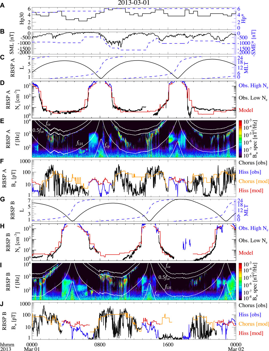
FIGURE 1. Van Allen Probes observation and empirical modeling of the total electron density and whistler-mode chorus and hiss waves on 01 March 2013. (A) Geomagnetic Hp30 index and Hp*, which is the maximum Hp30 index during the previous 24 h; (B) geomagnetic SML index and SME*, which is the maximum SME index in the previous 3 h; (C) L shell and MLT of Van Allen Probe A; (D) total electron densities observed by Van Allen Probe A in the high-density plasmasphere or plume (blue) and in the low-density plasma trough (black), and produced by the empirical model (red); (E) magnetic power spectrogram at 20 Hz–10 kHz frequencies observed by Van Allen Probe A, where the four white lines are equatorial electron gyrofrequency (f_ce), 0.5 f_ce, lower hybrid resonance frequency (f_LH), and proton gyrofrequency (f_cp); (F) chorus (black) and hiss (blue) wave amplitudes observed by Van Allen Probe A, and chorus (orange) and hiss (red) wave amplitudes produced from the empirical model. (G–J) Same as (C–F) except for the density and waves along the trajectory of Van Allen Probe (B).

The Van Allen Probes apogees were on the nightside (Figures 1C, G), suitable for measuring the whistler-mode chorus waves during this event. The measured total electron densities (Figures 1D, H) show a clear plasmapause structure with a large density gradient, the separation of the dense plasmasphere (blue) and tenuous plasma trough (black). Using the method described by Ma et al. (2021), we identified the high-density region (blue), including the plasmasphere and plumes, and the low-density region (black) of the plasma trough. We traced the density variations from perigee to apogee for each half orbit of the spacecraft. The region is first flagged as high-density from perigee. A low-density flag is triggered when a large value of negative density gradient is observed, and then a high-density flag is triggered when a large value of positive density gradient is observed. The densities inside identified high- and low-density regions are further compared to the empirical models to confirm the results. The detailed criteria are described by Ma et al. (2021) and not repeated here. The density data were averaged into a 1-min time cadence which is used in the statistical analysis in the following sections.

The wave magnetic power spectrograms (Figures 1E, I) show intense chorus waves at frequencies above (upper-band) and below (lower-band) 0.5 f_ce, where f_ce is the equatorial electron gyrofrequency. The chorus waves were observed over a wide range of MLTs on the nightside. The hiss waves at frequencies from ∼50 Hz to 1 kHz were observed mainly at L < 3.5 during this event, with weaker intensities compared to the chorus. We selected the whistler-mode wave intensities from the wave power spectrograms at frequencies from 20 Hz (or the equatorial proton gyrofrequency f_cp when f_cp > 20 Hz) to f_ce (or 10 kHz when f_ce > 10 kHz). In addition, we excluded the highly oblique magnetosonic waves by requiring that the wave ellipticity is greater than 0.5, the wave normal angle is below 80°, and the wave planarity is above 0.2. The chorus and hiss wave amplitudes were calculated in both the low-density and high-density regions, respectively, as shown by the black and blue lines in Figures 1F, J. During this event, the peak of chorus wave amplitude reached about 500 pT, and the hiss waves had weak amplitudes of tens of pT. We calculated the root-mean-square (RMS) wave amplitudes during each 1-min time cadence for statistical purposes.

2.2 Observations on 02 September 2013

Figure 2 shows the density and waves measurements made over a full day by Van Allen Probe A (panels C–F) and Probe B (panels G–J) on 02 September 2013. The maximum Hp30 index (Figure 2A) was 4, and the minimum SML index (Figure 2B) was about −900 nT, indicating a modestly disturbed geomagnetic condition.

FIGURE 2

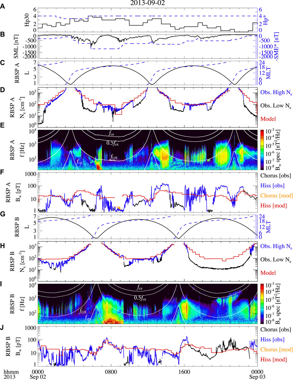
FIGURE 2. Same as Figure 1 except for the event on 02 September 2013.

The Van Allen Probes apogees were located on the dusk side (Figures 2C, G), which is suitable for measuring the plasmaspheric plumes and hiss waves during this event, as analyzed by Li et al. (2019). The measured total electron densities (Figures 2D, H) show evident density perturbations during each orbit of Van Allen Probes except for the Probe B observation after 16:00 UT. For example, during 13–21 UT, Figure 2D shows that Van Allen Probe A first traveled from the plasmasphere (blue) to the plasma trough (black), encountered plumes (blue) during 16:00–18:30 UT, and then traveled from the plasma trough (black) back to the plasmasphere (blue). The density measurements on different orbits suggest a highly dynamic variation of the plume on the dusk side.

Figures 2E, I show hiss wave activities with extended coverage in the high-density plasmasphere and plumes. The hiss waves at frequencies of ∼50 Hz–1 kHz are correlated with the high-density region, both during the extended plume period of 16:00–18:30 UT measured by Van Allen Probe A (Figures 2D, E) and for the short periods of density variations during 01–04 UT measured by Van Allen Probe B (Figures 2I, J). The magnetosonic waves were also observed below 50 Hz during 6–7 UT by Probe A (Figure 2E) and during 7–9 UT by Probe B (Figure 2I), but they were excluded from our wave data using the spectral criteria described above. The chorus waves were observed in the plasma trough during 19:00–22:30 UT by Probe B (Figure 2I). Figures 2F, J show that the peaks of hiss wave amplitudes (blue) are about 100 pT both in the plasmasphere and plumes.

3 Empirical model

3.1 Development of the empirical model

In previous studies, the surveys of whistler-mode chorus and hiss waves were usually modeled separately, and the full L-MLT distributions of both chorus and hiss waves were parameterized for different solar wind or geomagnetic conditions. However, the chorus and hiss waves are usually separated in space, with the chorus observed in the low-density plasma trough and the hiss observed in the high-density plasmasphere or plumes (e.g., Meredith et al., 2018; 2020). Therefore, an additional model of the plasmapause location or plasma density is required to construct the global distributions of chorus and hiss using the previous models.

We performed a survey using a unified dataset to analyze the total electron density, chorus wave amplitudes, and hiss wave amplitudes. This approach allowed us to construct consistent statistical distributions among them. Van Allen Probes measurements from September 2012 to October 2019 were used. To obtain the global distributions, we selected data when the magnetic latitude was within 10° from the magnetic equator. The survey of total electron density was performed at 2 < L < 6.5, considering that the density at L < 2 may not be reliable when the upper hybrid resonance frequency is higher than 500 kHz (Hartley et al., 2023). Surveys of chorus and hiss were performed at 1 < L < 6.5. The whistler-mode waves at L < 2 were identified as hiss throughout our survey. The data of average density and root-mean-square wave amplitudes were binned in every 1 h MLT and 0.5 L shell.

We used the combination of Hp* and SME* (or SML) indices to categorize the statistical distributions of the total electron density, chorus wave amplitude, and hiss wave amplitude. The plasmapause location in L-MLT was previously fitted as a function of the maximum Kp index in the previous 24–36 h by O'Brien and Moldwin (2003). The large amplitude chorus waves were generally found to be correlated with electron injections. The hiss waves are also related to the AE index, and were previously categorized by AE* by Li et al. (2015). Using the combination of Hp* and SME* or Hp* and SML, the model may better capture the plasmapause location and the wave activity. We set 7 levels of Hp* (Hp* ≤ 1, 1 < Hp* ≤ 2, 2 < Hp* ≤ 3, … Hp* > 6), and up to 4 levels of SME* (or SML) within each range of Hp*. The ranges of SME* (or SML) were set so that the data sample number is sufficient in each combination of Hp* and SME* (or SML), and the possible variation of SME* (or SML) is captured.

Using the Van Allen Probes dataset, we first obtained the occurrence rates of high-density (plasmasphere or plume) and low-density (plasma trough) flags in each L-MLT bin under each category of Hp* and SME*. Then, to construct a deterministic empirical model, we set the regions with a high-density occurrence rate higher than 0.5 to be the modeled plasmasphere or plume, and the regions with a low-density occurrence rate higher than 0.5 to be the modeled plasma trough.

The total electron densities with a high-density flag (blue) or a low-density flag (black) in Figures 1D, H, 2D, H were averaged in each L-MLT bin under each combination of Hp* and SME*. To construct the global density distribution, we used the average densities in the high-density region as the densities in the modeled plasmasphere or plume, and the average densities in the low-density region as the densities in the modeled plasma trough.

Similar to the density, we obtained the root-mean-square amplitudes of chorus and hiss waves in each L-MLT bin under each geomagnetic condition. To construct the global distributions for a certain geomagnetic condition, we assigned the chorus wave amplitudes in the modeled plasma trough, and hiss wave amplitudes in the modeled plasmasphere or plume. The modeled chorus and hiss waves are well separated in the space. Note that the chorus and hiss waves could be modeled using different parameters after the low- and high-density regions were modeled. For example, we first identified the high- and low-density flags using Hp* and SME* indices, and used Hp* and SML to model chorus in the high-density regions and Hp* and SME* to model hiss in the low-density regions. The model performances for different parameters are discussed in Section 4. The performance of the chorus wave amplitude model using Hp* and SML is found to be close to the performance of the model using Hp* and SME*.

3.2 Statistical distributions

Figure 3 shows the statistical distributions of the total electron density (panels A–D), chorus wave amplitude (panels E–H), and hiss wave amplitude (panels I–L) for the selected Hp*, SME*, and SML conditions. The sample numbers are shown in Figures 3M–T. The chorus waves are shown in the modeled plasma trough region, and hiss waves are shown in the modeled plasmasphere or plume. During quiet times (Figures 3A, E, I), the modeled plasmapause is mainly located at L > 6.5, and thus the densities mainly represent the plasmaspheric density, and the hiss waves are widely distributed at L < 6.5, consistent with an extended plasmasphere region. As geomagnetic conditions become more disturbed, the total electron densities are eroded over the nightside-dawn-dayside sectors, showing an MLT-dependent plasmapause. The high density in the dusk sector during the disturbed time (Figure 3D) includes the data samples of plumes or extended plasmasphere compared to other MLTs. The chorus wave power is enhanced over the nightside-dawn-dayside sectors as the geomagnetic activity becomes more disturbed (Figures 3F–H). Figures 3I–L show that the hiss wave powers are enhanced on the dayside and the dusk side at high L shells when Hp* and SME* increase, although the overall spatial coverage becomes more limited due to the erosion of the plasmapause. The statistical distributions of total electron density and whistler-mode waves are consistent with the previous survey results (e.g., Sheeley et al., 2001; Li et al., 2009; 2015; Meredith et al., 2018; 2020). Compared to the mean values, the standard deviation of total electron density is generally lower than the mean value, while the standard deviations of chorus and hiss wave amplitudes could be comparable or larger than the mean values (Supplementary Figure S1). Although the distributions under 4 conditions of Hp* and SME* (or SML) are shown in Figure 3, the empirical models cover all geomagnetic conditions and the full models are provided in the data repository.

FIGURE 3

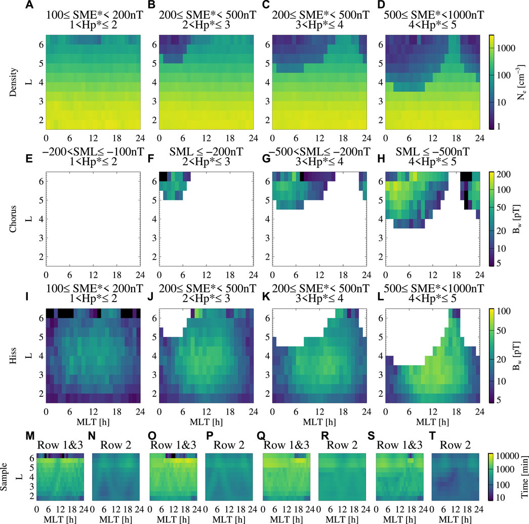
FIGURE 3. Statistical surveys of average total electron density (A–D), and root-mean-square amplitude of chorus (E–H) and hiss (I–L) as a function of MLT and L shell, categorized by different Hp* and SME* or Hp* and SML indices. (M) Total sample time under the geomagnetic condition for total electron density (Row 1, Panel A) or hiss (Row 3, Panel I), and (N) total sample time under the geomagnetic condition for chorus (Row 2, Panel E). (O–T) Same as (M,N) except for different geomagnetic conditions. (E–H) only show the data in the region where the low-density occurrence rate is higher than the high-density occurrence rate; (I–L) only show the data in the region where the high-density occurrence rate is higher.

3.3 Comparison between observation and modeling during the events

For a given value of Hp* and SME* (or SML) at a specific time, the empirical model provides the distribution of density and whistler-mode waves on a global scale by selecting data from the corresponding geomagnetic categories. The total electron density and whistler-mode wave amplitudes were modeled along the L shell and MLT of Van Allen Probes from September 2012 to October 2019. The modeled results were produced at 2 < L < 6.5 for the density and 1 < L < 6.5 for the wave amplitudes at a 1-min time cadence to compare with the observation. It is worth noting that the empirical model was developed using the data samples within 10° from the equator, while the Van Allen Probes measurements had additional sampling at latitudes up to 20°.

Figures 1D, F, H, J show the comparison between observation and modeling on 01 March 2013, when the Van Allen Probes apogees were on the nightside. The model (red) well captures the location of plasmapause and the density values in the plasmasphere and plasma trough (Figures 1D, H). The modeling was not performed during 16:30–19:00 UT on Van Allen Probe B (Figure 1H) because the L shell was larger than 6.5. The wave mode of chorus (orange) or hiss (red) is also correctly identified by the model (Figures 1F, J). Overall, the observations of chorus (black) and hiss (blue) show larger wave amplitude fluctuations than the modeling. The modeled chorus and hiss waves are persistently present in the low- and high-density regions, respectively, and may not reproduce the strong bursts or rapid disappearance of the observed waves. The large discrepancies are found at the peak of observed wave amplitude or when the whistler-mode waves were absent, i.e., at the extreme amplitudes. The modeling significantly overestimates the observed chorus waves during 15:00–16:30 UT observed by Probe B (Figure 1H), but the satellite was at high latitudes before traveling towards L ∼ 7, and the chorus waves were possibly damped in the nightside high-latitude region.

Figures 2D, F, H, J show the comparison on 02 September 2013 when the satellite apogees were on the dusk side. Plasmaspheric plumes were observed by Van Allen Probes (blue), which were not captured by the modeling. In Figure 2D, the modeling (red) shows the density structures of the plasmasphere and plasma trough during 04–12 UT, and only the plasmasphere during 13–21 UT. The modeling agrees with the observation when the high- and low-density regions are identified correctly.

Because the high- and low-density regions are potentially mis-identified by the model, the model predicts hiss waves when chorus waves are observed, and vice versa. The discrepancies in the wave amplitude modeling are larger than those in Figure 1 due to the mis-identification of the wave modes. For example, after 22:30 UT in Figure 2F, the observation shows that chorus B_w > 10 pT and hiss B_w = 0, and the modeling suggests that chorus B_w = 0 and hiss B_w > 10 pT. This causes an additional major source of modeling error, especially for the waves inside and near the plumes, in addition to the error sources found in Figure 1.

The two events in Figures 1, 2 are examples for the good model performance and for the potential issue in the empirical modeling, respectively, The plasmasphere was compressed to $L\lesssim 3$ during the event on 01 March 2013 (Figure 1), but the plasmapause structure was clear and the satellite did not observe plume structures. The modelled density agrees with the observation since the modeled plasmapause location was accurate. Plasmaspheric plumes were observed at the afternoon sector near the satellite apogee during the event on 02 September 2013 (Figure 2). Because the plasmaspheric plumes are highly dynamic and cause large density variations, they are less predictable using an empirical model which assumes a static state for a certain geomagnetic condition category. Machine learning technique may improve the performance for the electron densities during plasmaspheric plume activities.

3.4 Comparision of data distributions from observation and modeling

We compare the data distribution from observations and modeling using the ∼7-year dataset at 1-min time cadence. In this comparison and the evaluation of modeling performance discussed in Section 4, we only used the data when the Van Allen Probes were located within 10° from the equator. The entire dataset including all geomagnetic conditions is compared in Figure 4.

FIGURE 4

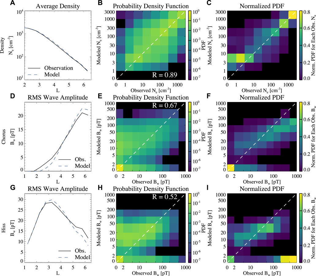
FIGURE 4. The comparison between observation and the empirical model, considering the Hp*, SME* index and modeled plasmapause for density and hiss, and considering the Hp*, SML index and modeled plasmapause for chorus. (A) The average density as a function of L, where the solid and dashed lines are observation and modeling results, respectively; (B) probability density distribution as a function of modeled and observed densities; (C) probability densities divided by the total probability density within each bin of observed density. (D–F) Same as (A–C) except for the chorus wave amplitude. (G–I) Same as (A–C) except for the hiss wave amplitude.

Figures 4A, D, G show the average total electron density, RMS amplitude of chorus, and RMS amplitude of hiss wave as a function of L. The observation generally agrees with the modeling results. The high- and low-density regions were modeled using a criterion of occurrence rate at 0.5 (see Section 3.1), causing the slight overestimate (underestimate) of chorus (hiss) B_w at L > 4.5, and slight underestimate (overestimate) of chorus (hiss) B_w at L < 4.5. If the average density and RMS B_w were weighted by the occurrence rates of high- and low-density regions in the models, the modeling would perfectly match the observation. However, such a model would not be very useful because it mixes the plasmasphere and plasma trough densities, and the modeled chorus and hiss waves appear simultaneously.

Figure 4B shows the probability density function (PDF) between the modeled and observed total electron densities. Most of the data are distributed around the diagonal line, suggesting a good model performance. The overall Pearson correlation coefficient (R) is 0.89. To examine the modeled data distribution for a fixed observation, Figure 4C shows the PDF divided by the sum of probability density in each range of observed N_e, denoted as the normalized PDF. The total normalized PDF for each range of observation is 1, so the good model will show a normalized PDF of ∼0.5–1 along the diagonal line. Figure 4C indicates good model performance when the observed density is higher than 100 cm^-3. The modeled data shows a wide spread for the observed densities from 10 cm⁻³ to 100 cm⁻³, suggesting a large deviation at and near the plasmapause or plumes. For the observed densities below 10 cm⁻³, the modeled density is mainly at 3–10 cm⁻³, suggesting that the model correctly identifies the low-density region of the plasma trough, but the modeled density is overall higher than the observation when the observed density is below 3 cm⁻³.

Figure 4E shows the probability density function for chorus waves. The modeled and observed chorus waves with 0 pT amplitude, including the high-density region data (chorus B_w = 0) in the modeling and observation, are included at B_w < 2 pT bins, and considered when evaluating the model performance. The high PDF at observed B_w < 2 pT and modeled B_w < 2 pT suggests that the majority of the plasmasphere regions are correctly modeled. A second group of data are found at observed B_w > 2 pT and modeled B_w < 2 pT, representing the times when the satellite was outside the plasmapause and observed chorus wave activity while the model suggests a high-density region. Similarly, the group of data at observed B_w < 2 pT and modeled B_w > 2 pT represents the times when the satellite was inside the plasmapause or chorus was not observed outside the plasmapause, while the model suggests a low-density region with chorus wave activity. Figure 4F shows the normalized PDF for each range of observed chorus B_w. The model underestimates the strong chorus wave amplitudes for observed B_w > 100 pT; specifically, the model most likely predicts a wave amplitude of 100–200 pT for the observed wave amplitude of 500–1,000 pT. The model provides a good estimate of the chorus wave amplitude for the observed chorus B_w from 10 pT to 100 pT. For the weak chorus waves with B_w < 10 pT, the model most likely overestimates the observation with modeled B_w of 10–20 pT. The overall Pearson correlation coefficient for chorus B_w is 0.67, which is lower than that of the density model. The correlation coefficient is affected by the groups of data at observed B_w > 2 pT and modeled B_w < 2 pT, and at observed B_w < 2 pT and modeled B_w > 2 pT; i.e., the R is strongly affected by the mis-identification of the plasmasphere or plasma trough.

Figure 4H shows the probability density function for hiss. The data distribution and scattering are similar to those of the chorus waves, while the amplitudes of observed and modeled hiss waves are overall lower than those of chorus. The group of data at observed B_w > 2 pT and modeled B_w < 2 pT represents the times when the spacecraft was in the high-density region and the model suggests a low-density region. The data group at observed B_w < 2 pT and modeled B_w > 2 pT represents the times when the spacecraft was in the low-density region or hiss was not observed, while the model suggests hiss wave activity in a high-density region. The normalized PDF distribution (Figure 4I) suggests that the modeling agrees with observation for observed B_w from 10 pT to 50 pT, underestimates for observed B_w > 50 pT, and overestimates for observed B_w < 10 pT. In addition, another evident group of data is found for observed B_w > 200 pT and modeled B_w < 2 pT in Figure 4I. The very large amplitude hiss waves, despite their overall low occurrence, are usually observed with large density variations or in the plumes (Shi et al., 2019). The empirical model may not fully capture the density variations, plume structures, or their evolution. Instead, these regions are likely mis-identified as the low-density plasma trough by the model, since the L shell of the perturbed density is usually high, and the geomagnetic condition is usually disturbed (Shi et al., 2019). As a result, the empirical model cannot capture the very large amplitude hiss waves. The Pearson correlation coefficient for hiss is 0.53, which is lower than that of chorus.

4 Performance of different models

4.1 Metrics for evaluating the model performance

We further evaluate the model performances using various error metrics and correlation coefficients for different L shells. In each L shell bin, we consider the data in the range ΔL = ±0.25. Following Morley et al. (2018), we consider Mean Absolute Error (MAE), Root Mean Square Error (RMSE), Median Symmetric Accuracy (MSA), and Pearson correlation coefficient. Below we define x as the observed N_e or B_w and y as the modeled N_e or B_w.

We calculate Mean Absolute Error normalized by the average of N_e or RMS of B_w as

$MAE/Mean=\overline{\left|y-x\right|}/\overline{x}\mathrm{f}\mathrm{o}\mathrm{r}{N}_{\mathrm{e}}(1)$

$MAE/RMS=\overline{\left|y-x\right|}/\sqrt{\overline{x^2}}\mathrm{f}\mathrm{o}\mathrm{r}{B}_{\mathrm{w}}(2)$

The Root Mean Square Error normalized by the average of N_e or RMS of B_w is calculated as

$RMSE/Mean=\sqrt{\overline{{\left(y-x\right)}^2}}/\overline{x}\mathrm{f}\mathrm{o}\mathrm{r}{N}_{\mathrm{e}}(3)$

$RMSE/RMS=\sqrt{\overline{{\left(y-x\right)}^2}}/\sqrt{\overline{x^2}}\mathrm{f}\mathrm{o}\mathrm{r}{B}_{\mathrm{w}}(4)$

The Median Symmetric Accuracy is calculated as

$MSA=100\left(e^{Median\left(\left|\ln \frac{y}{x}\right|\right)}|-|1\right)\mathrm{f}\mathrm{o}\mathrm{r}{N}_{\mathrm{e}}\mathrm{a}\mathrm{n}\mathrm{d}{B}_{\mathrm{w}}(5)$

The Pearson correlation coefficient is calculated as

$R=\frac{\sum \left(x-\overline{x}\right)\left(y-\overline{y}\right)}{\sqrt{\sum {\left(x-\overline{x}\right)}^2{\left(y-\overline{y}\right)}^2}}\mathrm{f}\mathrm{o}\mathrm{r}{N}_{\mathrm{e}}\mathrm{a}\mathrm{n}\mathrm{d}{B}_{\mathrm{w}}(6)$

All data, including the observed or modeled B_w = 0, are considered in Eqs 1–4, 6. To calculate MSA in Eq. 5, the logarithm function is used, so we consider all density data, and only the wave amplitude data with observed and modeled B_w > 10 pT. The good model is evaluated as having low MAE, low RMSE, low MSA, and high R.

Although the MSA cannot be calculated for B_w = 0, it provides a symmetric error for underestimate and overestimate in terms of the multiplication factor, while MAE and RMSE provide symmetric errors in terms of the percentage relative to the observation. For example, if $y=0.5x$, then $MAE=0.5$, $RMSE=0.5$, $MSA=100$; if $y=2x$, then $MAE=1$, $RMSE=1$, $MSA=100$ (same as for $y=0.5x$); if $y=1.5x$, then $MAE=0.5$ (same as for $y=0.5x$), $RMSE=0.5$ (same as for $y=0.5x$), $MSA=50$.

4.2 Comparing different models

We evaluate the performances of 6 models categorized by different combinations of Hp30 or Hp*, and SML or SME* indices, and the incorporation of the plasmapause. For each model, the surveys of total electron density, chorus wave amplitude, and hiss wave amplitude are performed using the same combination of geomagnetic indices. The statistical methods are the same as those described in Section 3 except for those described below. We perform the surveys of density and wave amplitudes using

• Empirical model 1: use Hp30 and SML indices, and consider the low- and high-density categorizations in the models (same as the density categorization method described in Section 3.1, and denoted as “PP”);

• Empirical model 2: use Hp30 index, and consider the low- and high-density categorizations;

• Empirical model 3: we perform the surveys of density and wave amplitudes using SML index, and consider the low- and high-density categorizations;

• Empirical model 4: use Hp* and SML indices, and consider the low- and high-density categorizations;

• Empirical model 5: use Hp* and SME* indices, and consider the low- and high-density categorizations;

• Empirical model 6: use Hp* and SME* indices; the low- and high-density categorization is not considered, but the model adopts the averages over both low- and high-density conditions weighted by their occurrence rates (denoted as “No PP”).

Models 1–3 only use the instantaneous geomagnetic conditions, and models 4–6 also consider the most disturbed Hp condition in the past 24 h. Model 6 is equivalent to the method of directly using the models of density, chorus, and hiss waves without imposing a plasmapause. The density and wave models are not coupled, the plasmaspheric density could be mixed with the plasma trough density, and the chorus and hiss wave could appear simultaneously in the same location. For Models 1–5, the empirical model of high- and low-density region is developed using the occurrence rates of high- and low-density flags for each individual model using the corresponding indices.

Figure 5 shows the metrics for different models as a function of the L shell. For the total electron density (Figures 5A–D), models 4 and 5 using Hp* have lower MAE, lower RMSE, lower MSA and higher R, than models 1, 2 and 3 using the Hp30 index. Although model 6 has a slightly lower RMSE and higher R than models 4 and 5, the MSA of model 6 is much higher than that of models 4 and 5. The best density model is model 5 using Hp*, SME*, and PP, with slightly lower errors and a higher correlation coefficient than model 4. Note that the R for the density data in each L shell bin is much lower than the overall R for all L shells (0.89 in Figure 4B). This is because the total electron density has a persistent L-dependence with high densities generally at low L shells, contributing to the high correlation coefficient when the data at different L shells are included in the R calculation.

FIGURE 5

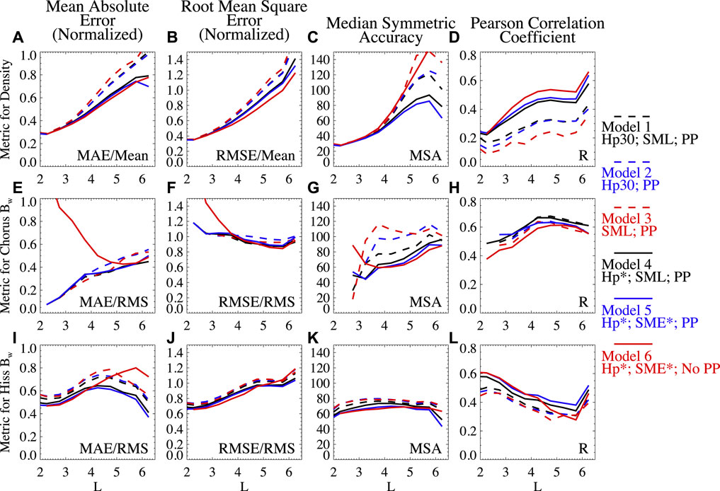
FIGURE 5. The performance of different empirical models evaluated using four metrics for different L shells. (A–D) Total electron density; (E–H) chorus wave amplitude; (I–L) hiss wave amplitude. The metrics include: Mean Absolute Error divided by the average of N_e or by the RMS B_w (chorus and hiss); Root Mean Square Error divided by the average of N_e or by the RMS B_w; Median Symmetric Accuracy; Pearson Correlation Coefficient R. The different empirical models are illustrated by different line styles or colors.

For the chorus B_w (Figures 5E–H), models 4 and 5 have slightly lower MAE and RMSE and slightly higher R at L < 4 than models 1, 2, and 3, and the improvement evaluated using MSA is significant. The different error trend for MSA compared to MAE or RMSE could be caused by the different penalization rules for underestimate and overestimate, different data samples used for error calculation (see Section 4.1), and non-Gaussian distribution of the data. Although model 6 shows the lowest RMSE and MSA at L > 3.5, it has the lowest R overall and significantly large MAE at L < 4. The best chorus wave models are 4 and 5 considering Hp*, SML (or SME*), and PP, and the R of model 4 is slightly higher than model 5.

For the hiss B_w (Figures 5I–L), models 4 and 5 have slightly lower RMSE and MSA than models 1, 2, and 3, and noticeable improvement evaluated using MAE and R. Compared to models 4 and 5, model 6 shows large MAE at L > 4 and low R at 4 < L < 6, and the performances at other regions or for other metrics are similar. The best model for hiss is model 5 considering Hp*, SME*, and PP, with higher R than model 4.

The performances between Model 4 and Model 5 are overall similar. We also performed a modeling using Hp* and SME indices and considering the low- and high-density categories (Supplementary Figure S2). Figure 5 shows slight improvement for modeling hiss B_w when SME* is considered compared to using SML, and the improvement for modeling chorus B_w is also shown by the model comparison between Model 5 and the model using Hp* and SME (Supplementary Figure S2).

The overall metrics for different models of density, chorus B_w and hiss B_w are also tabulated in Table 1, considering the data at all different L shells. Similar to the discussions above, the overall best model is model 4 for the density and hiss and model 5 for chorus, while their performance difference is very small. Significant modeling improvement is obtained using the Hp* index compared to the Hp30 index, and considering the low- and high-density categorization in the model.

TABLE 1

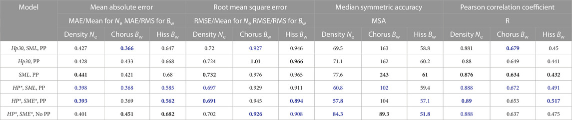
TABLE 1. The overall performance of different empirical models evaluated using four metrics. The best performance evaluated by each metric is highlighted in bold blue font; the second best is highlighted in blue font; the worst performance is highlighted in bold black font.

5 Conclusion and discussions

We evaluated the performance of a number of empirical models describing the total electron density and whistler-mode wave amplitudes in the Earth’s inner magnetosphere. The empirical models of density, chorus, and hiss waves were developed using the ∼7 years of Van Allen Probes data, categorized using Hp30, SME, SML indices, and their past maximum values, with a classification of high- or low-density regions (i.e., plasmasphere, plume or plasma trough). The models were used to reproduce the density and wave amplitudes along the Van Allen Probes trajectories, and the data distribution was compared between the observation and modeling results. We further used 4 metrics to compare the performances of 6 different models, categorized using different geomagnetic indices or excluding the density region classification. Our model performance evaluation indicates that:

• Incorporating the plasmapause (i.e., classifying the high- and low-density regions) significantly improves the modeling of total electron density as well as the amplitudes of chorus and hiss waves.

• Using the maximum values of geomagnetic indices during the past 3 h for SME and 24 h for Hp30 improves the modeling results compared to using only the instantaneous indices.

• The total electron density is well-modeled with high Pearson correlation coefficients using geomagnetic indices. The model agrees with the observation when the observed N_e > 3 cm^-3 and overestimates for smaller density observations. The additional errors are near the plasmapause or in the plumes, causing the large data spread in the probability density function distribution.

• The amplitudes of whistler-mode chorus and hiss waves are well-modeled when the observed wave amplitudes are moderate, with amplitudes between 10 and 100 pT. For the observed amplitude B_w < 10 pT or in the absence of whistler-mode waves, the chorus and hiss models tend to provide the average wave amplitudes, which overestimate the observation. The models underestimate the whistler-mode wave amplitudes when the observed amplitude is intense (>100 pT). The model cannot capture the very large amplitude (>200 pT) hiss waves, probably because these hiss waves are present in the plume region at high L shells during disturbed conditions, which is identified as the plasma trough by the model.

• The mis-identification of the plume region or the errors in identifying the plasmapause boundary causes large errors in modeling chorus and hiss wave amplitudes, because the chorus and hiss waves are mis-labeled by the model.

• To investigate the model performance properly, it is necessary to evaluate multiple error metrics and correlation coefficients. Using a single metric may provide a biased judgment for the model comparison.

Although we evaluated the performances of 6 different models, the chosen ‘best’ model is not yet optimized. For example, our model comparison mainly focused on the Hp30 and SME (or SML) indices and their derivatives, while the impacts of other geomagnetic indices and solar wind parameters have not been investigated. The solar wind dynamic pressure may significantly impact the whistler-mode waves at L > 6 due to the compression of the magnetosphere (Zhou et al., 2015; Yue et al., 2017). Following previous studies (O'Brien and Moldwin, 2003; Li et al., 2015), we incorporated the history of Hp30 and SME indices by simply using their maximum values in the past 24 h and 3 h, respectively. The history lengths of the indices are not tested, and the alternative method of using mean values of the indices is not investigated. The model optimization requires significant work efforts for an empirical model. However, the machine learning models inherently optimize the dependences of the model target on the parameters (Bortnik et al., 2016; Chu et al., 2017; 2021; Ma D. et al., 2022; Huang et al., 2022). The test of different empirical models could directly suggest the importance of each parameter, while the machine learning technique is more efficient in providing the best model fit for many parameters.

Our empirical models are developed using the Van Allen Probes data within 10° from the magnetic equator at L < 6.5. Additional data from the other spacecraft missions (THEMIS, Cluster, MMS, and Arase) provide the waves and density measurements at higher L shells or higher latitudes. In this paper, the comparison between Van Allen Probes data and the model results is limited to latitudes within ±10°. The chorus waves are confined close to the equator at the nightside, while the high powers of the dayside chorus are found at higher latitudes (Agapitov et al., 2018). A more comprehensive wave model in L shell, MLT, and magnetic latitude is required to properly capture the high-latitude wave power. The evaluation of the model performance in other regions is left as a future work.

Although the accuracy of the empirical models may be lower than the accuracy of machine learning models, the empirical model inherently provides the average density and wave power under a certain condition, which is stable and generally matches the data averaged over a sufficiently long period. The empirical model is robust if the data sampling time is sufficiently high in each category. The empirical models of total electron density and whistler-mode wave power are applicable to radiation belt modeling on a timescale longer than several days (Horne et al., 2013; Glauert et al., 2014; Drozdov et al., 2015), or under quiet to modestly disturbed geomagnetic conditions (Ma et al., 2015; 2017). During a short and disturbed period, the chorus and hiss wave amplitudes may be underestimated, or the plume regions may be misidentified. Therefore, the wave model based on observation (Li et al., 2016b; Ma et al., 2018) or from machine learning prediction (Bortnik et al., 2018) may provide better radiation belt modeling results. Our study of the empirical model performance provides a reference for the future development of machine learning models, by investigating the different error metrics and revealing the key factors affecting the model performance.

Data availability statement

The datasets presented in this study can be found in online repositories (https://doi.org/10.6084/m9.figshare.22762247). The names of the repository/repositories and accession number(s) can be found in the article/Supplementary Material.

Author contributions

QM performed the surveys using satellite data, constructed the empirical models, made model-data comparisons, evaluated the model performance, and wrote the manuscript. XC, DM, and SH performed machine learning modeling, which helped inspire the evaluation methods for the performance of the empirical models, discussed the strengths and weaknesses of the empirical model, and revised the manuscript. WL and JB discussed the results of this project, suggested improvements to the models, revised the manuscript, and provided support for this project. X-CS helped with the data preparation and global surveys, verified the data distribution, and revised the manuscript. All authors contributed to the article and approved the submitted version.

Funding

This work is supported by NASA grants 80NSSC19K0911, 80NSSC20K0196, and 80NSSC22K1023. In addition, we acknowledge NASA grants 80NSSC19K0845 and 80NSSC20K0698, 80NSSC20K0704 and the NSF grants AGS-1847818 and AGS-2225445. SH gratefully acknowledges the NASA FINESST grant 80NSSC21K1385. JB acknowledges support from the Defense Advanced Research Projects Agency under the Department of the Interior award D19AC00009.

Acknowledgments

We are grateful to the NASA and NSF agencies for their support of our research. The details of each grant are listed in the “Funding” section above. We acknowledge the efforts by Geospace Environment Modeling focus group Self-Consistent Inner Magnetospheric Modeling. We also acknowledge the Van Allen Probes teams for providing the data.

Conflict of interest

The authors declare that the research was conducted in the absence of any commercial or financial relationships that could be construed as a potential conflict of interest.

Publisher’s note

All claims expressed in this article are solely those of the authors and do not necessarily represent those of their affiliated organizations, or those of the publisher, the editors and the reviewers. Any product that may be evaluated in this article, or claim that may be made by its manufacturer, is not guaranteed or endorsed by the publisher.

Supplementary material

The Supplementary Material for this article can be found online at: https://www.frontiersin.org/articles/10.3389/fspas.2023.1232702/full#supplementary-material

References

Agapitov, O., Artemyev, A., Krasnoselskikh, V., Khotyaintsev, Y. V., Mourenas, D., Breuillard, H., et al. (2013). Statistics of whistler-mode waves in the outer radiation belt: cluster STAFF-SA measurements. J. Geophys. Res. Space Phys. 118, 3407–3420. doi:10.1002/jgra.50312

CrossRef Full Text | Google Scholar

Agapitov, O. V., Mourenas, D., Artemyev, A. V., Mozer, F. S., Hospodarsky, G., Bonnell, J., et al. (2018). Synthetic empirical chorus wave model from combined Van Allen Probes and Cluster statistics. J. Geophys. Res. Space Phys. 123, 297–314. doi:10.1002/2017JA024843

CrossRef Full Text | Google Scholar

Bortnik, J., Chu, X., Ma, Q., Li, W., Zhang, X., Thorne, R. M., et al. (2018). “Artificial neural networks for determining magnetospheric conditions,” in Machine learning techniques for space weather (Elsevier), 279–300. doi:10.1016/b978-0-12-811788-0.00011-1

CrossRef Full Text | Google Scholar

Bortnik, J., Inan, U. S., and Bell, T. F. (2003). Frequency-time spectra of magnetospherically reflecting whistlers in the plasmasphere. J. Geophys. Res. 108 (A1), 1030. doi:10.1029/2002JA009387

CrossRef Full Text | Google Scholar

Bortnik, J., Li, W., Thorne, R. M., and Angelopoulos, V. (2016). A unified approach to inner magnetospheric state prediction. J. Geophys. Res. Space Phys. 121 (3), 2423–2430. doi:10.1002/2015ja021733

CrossRef Full Text | Google Scholar

Bortnik, J., Li, W., Thorne, R. M., Angelopoulos, V., Cully, C., Bonnell, J., et al. (2009). An observation linking the origin of plasmaspheric hiss to discrete chorus emissions. Science 324 (5928), 775–778. doi:10.1126/science.1171273

PubMed Abstract | CrossRef Full Text | Google Scholar

Bortnik, J., Thorne, R. M., and Meredith, N. P. (2008). The unexpected origin of plasmaspheric hiss from discrete chorus emissions. Nature 452, 62–66. doi:10.1038/nature06741

PubMed Abstract | CrossRef Full Text | Google Scholar

Breneman, A. W., Wygant, J. R., Tian, S., Cattell, C. A., Thaller, S. A., Goetz, K., et al. (2022). The van allen Probes electric field and waves instrument: science results, measurements, and access to data. Space Sci. Rev. 218, 69. doi:10.1007/s11214-022-00934-y

CrossRef Full Text | Google Scholar

Carpenter, D. L., and Anderson, R. R. (1992). An ISEE/whistler model of equatorial electron density in the magnetosphere. J. Geophys. Res. 97, 1097–1108. doi:10.1029/91ja01548

CrossRef Full Text | Google Scholar

Chen, L., Li, W., Bortnik, J., and Thorne, R. M. (2012a). Amplification of whistler-mode hiss inside the plasmasphere. Geophys. Res. Lett. 39, L08111. doi:10.1029/2012GL051488

CrossRef Full Text | Google Scholar

Chen, L., Thorne, R. M., Bortnik, J., Li, W., Horne, R. B., Reeves, G. D., et al. (2014). Generation of unusually low frequency plasmaspheric hiss. Geophys. Res. Lett. 41, 5702–5709. doi:10.1002/2014GL060628

CrossRef Full Text | Google Scholar

Chen, L., Thorne, R. M., Li, W., Bortnik, J., Turner, D., and Angelopoulos, V. (2012b). Modulation of plasmaspheric hiss intensity by thermal plasma density structure. Geophys. Res. Lett. 39, L14103. doi:10.1029/2012GL052308

CrossRef Full Text | Google Scholar

Chu, X., Bortnik, J., Li, W., Ma, Q., Denton, R., Yue, C., et al. (2017). A neural network model of three-dimensional dynamic electron density in the inner magnetosphere. J. Geophys. Res. Space Phys. 122 (9), 9183–9197. doi:10.1002/2017ja024464

CrossRef Full Text | Google Scholar

Chu, X., Ma, D., Bortnik, J., Tobiska, W. K., Cruz, A., Bouwer, S. D., et al. (2021). Relativistic electron model in the outer radiation belt using a neural network approach. Space weather. 19, e2021SW002808. doi:10.1029/2021SW002808

CrossRef Full Text | Google Scholar

Drozdov, A. Y., Shprits, Y. Y., Orlova, K. G., Kellerman, A. C., Subbotin, D. A., Baker, D. N., et al. (2015). Energetic, relativistic, and ultrarelativistic electrons: comparison of long-term VERB code simulations with van allen Probes measurements. J. Geophys. Res. Space Phys. 120, 3574–3587. doi:10.1002/2014JA020637

CrossRef Full Text | Google Scholar

Fu, X., Cowee, M. M., Friedel, R. H., Funsten, H. O., Gary, S. P., Hospodarsky, G. B., et al. (2014). Whistler anisotropy instabilities as the source of banded chorus: van Allen Probes observations and particle-in-cell simulations. J. Geophys. Res. Space Phys. 119, 8288–8298. doi:10.1002/2014JA020364

PubMed Abstract | CrossRef Full Text | Google Scholar

Gjerloev, J. W. (2012). The SuperMAG data processing technique. J. Geophys. Res. 117, A09213. doi:10.1029/2012JA017683

CrossRef Full Text | Google Scholar

Glauert, S. A., Horne, R. B., and Meredith, N. P. (2014). Three-dimensional electron radiation belt simulations using the BAS Radiation Belt Model with new diffusion models for chorus, plasmaspheric hiss, and lightning-generated whistlers. J. Geophys. Res. Space Phys. 119, 268–289. doi:10.1002/2013JA019281

CrossRef Full Text | Google Scholar

Hartley, D. P., Cunningham, G. S., Ripoll, J.-F., Malaspina, D. M., Kasahara, Y., Miyoshi, Y., et al. (2023). Using Van Allen Probes and Arase observations to develop an empirical plasma density model in the inner zone. J. Geophys. Res. Space Phys. 128, e2022JA031012. doi:10.1029/2022ja031012

CrossRef Full Text | Google Scholar

Horne, R. B., Glauert, S. A., Meredith, N. P., Boscher, D., Maget, V., Heynderickx, D., et al. (2013). Space weather impacts on satellites and forecasting the Earth's electron radiation belts with SPACECAST. Space weather. 11, 169–186. doi:10.1002/swe.20023

CrossRef Full Text | Google Scholar

Huang, S., Li, W., Shen, X.-C., Ma, Q., Chu, X., Ma, D., et al. (2022). Application of recurrent neural network to modeling Earth's global electron density. J. Geophys. Res. Space Phys. 127, e2022JA030695. doi:10.1029/2022JA030695

CrossRef Full Text | Google Scholar

Kasahara, Y., Miyoshi, Y., Omura, Y., Verkhoglyadova, O. P., Nagano, I., Kimura, I., et al. (2009). Simultaneous satellite observations of VLF chorus, hot and relativistic electrons in a magnetic storm “recovery” phase. Geophys. Res. Lett. 36, L01106. doi:10.1029/2008GL036454

CrossRef Full Text | Google Scholar

Kim, K., Lee, D., and Shprits, Y. (2015). Dependence of plasmaspheric hiss on solar wind parameters and geomagnetic activity and modeling of its global distribution. J. Geophys. Res. Space Phys. 120, 1153–1167. doi:10.1002/2014JA020687

CrossRef Full Text | Google Scholar

Kim, K.-C., and Shprits, Y. (2019). Statistical analysis of hiss waves in plasmaspheric plumes using Van Allen Probe observations. J. Geophys. Res. Space Phys. 124, 1904–1915. doi:10.1029/2018JA026458

CrossRef Full Text | Google Scholar

Kletzing, C. A., Kurth, W. S., Acuna, M., MacDowall, R. J., Torbert, R. B., Averkamp, T., et al. (2013). The electric and magnetic field instrument suite and integrated science (EMFISIS) on RBSP. Space Sci. Rev. 179, 127–181. doi:10.1007/s11214-013-9993-6

CrossRef Full Text | Google Scholar

Kurth, W. S., De Pascuale, S., Faden, J. B., Kletzing, C. A., Hospodarsky, G. B., Thaller, S., et al. (2015). Electron densities inferred from plasma wave spectra obtained by the Waves instrument on Van Allen Probes. J. Geophys. Res. Space Phys. 120, 904–914. doi:10.1002/2014JA020857

PubMed Abstract | CrossRef Full Text | Google Scholar

Li, W., Ma, Q., Thorne, R. M., Bortnik, J., Kletzing, C. A., Kurth, W. S., et al. (2015). Statistical properties of plasmaspheric hiss derived from Van Allen Probes data and their Effects on radiation belt electron dynamics. J. Geophys. Res. Space Phys. 120, 3393–3405. doi:10.1002/2015JA021048

CrossRef Full Text | Google Scholar

Li, W., Ma, Q., Thorne, R. M., Bortnik, J., Zhang, X., Li, J., et al. (2016b). Radiation belt electron acceleration during the 17 March 2015 geomagnetic storm: observations and simulations. J. Geophys. Res. Space Phys. 121, 5520–5536. doi:10.1002/2016JA022400

CrossRef Full Text | Google Scholar

Li, W., Santolik, O., Bortnik, J., Thorne, R. M., Kletzing, C. A., Kurth, W. S., et al. (2016a). New chorus wave properties near the equator from Van Allen Probes wave observations. Geophys. Res. Lett. 43, 4725–4735. doi:10.1002/2016GL068780

CrossRef Full Text | Google Scholar

Li, W., Shen, X.-C., Ma, Q., Capannolo, L., Shi, R., Redmon, R. J., et al. (2019). Quantification of energetic electron precipitation driven by plume whistler mode waves, plasmaspheric hiss, and exohiss. Geophys. Res. Lett. 46, 3615–3624. doi:10.1029/2019GL082095

CrossRef Full Text | Google Scholar

Li, W., Thorne, R. M., Angelopoulos, V., Bortnik, J., Cully, C. M., Ni, B., et al. (2009). Global distribution of whistler-mode chorus waves observed on the THEMIS spacecraft. Geophys. Res. Lett. 36, L09104. doi:10.1029/2009GL037595

CrossRef Full Text | Google Scholar

Li, W., Thorne, R. M., Bortnik, J., Reeves, G. D., Kletzing, C. A., Kurth, W. S., et al. (2013). An unusual enhancement of low-frequency plasmaspheric hiss in the outer plasmasphere associated with substorm-injected electrons. Geophys. Res. Lett. 40, 3798–3803. doi:10.1002/grl.50787

CrossRef Full Text | Google Scholar

Li, W., Thorne, R. M., Meredith, N. P., Horne, R. B., Bortnik, J., Shprits, Y. Y., et al. (2008). Evaluation of whistler mode chorus amplification during an injection event observed on CRRES. J. Geophys. Res. 113, A09210. doi:10.1029/2008JA013129

CrossRef Full Text | Google Scholar

Ma, D., Chu, X., Bortnik, J., Claudepierre, S. G., Tobiska, W. K., Cruz, A., et al. (2022a). Modeling the dynamic variability of sub-relativistic outer radiation belt electron fluxes using machine learning. Space weather. 20, e2022SW003079. Available at: https://doi-org.colorado.idm.oclc.org/10.1029/2022SW003079.

CrossRef Full Text | Google Scholar

Ma, J., Gao, X., Chen, H., Tsurutani, B. T., Ke, Y., Chen, R., et al. (2022b). The effects of substorm injection of energetic electrons and enhanced solar wind ram pressure on whistler-mode chorus waves: A statistical study. J. Geophys. Res. Space Phys. 127, e2022JA030502. doi:10.1029/2022JA030502

CrossRef Full Text | Google Scholar

Ma, Q., Li, W., Bortnik, J., Thorne, R. M., Chu, X., Ozeke, L. G., et al. (2018). Quantitative evaluation of radial diffusion and local acceleration processes during GEM challenge events. J. Geophys. Res. Space Phys. 123, 1938–1952. doi:10.1002/2017JA025114

CrossRef Full Text | Google Scholar

Ma, Q., Li, W., Thorne, R. M., Bortnik, J., Reeves, G. D., Kletzing, C. A., et al. (2016a). Association between glycated hemoglobin A1c levels with age and gender in Chinese adults with no prior diagnosis of diabetes mellitus. J. Geophys. Res. Space Phys. 121 (11), 737–740. doi:10.3892/br.2016.643

PubMed Abstract | CrossRef Full Text | Google Scholar

Ma, Q., Li, W., Thorne, R. M., Bortnik, J., Reeves, G. D., Spence, H. E., et al. (2017). Diffusive transport of several hundred keV electrons in the Earth's slot region. J. Geophys. Res. Space Phys. 122 (10), 235–310. doi:10.1002/2017JA024452

CrossRef Full Text | Google Scholar

Ma, Q., Li, W., Thorne, R. M., Ni, B., Kletzing, C. A., Kurth, W. S., et al. (2015). Modeling inward diffusion and slow decay of energetic electrons in the Earth's outer radiation belt. Geophys. Res. Lett. 42, 987–995. doi:10.1002/2014GL062977

CrossRef Full Text | Google Scholar

Ma, Q., Li, W., Thorne, R. M., Nishimura, Y., Zhang, X., Reeves, G. D., et al. (2016b). Simulation of energy-dependent electron diffusion processes in the Earth's outer radiation belt. J. Geophys. Res. Space Phys. 121, 4217–4231. doi:10.1002/2016JA022507

CrossRef Full Text | Google Scholar

Ma, Q., Li, W., Zhang, X. -J., Bortnik, J., Shen, X. -C., Connor, H. K., et al. (2021). Global survey of electron precipitation due to hiss waves in the Earth's plasmasphere and plumes. J. Geophys. Res. Space Phys. 126, e2021JA029644. doi:10.1029/2021JA029644

CrossRef Full Text | Google Scholar

Ma, Q., Ni, B., Tao, X., and Thorne, R. M. (2012). Evolution of the plasma sheet electron pitch angle distribution by whistler-mode chorus waves in non-dipole magnetic fields. Ann. Geophys. 30 (4), 751–760. doi:10.5194/angeo-30-751-2012

CrossRef Full Text | Google Scholar

Malaspina, D. M., Jaynes, A. N., Boulé, C., Bortnik, J., Thaller, S. A., Ergun, R. E., et al. (2016). The distribution of plasmaspheric hiss wave power with respect to plasmapause location. Geophys. Res. Lett. 43, 7878–7886. doi:10.1002/2016GL069982

CrossRef Full Text | Google Scholar

Matzka, J., Bronkalla, O., Kervalishvili, G., Rauberg, J., and Yamazaki, Y. (2022). Geomagnetic hpo index. V. 2.0. GFZ Data Serv. doi:10.5880/Hpo.0002

CrossRef Full Text | Google Scholar

Mauk, B. H., Fox, N. J., Kanekal, S. G., Kessel, R. L., Sibeck, D. G., and Ukhorskiy, A. (2013). Science objectives and rationale for the radiation belt storm Probes mission. Space Sci. Rev. 179, 3–27. doi:10.1007/s11214-012-9908-y

CrossRef Full Text | Google Scholar

Meredith, N. P., Bortnik, J., Horne, R. B., Li, W., and Shen, X.-C. (2021). Statistical investigation of the frequency dependence of the chorus source mechanism of plasmaspheric hiss. Geophys. Res. Lett. 48, e2021GL092725. doi:10.1029/2021gl092725

CrossRef Full Text | Google Scholar

Meredith, N. P., Horne, R. B., Clilverd, M. A., Horsfall, D., Thorne, R. M., and Anderson, R. R. (2006). Origins of plasmaspheric hiss. J. Geophys. Res. 111, A09217. doi:10.1029/2006JA011707

CrossRef Full Text | Google Scholar

Meredith, N. P., Horne, R. B., Kersten, T., Li, W., Bortnik, J., Sicard, A., et al. (2018). Global model of plasmaspheric hiss from multiple satellite observations. J. Geophys. Res. Space Phys. 123, 4526–4541. doi:10.1029/2018JA025226

CrossRef Full Text | Google Scholar

Meredith, N. P., Horne, R. B., Shen, X.-C., Li, W., and Bortnik, J. (2020). Global model of whistler mode chorus in the near-equatorial region (|λ_m|< 18°). Geophys. Res. Lett. 47, e2020GL087311. doi:10.1029/2020GL087311

CrossRef Full Text | Google Scholar

Meredith, N. P., Horne, R. B., Sicard-Piet, A., Boscher, D., Yearby, K. H., Li, W., et al. (2012). Global model of lower band and upper band chorus from multiple satellite observations. J. Geophys. Res. 117, A10225. doi:10.1029/2012JA017978

CrossRef Full Text | Google Scholar

Morley, S. K., Brito, T. V., and Welling, D. T. (2018). Measures of model performance based on the log accuracy ratio. Space weather. 16, 69–88. doi:10.1002/2017SW001669

CrossRef Full Text | Google Scholar

Newell, P. T., and Gjerloev, J. W. (2011). Evaluation of SuperMAG auroral electrojet indices as indicators of substorms and auroral power. J. Geophys. Res. 116, A12211. doi:10.1029/2011JA016779

CrossRef Full Text | Google Scholar

Ni, B., Bortnik, J., Thorne, R. M., Ma, Q., and Chen, L. (2013). Resonant scattering and resultant pitch angle evolution of relativistic electrons by plasmaspheric hiss. J. Geophys. Res. Space Phys. 118, 7740–7751. doi:10.1002/2013JA019260

CrossRef Full Text | Google Scholar

O'Brien, T. P., and Moldwin, M. B. (2003). Empirical plasmapause models from magnetic indices. Geophys. Res. Lett. 30, 1152. doi:10.1029/2002GL016007

CrossRef Full Text | Google Scholar

Reeves, G. D., Friedel, R. H. W., Larsen, B. A., Skoug, R. M., Funsten, H. O., Claudepierre, S. G., et al. (2016). Energy-dependent dynamics of keV to MeV electrons in the inner zone, outer zone, and slot regions. J. Geophys. Res. Space Phys. 121, 397–412. doi:10.1002/2015JA021569

PubMed Abstract | CrossRef Full Text | Google Scholar

Reeves, G., Spence, H. E., Henderson, M. G., Morley, S. K., Friedel, R. H. W., Funsten, H. O., et al. (2013). Electron acceleration in the heart of the Van Allen radiation belts. Science 341 (6149), 991–994. doi:10.1126/science.1237743

PubMed Abstract | CrossRef Full Text | Google Scholar

Ripoll, J.-F., Reeves, G. D., Cunningham, G. S., Loridan, V., Denton, M., Santolík, O., et al. (2016). Reproducing the observed energy-dependent structure of Earth's electron radiation belts during storm recovery with an event-specific diffusion model. Geophys. Res. Lett. 43, 5616–5625. doi:10.1002/2016GL068869

CrossRef Full Text | Google Scholar

Santolík, O., Parrot, M., and Lefeuvre, F. (2003). Singular value decomposition methods for wave propagation analysis. Radio Sci. 38 (1), 1010. doi:10.1029/2000RS002523

CrossRef Full Text | Google Scholar

Sheeley, B. W., Moldwin, M. B., Rassoul, H. K., and Anderson, R. R. (2001). An empirical plasmasphere and trough density model: CRRES observations. J. Geophys. Res. 106 (A11), 25631–25641. doi:10.1029/2000JA000286

CrossRef Full Text | Google Scholar

Shi, R., Li, W., Ma, Q., Green, A., Kletzing, C. A., Kurth, W. S., et al. (2019). Properties of whistler mode waves in Earth's plasmasphere and plumes. J. Geophys. Res. Space Phys. 124, 1035–1051. doi:10.1029/2018JA026041

CrossRef Full Text | Google Scholar

Sonwalkar, V. S., and Inan, U. S. (1989). Lightning as an embryonic source of VLF hiss. J. Geophys. Res. 94 (A6), 6986–6994. doi:10.1029/JA094iA06p06986

CrossRef Full Text | Google Scholar

Spasojevic, M., Shprits, Y. Y., and Orlova, K. (2015). Global empirical models of plasmaspheric hiss using Van Allen Probes. J. Geophys. Res. Space Phys. 120 (10), 370–410. doi:10.1002/2015JA021803

CrossRef Full Text | Google Scholar

Summers, D., Ni, B., Meredith, N. P., Horne, R. B., Thorne, R. M., Moldwin, M. B., et al. (2008). Electron scattering by whistler-mode ELF hiss in plasmaspheric plumes. J. Geophys. Res. 113, A04219. doi:10.1029/2007JA012678

CrossRef Full Text | Google Scholar

Summers, D., Ni, B., and Meredith, N. P. (2007). Timescales for radiation belt electron acceleration and loss due to resonant wave-particle interactions: 2. Evaluation for VLF chorus, ELF hiss, and electromagnetic ion cyclotron waves. J. Geophys. Res. 112, A04207. doi:10.1029/2006JA011993

CrossRef Full Text | Google Scholar

Tao, X., Thorne, R. M., Li, W., Ni, B., Meredith, N. P., and Horne, R. B. (2011). Evolution of electron pitch angle distributions following injection from the plasma sheet. J. Geophys. Res. 116, A04229. doi:10.1029/2010JA016245

CrossRef Full Text | Google Scholar

Thorne, R. M., Bortnik, J., Li, W., and Ma, Q. (2021), Wave-particle interactions in the Earth's magnetosphere, doi:10.1002/9781119815624.ch6

CrossRef Full Text | Google Scholar

Thorne, R. M., Li, W., Ni, B., Ma, Q., Bortnik, J., Chen, L., et al. (2013). Rapid local acceleration of relativistic radiation belt electrons by magnetospheric chorus. Nature 504, 411–414. doi:10.1038/nature12889

PubMed Abstract | CrossRef Full Text | Google Scholar

Thorne, R. M., Ni, B., Tao, X., Horne, R. B., and Meredith, N. P. (2010). Scattering by chorus waves as the dominant cause of diffuse auroral precipitation. Nature 467, 943–946. doi:10.1038/nature09467

PubMed Abstract | CrossRef Full Text | Google Scholar

Tsyganenko, N. A., and Sitnov, M. I. (2005). Modeling the dynamics of the inner magnetosphere during strong geomagnetic storms. J. Geophys. Res. 110, A03208. doi:10.1029/2004JA010798

CrossRef Full Text | Google Scholar

Wygant, J. R., Bonnell, J. W., Goetz, K., Ergun, R. E., Mozer, F. S., Bale, S. D., et al. (2013). The electric field and waves instruments on the radiation belt storm Probes mission. Space Sci. Rev. 179, 183–220. doi:10.1007/s11214-013-0013-7

CrossRef Full Text | Google Scholar

Yue, C., Chen, L., Bortnik, J., Ma, Q., Thorne, R. M., Spence, H. E., et al. (2017). The characteristic response of whistler mode waves to interplanetary shocks. J. Geophys. Res. Space Phys. 122 (10), 047. doi:10.1002/2017JA024574

CrossRef Full Text | Google Scholar

Zhang, W., Ni, B., Huang, H., Summers, D., Fu, S., Xiang, Z., et al. (2019). Statistical properties of hiss in plasmaspheric plumes and associated scattering losses of radiation belt electrons. Geophys. Res. Lett. 46, 5670–5680. doi:10.1029/2018GL081863

CrossRef Full Text | Google Scholar

Zhao, H., Ni, B., Li, X., Baker, D. N., Johnston, W. R., Zhang, W., et al. (2019). Plasmaspheric hiss waves generate a reversed energy spectrum of radiation belt electrons. Nat. Phys. 15 (4), 367–372. doi:10.1038/s41567-018-0391-6

CrossRef Full Text | Google Scholar

Zhou, C., Li, W., Thorne, R. M., Bortnik, J., Ma, Q., An, X., et al. (2015). Excitation of dayside chorus waves due to magnetic field line compression in response to interplanetary shocks. J. Geophys. Res. Space Phys. 120, 8327–8338. doi:10.1002/2015JA021530

CrossRef Full Text | Google Scholar