
ORIGINAL RESEARCH article

Front. Astron. Space Sci., 08 August 2023
Sec. Space Physics
This article is part of the Research Topic Radiation Belt Dynamics: Theory, Observation and Modeling View all 12 articles

Drift phase resolved diffusive radiation belt model: 2. implementation in a case of random electric potential fluctuations

  • 1Space Sciences Laboratory, University of California, Berkeley, CA, United States
  • 2Air Force Research Laboratory, Kirtland AFB, Albuquerque, NM, United States

In the first part of this work, we highlighted a drift-diffusion equation capable of resolving the magnetic local time dimension when describing the effects of trapped particle transport on radiation belt intensity. Here, we implement these general considerations in a special case. Specifically, we determine the various transport and diffusion coefficients required to solve the drift-diffusion equation for equatorial electrons drifting in a dipole magnetic field in the presence of a specific model of time-varying electric fields. Random electric potential fluctuations, described as white noise, drive fluctuations of trapped particle drift motion. We also run a numerical experiment that consists of tracking trapped particles’ drift motion. We use the results to illustrate the validity of the drift-diffusion equation by showing agreement in the solutions. Our findings depict how a structure initially localized in magnetic local time generates drift-periodic signatures that progressively dampen with time due to the combined effects of radial and azimuthal diffusions. In other words, we model the transition from a drift-dominated regime, to a diffusion-dominated regime. We also demonstrate that the drift-diffusion equation is equivalent to a standard radial diffusion equation once the distribution function is phase-mixed. The drift-diffusion equation will allow for radiation belt modeling with a better spatiotemporal resolution than radial diffusion models once realistic inputs, including localized transport and diffusion coefficients, are determined.

1 Introduction

The effects of trapped particle spatial transport on radiation belt intensity are usually described by the radial diffusion paradigm. According to this model, in the absence of any other process besides spatial transport, the time evolution of radiation belt intensity is described by a one-dimensional diffusion equation:

fL*,tt=L*2L*DLLL*2fL*(1)

where f is a distribution function proportional to phase space density, L* is inversely proportional to the third adiabatic invariant, and DLL=L*2/2 is the radial diffusion coefficient (Roederer, 1970). Since all the quantities involved in Eq. 1 are drift-averaged, i.e., averaged over all three gyration, bounce and drift phases, there is no information on trapped particle drift phase—or equivalently, on the magnetic local time (MLT) dimension. In a companion paper (Lejosne and Albert, 2023), we discussed the limitations associated with the inability to resolve the drift phase. We also proposed a theoretical solution to address this difficulty. Namely, we highlighted a two-dimensional drift-diffusion equation to describe trapped particle transport effects on radiation belt intensity (Birmingham et al., 1967). According to this model, in the absence of any other process besides transport, radiation belt intensity varies such that:

FL,φ,tt=L˙FLφ˙Fφ+L2LDLLL2FL+L2LDLφL2Fφ+φDφLFL+φDφφFφ(2)

where F is a distribution function proportional to the number of particles per unit of surface, dLdφ, φ is the azimuthal location (i.e., MLT, in radians), and the “double-struck L” (or “L-Euler”) coordinate is: L=1/sin2θE, with θE the magnetic colatitude of the intersection between the Earth’s surface and the footpoint of the field line passing through the location considered. The parameters DLL, Dφφ, DLφ and DφL are the MLT-dependent diffusion coefficients, and the parameters L˙ and φ˙, also MLT-dependent, are the mean time rates of change of L and φ. All the quantities involved in Eq. 2 are bounce-averaged quantities that depend on MLT. In particular, the coordinate double-struck L, L, corresponds to the normalized equatorial radius of the field line on which trapped particles would bounce if all non-dipolar contributions to the magnetic field were turned off on a timescale comparable to a few bounce periods. There are various benefits of using L-Euler as a coordinate for radial transport over L-McIlwain or L-Roederer. From the theoretical standpoint, the set of coordinates (L,φ) is proportional to a set of canonical variables, which allows for a reduction of the general two-dimensional Fokker-Planck equation into a drift-diffusion equation (Eq. 2) (Lejosne and Albert, 2023). In addition, computing the L-Euler, L, is much less expensive than computing the L-Roederer, L*, coordinate: The former only requires local field line tracing, while the latter requires computing the magnetic flux through the instantaneous drift shell. The set of coordinates (L,φ) can also be used to parameterize both trapped and quasi-trapped populations (since the definition of L-Euler, L, only requires a closed local field line). On the other hand, the L* parameter requires a closed instantaneous drift shell, meaning that it can only parameterize trapped populations. Thus, the L-Euler, L, is an appropriate coordinate for modeling the trapping and de-trapping of energetic particles at transition regions (e.g., close to the magnetopause, or at low L regions, below the inner radiation belt).

In the following, we specify the field and particle characteristics assumed to compute the transport and diffusion coefficients introduced in Eq. 2 in a special case. For the sake of simplicity, we focus on the magnetic equator and assume dipolar magnetic field lines thereafter. In this context, L=L=r/RE, where r is the equatorial radius and RE=6,370km is one Earth’s equatorial radius.

2 Theoretical setup

The objective of this section is to show how to determine the localized transport (L˙ and φ˙) and diffusion (DLL, Dφφ, DLφ and DφL) coefficients in the simple case of equatorially mirroring particles trapped in a magnetic dipole field with a drift motion perturbed by a special case of random electric potential fluctuations. The characteristics of the fields are provided in Section 2.1, and their effects on the drift motion of trapped particles are detailed in Section 2.2.

2.1 Fields

We assume a magnetic dipole field, B, and an electric potential, V, whose random time variations lead to small perturbations of trapped particle drift motion. The dipole field at the magnetic equator in spherical coordinates (r,θ,φ) is:

B=0BERE3r30(3)

where BE=30,000nT is the magnetic equatorial field at the Earth’s surface. We model the total electric potential, V, as the sum of a well-determined corotation potential, and some ad hoc fluctuations proportional to a random variable, w:

V=Cr+wtrcosφ(4)

where C=ΩEBERE3 is a constant, with ΩE=2π/86400s7.3e5s1 the angular velocity of the Earth’s rotation, so C/r is the corotation potential. The electric field, E=V, at the magnetic equator is:

E=Cr2wtcosφ0wtsinφ(5)

Characteristics of the electric fluctuation: The electric fluctuation, wt (in V/m), is assumed to be not well known. This lack of determination in field variations is what drives the need for a stochastic model, rather than a deterministic one. We view the electric fluctuation, wt, as a sequence of possible outcomes by a random variable. In this first implementation, we favor practicality over realism to characterize the properties of the variable. Specifically, we assume that the variable, w, is a white noise. We describe it as a piecewise constant function: the value stays constant for a set amount of time, T (in seconds), and it updates instantaneously and unpredictably at the end of every time interval. We choose the size of the time interval, T, such that the time variations of the electric fluctuation, wt, result in the variation of the third adiabatic invariant, while conserving the first two invariants of the population considered. In other words, we require that τBTτD, where τB and τD are the bounce and drift periods, respectively. This assumption differs from the drift resonance condition, where TτD.

The standard deviation of the white noise, W, is a parameter that we set arbitrarily. The mean value of the white noise, w, is theoretically 0, by definition. Yet, when considering a finite sequence of values for wt, the ensemble average is not necessarily 0 in practice. Thereafter, we consider that the average value, w, remains small enough that: w2ΩTW2, where Ω/2π is the unperturbed drift frequency. This assumption is verified in our numerical experiment, and it simplifies mathematical derivations.

2.2 Trapped particles

2.2.1 Computation of the localized transport and diffusion coefficients

The objective of this Section is to determine DLL, Dφφ, DLφ and DφL, the diffusion coefficients, and L˙ and φ˙, the transport coefficients, defined as the mean time rates of change of the radial and azimuthal locations, respectively. This is done for a population of equatorially trapped particles drifting in the fields described in Section 2.1. Generally speaking, a diffusion coefficient for a set of variables, X and Y, is:

DXY=XY2(6)

where XY=XY/t is the rate of change of the expected value for the product of the time variations of X and Y during a time interval, t:

XY=Xt+tXtYt+tYt(7)

In our case, the time interval, t, is long with respect to the bounce period, but very small in comparison with the drift period, τBtτD. Thus, we need to compute the time variations for the radial and azimuthal locations of the trapped particles, r and φ, respectively, to determine the diffusion coefficients.

The equations for the drift motion of equatorial particles trapped in the fields described in Section 2.1 are:

r˙0φ˙=r3BERE3wtsinφ03Mγqr2+ΩE+r2BERE3wtcosφ(8)

where M is the first adiabatic invariant, q is the electric charge of the particle and γ is the Lorentz factor. Given that L˙=r˙/RE at the magnetic equator of a dipole field, the transport coefficients are:

L˙=L3wBEREsinφφ˙=Ω+L2wBEREcosφ(9)

where Ω=3M/γqRE2L2+ΩE is the unperturbed angular drift velocity. In the presence of an ideal white noise signal w=0 the transport coefficients become L˙=0 and φ˙=Ω.

Using Eq. 8, the general expressions for the total variations in radial and azimuthal locations after a time interval t are, respectively:

r=1BERE3tt+tr3uwusinφuduφ=3Mqtt+t1γur2udu+ΩEt+1BERE3tt+tr2uwucosφudu(10)

We consider a time interval, t, very small in comparison with the drift period (tτD), but long enough to have many small fluctuations during t (Tt). We also assume small radial displacements (r/r1). As detailed in the Appendix, it results that:

r2=r6W2TBE2RE6sin2φφ2=r4W2TBE2RE6cos2φrφ=φr=r5W2TBE2RE6sinφcosφ(11)

With the definition provided Eq. 6, the MLT-localized diffusion coefficients are:

DLL=L6W2T2BE2RE2sin2φDφφ=L4W2T2BE2RE2cos2φDLφ=DφL=L5W2T2BE2RE2sinφcosφ(12)

We note that the diffusion coefficients provided in Eq. 12 are functions of magnetic local time, φ. This is in contrast with the standard radial diffusion coefficient, independent of magnetic local time by definition, which involves drift-phase averaging (e.g., Lejosne and Kollmann, 2020). The relationship between these coefficients and the standard radial diffusion framework is further discussed in Section 3.1.

The diffusion coefficients provided in Eq. 12 are also proportional to W2T, the product of the variance of the random signal, w, and a time, T, that is similar to an autocorrelation time. This finding is consistent with theoretical expectations: the higher the variance, the stronger the perturbation, the higher the diffusion. We also expect electric field perturbations that stay correlated for a longer time interval to be more efficient in perturbing drift motion. On the other hand, the coefficients are independent of the energy of the trapped population considered, provided that the updating time, T, remains very small in comparison with the drift period (see also the discussion in Appendix). The coefficients are also independent of the charge of the population. These findings would need to be reassessed in the presence of more realistic field perturbations.

2.2.2 Contextualization using Hamiltonian equations

We expect a relationship between the first and second moments characterizing transport. Indeed, assuming small variations over the course of a couple of bounce periods, we have shown in the first part of this work (Lejosne and Albert, 2023) that:

α+12α2α+12αββ=α˙β+12β2β+12βαα=β˙(13)

where α,β are the Euler potentials. In a dipole field at the magnetic equator, given that α1/r, and β=φ, this set of equations is equivalent to:

r+r22rr2r2+12φrφ=r˙φ+12φ2φ+r22rφrr2=φ˙(14)

A second-order Taylor expansion of Eq. 10 yields

r=r3wBERE3sinφ+r5W2TBE2RE612+sin2φφ=Ω+r2wBERE3cosφ+r4W2T2BE2RE6sinφcosφ(15)

Leveraging Eqs 9, 11 and 15, it is straightforward to verify Eq. 14. A notable consequence of this result is that:

rr22rr2r2(16)

when the drift phase is resolved. In other words, the commonly assumed relationship between the first and second moments of radial transport, r and r2 (e.g., Fälthammar, 1968, their Eq. 3), is verified only on average over all magnetic local times.

3 On the drift-diffusion equation

3.1 Equivalence with a radial diffusion equation in the case of an azimuthally symmetric distribution function

We leverage the coefficients computed in Section 2.2 to demonstrate that Eq. 2 is like a radial diffusion equation (Eq. 1) when the distribution function is independent of MLT, i.e., when F/φ=0. Eq. 2 becomes:

Ft=L˙FL+L2LDLLL2FL+φDφLFL(17)

when F/φ=0. This is also:

Ft=L˙FL+DLL2FL2+L2LDLLL2+φDφLFL(18)

Leveraging Equations 9, 12 yields:

Ft=L3wBEREsinφFL+L6W2T2BE2RE2sin2φ2FL2+L5W2T2BE2RE21+2sin2φFL(19)

Averaging over all MLT-phases, we have that:

Ft=L6W2T4BE2RE22FL2+L5W2TBE2RE2FL(20)

Introducing the drift-averaged diffusion coefficient, DLL, as:

DLL=L6W2T4BE2RE2(21)

Equation 20 also becomes:

Ft=L2LDLLL2FL(22)

We emphasize that L=L=r/RE in this demonstration, since we assume a dipole magnetic field. Given that the phase-averaged distribution function, f, is proportional to the bounce-averaged distribution function, F, by a physical constant when F is independent on MLT, Eq. 22 can be rewritten as:

ft=L2LDLLL2fL(23)

Thus, we have shown how the drift-diffusion Eq. 2 relates to the standard radial diffusion Eq. 1 when the distribution function is phase-mixed (i.e., independent of MLT). We have also shown that the corresponding radial diffusion coefficient, DLL, is the MLT-average of the localized radial diffusion coefficient, DLL. The expression for DLL provided Eq. 21 is the same as the one that would be obtained by following standard procedures to compute radial diffusion coefficients (e.g., Schulz and Lanzerotti, 1974, their section III.3).

3.2 Change of variables to remove the cross terms

The drift-diffusion equation (Eq. 2) contains cross-terms DLφ=DφL0, which poses numerical challenges to guarantee positivity of the solution (Tao et al., 2008; 2009; 2016). Albert and Young (2005) and Albert (2018) discussed changes of coordinates to address this difficulty. In the present situation, the determinant of the 2 × 2 diffusion matrix is 0:

DLLDφφDLφ2=0(24)

This means that 0 is an eigenvalue of the diffusion matrix, and there exists a system of coordinates in which the diffusive part of the drift-diffusion equation is one-dimensional. We introduce a new set of variables:

x=Lcosφy=Lsinφ(25)

which corresponds to a conversion from polar to Cartesian coordinates. In this coordinate system, with the values of the diffusion coefficients provided Eq. 12, Eq. 2 becomes:

Ft=x˙Fxy˙Fy+x2+y232yDyyx2+y232Fy(26)

with

Dyy=W2T2BE2RE2x2+y23(27)

Looking back at the drift motion equations (Eq. 8), we notice that the perturbation of the drift velocity is indeed along the y-direction: The velocity perturbation is along sinφer+cosφeφ=ey, where ey and er,eφ are unit vectors associated with the Cartesian and polar frames of reference.

In the following, we assume w=0 for the sake of simplicity. This means that L˙=0 and φ˙=Ω. As a result, Eq. 26 is also:

Ft=ΩFφ+L3yDyyL3Fy(28)

This latest equation is the one used for numerical implementation, as discussed in Section 4.

4 Numerical simulations

4.1 Numerical setups and methods

Parameters: Since this work assumes electric potential fluctuations in a time-stationary dipole field, we focus on a region where this is most likely to happen, namely, the inner belt and slot region (below L = 4). We consider populations that have been associated with drift period structures in this region, i.e., electrons in the tens to hundreds of keV energy range (e.g., Ukhorskiy et al., 2014). Specifically, we focus on equatorial electrons with kinetic energy of 200 keV at L=3. These electrons have a first adiabatic invariant of M = 21.5 MeV/G, and a second adiabatic invariant of J=0. The standard deviation of the white noise, W, is a parameter that we set to a plausible value of about 0.5 mV/m (W2 = 2.5 × 10⁻⁷V2/m2). We set the updating time (i.e., the duration between changes in value) for the sequence of outcomes w(t) to be T=200s. At L = 3, the bounce and drift periods of the electrons considered are τB0.4s and τD1.5hr, so the ordering, τBTτD, is verified. With this set of parameters, the coefficient of proportionality for the diffusion coefficients is W2T/2BE2RE2=6.8×1010s1=5.9×105day1. Therefore, given Eq. 21, the drift-averaged diffusion coefficient DLL is set to DLL3.0×105L6day1 (2.2×10²day1 at L = 3 for instance). This order of magnitude is consistent with previous estimates for radial diffusion in the inner belt and slot region (e.g., Selesnick, 2012; O’Brien et al., 2016, their Figure 4).

Method for particle tracking: We solve Eq. 8 to determine trapped particle drift motion. We launch particles in many different sequences of outcomes for w (t). We use the RANDOMN function from IDL, which returns pseudorandom numbers from a Gaussian distribution to generate an original time sequence of outcomes. Every different sequence is created by randomly reordering (permuting) the vector indices of the original sequence of outcomes. To create a permutation of the vector indices, we use the RANDOMU function from IDL, which returns an array of uniformly distributed random numbers. An illustration of the approach is provided in Figure 1. It represents three different permutations for the sequence of outcomes for w(t), over a time intervals of 2 h. For the numerical experiment, we perform 200 different permutations. We track more than 10,000 particle drift trajectories for 18 h every time, recording their locations every 5 min. The particle initial locations are distributed homogeneously, following the initial condition described hereafter.

FIGURE 1
www.frontiersin.org

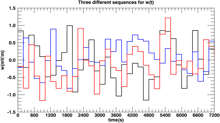
FIGURE 1. Three different sequences of randomly generated outcomes for the white noise signal, w (t), are represented in black, blue and red over a 2-h time interval. The signal is updated every T = 200 s. The expected (i.e., average) value is 0 mV/m, and the standard deviation is set to 0.5 mV/m.

Initial condition: To solve numerically Eq. 28, we consider a simple initial condition, assuming that:

- Particles are present homogeneously at all MLTs at 3.8RE and above (up to 7 RE).

- Particles are also present homogeneously in an area mimicking a localized injection, extending from r=2.5RE to r=3.8RE, and initially centered around 00:00 MLT (from 22:15 to 01:45).

The distribution function, F, is chosen to be initially constant and normalized (= 1) at all locations where particles are present. It is set to zero otherwise.

Method for numerical simulation: To solve numerically Eq. 28, we use an operator splitting method. At each time step, we first solve the transport part of the equation, using the method of characteristics. We then use the updated function to solve the diffusive part of the equation, using an explicit scheme for the sake of simplicity. We record the value of the distribution function, F, every 5 min over a 24-h interval.

4.2 Results

4.2.1 Comparison between the results of the test particle experiments and the solution of the drift-diffusion equation

We compare: a) the outputs of the particle tracking experiment with b) the solution of Eq. 28. First, we focus on one location (L = 3.5 ± 0.05 and 22:00 MLT ± 00:15): We record the time evolution of the distribution functions derived from the drift-diffusion equation and from the particle tracking experiment. The results, presented in Figure 2, highlight the consistency of the two approaches. The location is initially out of the artificial injection region thus Ft=0=0. As the particles drift eastwards starting from the midnight region, no particles are visible for a moment. Then, they briefly drift through the location, creating a transient peak in the distribution function, and so on. Figure 2 shows how the distribution function oscillates at the trapped particles’ unperturbed drift frequency. With time, the magnitude of the peak decreases, and the width of the peak increases: This is due to the combined effects of radial and azimuthal diffusions. In parallel, new particles transported radially from L ≥ 3.8 fill the region: The drift-averaged minimum of the distribution function increases with time. After some time, the drift-periodic signature disappears and the regime is purely diffusive. In other words: In this numerical experiment, the radial diffusion equation represents a valid description of the system after ∼15 h at L = 3.5 (or about 9 drift periods for the population considered). For shorter times, it is necessary to use the drift-diffusion equation to represent the time evolution of drift echoes. In general, we expect the magnitude of the typical phase-mixing time scale to be a function of: (a) the initial condition for the distribution function (the more MLT-localized the inhomogeneity, the longer it will take to cover all MLT sectors), (b) the magnitude of the diffusion coefficients (the higher the coefficient, the most efficient at smoothing MLT-dependent fluctuations, thus the shorter the characteristic time for phase mixing) and (c) the drift frequency (the higher the drift frequency, the shorter the characteristic time for phase mixing).

FIGURE 2
www.frontiersin.org

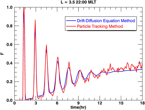
FIGURE 2. Time evolution of the distribution function centered at L = 3.5 and 22:00 MLT. The magnitude of the flux oscillation characteristic of trapped particle injections decreases with time until it vanishes after a time characteristic of phase mixing. This figure compares numerical results from (in red) a test particle simulation and (in blue) the solution of the drift-diffusion equation. It illustrates the transition from a drift-dominated regime (with the presence of drift periodic oscillations in the distribution function) to a diffusion-dominated regime (characterized by a slow and steady variation of the distribution function).

4.2.2 Visualization of the solution of the drift-diffusion equation

A 2D video of the simulation run for the solution of the drift-diffusion equation over a 24 h interval is provided in Supplementary Material. Two screenshots (at t = 3:00 h and t = 10:00 h) are provided in Figure 3.

FIGURE 3
www.frontiersin.org

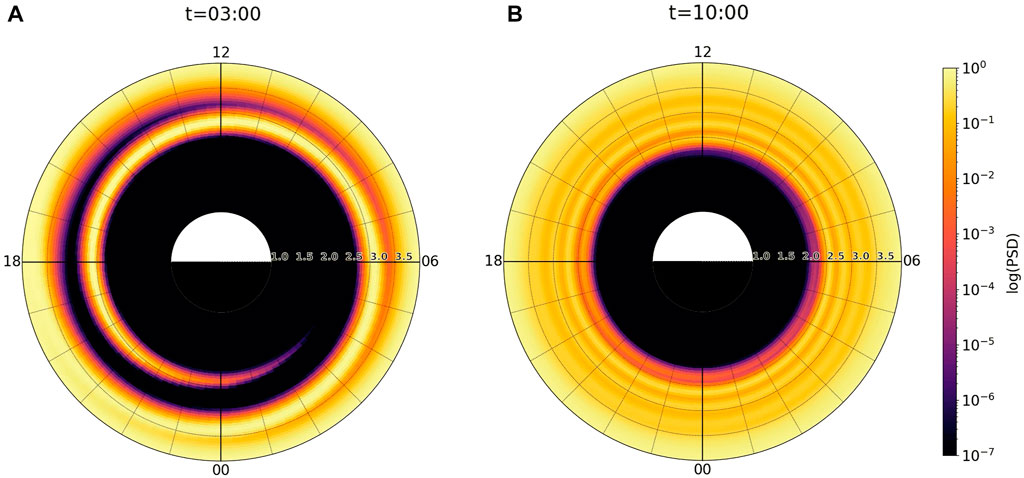
FIGURE 3. Time evolution of a distribution function (initially centered around 00:00 MLT for 2.5RE<r < 3.8RE, and constant at all MLTs for r3.8RE) (A) At t = 3:00 h, the MLT-dependent structure is visible. It creates a spiral around the Earth due to the L-dependence of the drift frequency. As a result, the distribution function is strongly dependent on MLT for r between ∼ 2.5RE and 3.8RE (B) At t = 10:00 h, the MLT-dependent structure has disappeared: The distribution function is barely dependent on MLT. The effect of transport on radiation belt intensity is now more consistent with the radial diffusion paradigm.

From the video, it is clear that the effect of the azimuthal drift on radiation belt intensity is at first more striking than the effects of radial and azimuthal diffusion. That said, drift alone would only lead to trajectories wrapping around, meaning that the distribution function would only become more structured. Radial and azimuthal diffusions act to smooth out the MLT-dependent structure, dampening it until it disappears and the distribution becomes independent of MLT. This phase-mixing process is consistent with observations. It allows for the transition from a drift-dominated regime to a diffusion-dominated regime.

5 Conclusion

We have shown how the drift-diffusion equation is capable of modeling phase mixing, allowing for a transition from drift-resolved structures (e.g., drift-periodic fluctuations associated with MLT-localized sources or losses) to the standard radial diffusion framework. We illustrated our case using simple assumptions, focusing on the magnetic equator of a dipole field and modeling electric potential fluctuations by a white noise. A next step of physical importance is to model the effect of the thermospheric wind driven electric field fluctuations on radiation belt dynamics. Indeed, electric potential fluctuations are present in the inner belt. They are viewed as the primary driver of radial diffusion in this region (e.g., O’Brien et al., 2016). In particular, electric fluctuations associated with quiet time wind dynamo have significant day-to-day variability, even during geomagnetically quiet periods (e.g., Fejer, 1993). Thermospheric wind driven electric fields are also known to shape the inner belt drift shells (Lejosne et al., 2021). Future work should consist of determining a more realistic form for the electric perturbation using information on thermospheric wind driven electric field fluctuations. Going back to the general expression of the drift-diffusion equation, future work should also consist of determining the various transport and diffusion coefficients in the presence of a time varying magnetic field. Once realistic inputs, including localized transport and diffusion coefficients, are determined, the drift-diffusion equation will enable operational radiation belt modeling with a better spatiotemporal resolution than current radial diffusion models.

Data availability statement

The raw data supporting the conclusion of this article will be made available by the authors, without undue reservation.

Author contributions

We describe contributions to the paper using the CRediT (Contributor Roles Taxonomy) categories (Brand et al., 2015). Conceptualization, Writing—Original Draft: SL and JA Writing—Review and Editing: All authors. Visualization: SL and SW. All authors contributed to the article and approved the submitted version.

Funding

SL work was performed under NASA Grant Awards 80NSSC18K1223 and 80NSSC20K1351. SW work was performed under NASA Grant Award 80NSSC20K1351. JA was supported by NASA grant 80NSSC20K1270, AFOSR grant 22RVCOR002, and the Space Vehicles Directorate of the Air Force Research Laboratory.

Conflict of interest

The authors declare that the research was conducted in the absence of any commercial or financial relationships that could be construed as a potential conflict of interest.

Publisher’s note

All claims expressed in this article are solely those of the authors and do not necessarily represent those of their affiliated organizations, or those of the publisher, the editors and the reviewers. Any product that may be evaluated in this article, or claim that may be made by its manufacturer, is not guaranteed or endorsed by the publisher.

Author disclaimer

The views expressed are those of the authors and do not reflect the official guidance or position of the United States Government, the Department of Defense or of the United States Air Force. The appearance of external hyperlinks does not constitute endorsement by the United States Department of Defense (DoD) of the linked websites, or the information, products, or services contained therein. The DoD does not exercise any editorial, security, or other control over the information you may find at these locations.

Supplementary material

The Supplementary Material for this article can be found online at: https://www.frontiersin.org/articles/10.3389/fspas.2023.1232512/abstract#supplementary-material

References

Albert, J. M. (2018). Diagonalization of diffusion equations in two and three dimensions. J. Atmos. Solar-Terrestrial Phys. 177, 202–207. doi:10.1016/j.jastp.2017.08.008

CrossRef Full Text | Google Scholar

Albert, J. M., and Young, S. L. (2005). Multidimensional quasi-linear diffusion of radiation belt electrons. Geophys. Res. Lett. 32, L14110. doi:10.1029/2005GL023191

CrossRef Full Text | Google Scholar

Birmingham, T. J., Northrop, T. G., and Fälthammar, (1967). Charged particle diffusion by violation of the third adiabatic invariant. Phys. Fluids 10, 2389. Number 11. doi:10.1063/1.1762048

CrossRef Full Text | Google Scholar

Brand, A., Allen, L., Altman, M., Hlava, M., and Scott, J. (2015). Beyond authorship: Attribution, contribution, collaboration, and credit. Learn. Pub. 28, 151–155. doi:10.1087/20150211

CrossRef Full Text | Google Scholar

Fälthammar, C.-G. (1968), Radial diffusion by violation of the third adiabatic invariant, in Earth’s particles and fields. B. M. McCormac (New York: Reinhold), 157

Google Scholar

Fejer, B. G. (1993). F region plasma drifts over Arecibo: Solar cycle, seasonal, and magnetic activity effects. J. Geophys. Res. 98 (8), 13645–13652. doi:10.1029/93JA-00953

CrossRef Full Text | Google Scholar

Lejosne, S., Fedrizzi, M., Maruyama, N., and Selesnick, R. S. (2021). Thermospheric neutral winds as the cause of drift shell distortion in Earth’s inner radiation belt. Front. Astron. Space Sci. 8, 725800. doi:10.3389/fspas.2021.725800

CrossRef Full Text | Google Scholar

Lejosne, S., and Albert, J. M. (2023). Drift phase resolved diffusive radiation belt model: 1. Theoretical framework. Front. Astron. Space Sci. 10, 1200485. doi:10.3389/fspas.2023.1200485

CrossRef Full Text | Google Scholar

Lejosne, S., and Kollmann, P. (2020). Radiation belt radial diffusion at Earth and beyond. Space Sci. Rev. 216, 19. doi:10.1007/s11214-020-0642-6

CrossRef Full Text | Google Scholar

O'Brien, T. P., Claudepierre, S. G., Guild, T. B., Fennell, J. F., Turner, D. L., Blake, J. B., et al. (2016). Inner zone and slot electron radial diffusion revisited. Geophys. Res. Lett. 43, 7301–7310. doi:10.1002/2016GL069749

CrossRef Full Text | Google Scholar

Roederer, J. G. (1970). Dynamics of geomagnetically trapped radiation. Heidelberg: Springer Berlin. doi:10.1007/978-3-642-49300-3

CrossRef Full Text | Google Scholar

Schulz, M., and Lanzerotti, L. J. (1974). Particle diffusion in the radiation belts. Berlin: Springer. doi:10.1007/978-3-642-65675-0

CrossRef Full Text | Google Scholar

Selesnick, R. S. (2012). Atmospheric scattering and decay of inner radiation belt electrons. J. Geophys. Res. 117, A08218. doi:10.1029/2012JA017793

CrossRef Full Text | Google Scholar

Tao, X., Albert, J. M., and Chan, A. A. (2009). Numerical modeling of multidimensional diffusion in the radiation belts using layer methods. J. Geophys. Res. 114, A02215. doi:10.1029/2008JA013826

CrossRef Full Text | Google Scholar

Tao, X., Chan, A. A., Albert, J. M., and Miller, J. A. (2008). Stochastic modeling of multidimensional diffusion in the radiation belts. J. Geophys. Res. 113, A07212. doi:10.1029/2007JA012985

CrossRef Full Text | Google Scholar

Tao, X., Zhang, L., Wang, C., Li, X., Albert, J. M., and Chan, A. A. (2016). An efficient and positivity-preserving layer method for modeling radiation belt diffusion processes. J. Geophys. Res. Space Phys. 121, 305–320. doi:10.1002/2015JA022064

CrossRef Full Text | Google Scholar

Ukhorskiy, A., Sitnov, M., Mitchell, D., Takahashi, K., Lanzerotti, L. J., and Mauk, B. H. (2014). Rotationally driven ‘zebra stripes’ in Earth’s inner radiation belt. Nature 507, 338–340. doi:10.1038/nature13046

PubMed Abstract | CrossRef Full Text | Google Scholar

Whipple, E. C. (1978). U, B, K) coordinates: A natural system for studying magnetospheric convection. J. Geophys. Res. 83 (A9), 4318–4326. doi:10.1029/JA083iA09p04318

CrossRef Full Text | Google Scholar

Appendix

We explain how we derived the expressions for r2, φ2, and rφ (Eq. 11), in order to obtain the diffusion coefficients required to solve the drift-diffusion equation.

A first-order Taylor expansion for the expressions of the total variations in radial and azimuthal locations (Eq. 10) yields:

r=ro3BERE3tt+twusinφo+Ωuduφ=Ωt+3MγoqBERE323MBERE3γo2Eoro3tt+ttuwxsinφo+Ωxdxdu+ro2BERE3tt+twucosφo+Ωudu(A1)

where ro,φo,γo are the values for the radial and azimuthal locations, and Lorentz factor, at time, t, respectively.

The expression for the ensemble average of the square of the total variation of the radial displacement is:

r2=ro6BE2RE6tt+ttt+twuwvsinφo+Ωusinφo+Ωvdudv(A2)

Since ΩΔt1, the variation in phase is not significant, and Eq. A2 becomes

r2=ro6sin2φoBE2RE6tt+ttt+twuwvdudv(A3)

Since the signal w is a piecewise constant function, we have that:

wu=wiforiTu<i+1T(A4)

And by definition of the white noise sequence, wiwj=W2δij, where δij is the Kronecker delta. As a result, expressing the time interval, t, as t=NT+k, where N is an integer, and 0<k<T:

r2=ro6W2sin2φoBE2RE6NT2+k2ro6W2Tsin2φoBE2RE6t(A5)

As a result:

r2=r2t=ro6W2TBE2RE6sin2φo(A6)

A similar approach allows for a computation of φ2, and rφ2 as first order functions of t, yielding analytical expressions for φ2, and rφ. Alternatively, the total variation in phase, φ, can also be related the total variation in radial displacement, r, and the time variation, t, by considering a multivariate Taylor expansion for the expression of total energy conservation (e.g., Whipple, 1978):

Ekro+r,φo+φ,t+t+qVro+r,φo+φ,t+t=Ekro,φo,t+qVro,φo,t(A7)

where Ek=Eo1+2MB/Eo1 is the kinetic energy, with Eo the rest mass energy.

The formula provided Eq. A6 is not dependent on the energy of the particles considered, provided that the drift period is very long in comparison with the updating time,
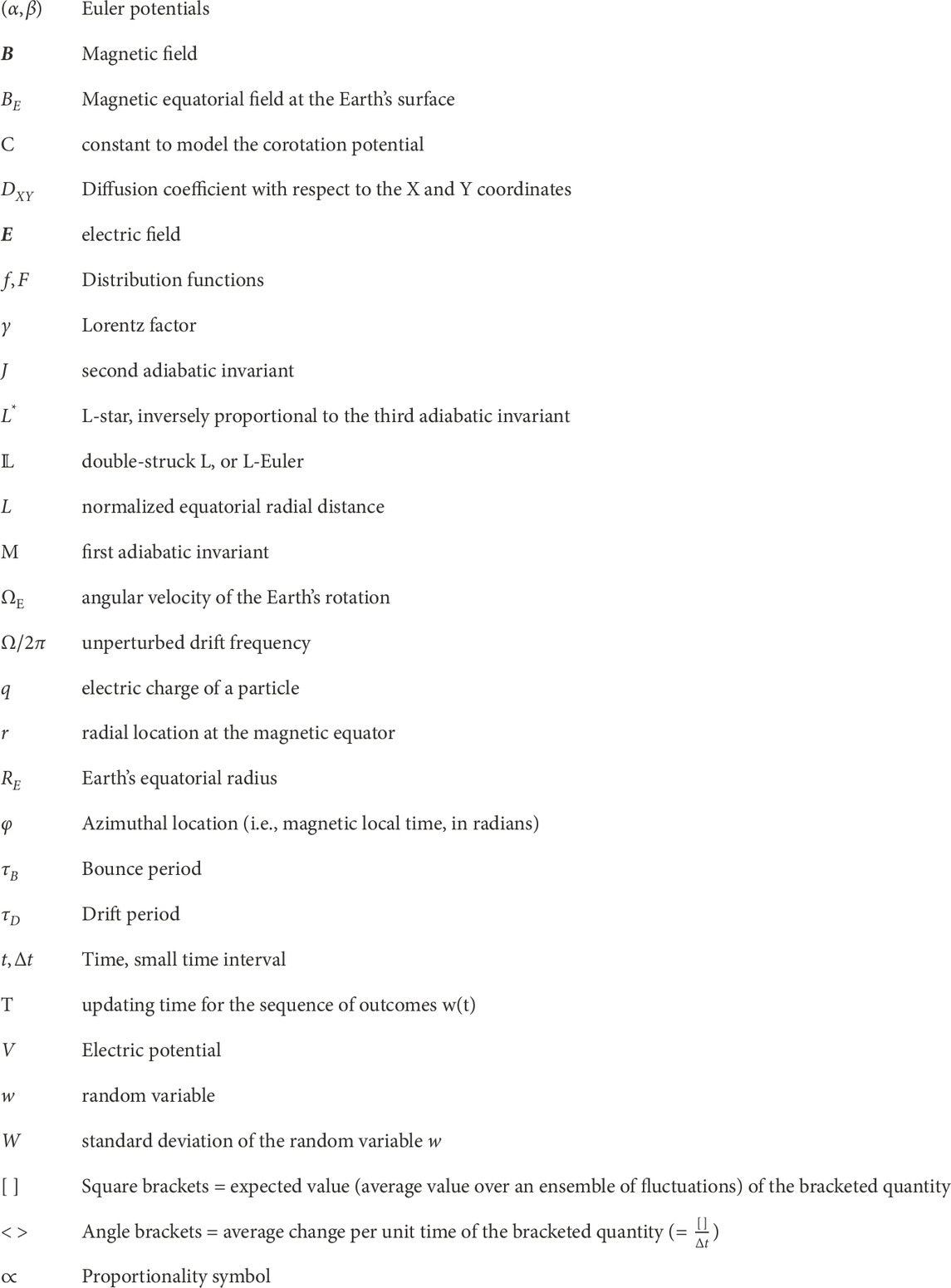
 T. If we were to consider particles of higher energies, with a drift period smaller than the updating time, T, the magnitude of the radial diffusion coefficient would drop, in accordance with theoretical expectations. Indeed, with t=k<T, N=0, and r2 Eq. (A5) would become proportional to W2t2<W2Tt. In parallel, the ensemble average of the signal, w, would not be 0 anymore during t: this means that the effects of field fluctuations would be accounted for through the transport coefficients, L˙ and φ˙ (Eq. 9).

Glossary

Keywords: radiation belts, fokker-planck equation, adiabatic invariants, radial transport, radial diffusion, azimuthal diffusion, cross-terms, electric fields

Citation: Lejosne S, Albert JM and Walton SD (2023) Drift phase resolved diffusive radiation belt model: 2. implementation in a case of random electric potential fluctuations. Front. Astron. Space Sci. 10:1232512. doi: 10.3389/fspas.2023.1232512

Received: 31 May 2023; Accepted: 13 July 2023;
Published: 08 August 2023.

Edited by:

Qianli Ma, Boston University, United States

Reviewed by:

Greg Cunningham, Los Alamos National Laboratory (DOE), United States
Xin Tao, University of Science and Technology of China, China

Copyright © 2023 Lejosne, Albert and Walton. This is an open-access article distributed under the terms of the Creative Commons Attribution License (CC BY). The use, distribution or reproduction in other forums is permitted, provided the original author(s) and the copyright owner(s) are credited and that the original publication in this journal is cited, in accordance with accepted academic practice. No use, distribution or reproduction is permitted which does not comply with these terms.

*Correspondence: Solène Lejosne, solene@berkeley.edu

Disclaimer: All claims expressed in this article are solely those of the authors and do not necessarily represent those of their affiliated organizations, or those of the publisher, the editors and the reviewers. Any product that may be evaluated in this article or claim that may be made by its manufacturer is not guaranteed or endorsed by the publisher.