Dispersive propagation of nuclear electromagnetic pulse in the ionosphere

Introduction: On the propagation path to the satellite, the ionosphere will distort the nuclear electromagnetic pulse (NEMP) and change its physical properties.

Methods: This paper proposes a method for calculating the propagation of NEMP to the satellite. The method decomposes NEMP into the superposition of simple harmonic waves, and each simple harmonic wave is calculated separately in the ionosphere. With the consideration of different time of arrival and critical frequency of the ionosphere, the NEMP after propagating in the ionosphere is obtained by superposition of simple harmonic waves in time domain rather than the inverse Fourier transform which will erase the time domain information.

Results: The results show that NEMP is dispersive in ionosphere with the pulse broadened, the speeds changed and the bandwidth narrowed. The time-frequency spectrum can provide the frequency band where the signal energy is located.

Discussion: Our proposed method provides a simple and effective way to calculate the NEMP propagation in the ionosphere, which should afford help to the design of NEMP receivers and the selection of satellite orbit altitude.

1 Introduction

Nuclear electromagnetic pulse (NEMP) is one of the important effects of nuclear explosions, with fast propagation speed, high peak value, wide frequency band, wide coverage and other characteristics. NEMP is appropriate for use as a detection target for space-based nuclear explosion monitoring systems. As a consequence of the Comprehensive Nuclear Test Ban Treaty, non-nuclear experimental and theoretical efforts are expanded to study and observe the NEMP phenomenology and to develop appropriate descriptive models. For the non-nuclear experimental efforts, especially in space-based NEMP explosion monitoring, in 1997, the United States launched a near Earth satellite, FORTE (Fast On orbit Recording of Transient Events), with an optical and radio frequency detection system. The satellite is equipped with a 90 MHz receiver and a pair of 20 MHz receivers, both of which can be tuned in the range of 30–300 MHz. The FORTE received the pulse signal sent by the ground electromagnetic pulse generator (Massey et al., 1998). After band-pass filtering and converting it into a digital signal, it was transmitted back to the ground for analysis, so as to obtain the ionospheric information of the propagation path (Roussel-Dupre et al., 2001; Huang and Roussel-Dupre, 2005; Minter et al., 2007) and carry out the ground signal source positioning algorithm (Jacobson and Shao, 2001). With the above mentioned techniques, FORTE has the ability to detected the NEMP signal.

Theoretical methods for studying NEMP propagation can be classified into two categories: time-domain methods and frequency-domain methods. For the time-domain methods, the Maxwell equations are the most essential parts. The electric field components and magnetic field components are calculated with appropriate current sources, medium parameters and boundary conditions. The widely used numerical calculation method is Finite Difference Time Domain (FDTD) method. With this method, the physical process of electromagnetic pulse excited by Compton electron currents is simulated (Meng et al., 2003; Meng, 2013). The discrete iterative equations for the electromagnetic field components are presented in the CPML (Convolutional Perfect Matched Layer) media under the two-dimension and three-dimension prolate-spheroidal coordinate system (Gao et al., 2005a; Gao et al., 2005b). Chen et al. derived the time-domain difference equations for the interaction between ionosphere and electromagnetic pulse (Chen et al., 2011). Those results show that the combination of ionospheric time-domain calculation method and NEMP calculation method is reasonable and effective. However, FDTD method is suitable for the electromagnetic field calculation of subtle structures, and it takes a very long time for the calculation of long distance electromagnetic pulse propagation.

In frequency domain methods, the ionosphere is considered as the transfer function, and the Fourier transform is used to obtain the spectrum of NEMP signal. The amplitude and phase of each frequency component after propagation in the ionosphere are calculated respectively. Then, the inverse Fourier transform is used to obtain the NEMP signal received at the satellite orbit (Meng et al., 2004; Yao et al., 2019). Nevertheless, the Fourier transform will erase the time domain information of NEMP signal, and the inverse Fourier transform ignores that the different frequency components have different speeds in dispersive material.

This paper proposes a method for NEMP propagation in the ionosphere. The method decomposes the NEMP signal into the superposition of simple harmonic waves. The propagation of each simple harmonic wave in the ionosphere is calculated separately. With the consideration of the time differences among the simple harmonic waves, the NEMP signal is obtained by superposition of simple harmonic waves after propagation in the ionosphere. This paper is organized as follows: In Section 2, the model of ionosphere, decomposition of NEMP and superposition of simple harmonic waves are presented. In Section 3, the waveforms chosen for simulation are introduced and the results and discussion are presented. In the last section, we conclude this paper and present the applications.

2 Methods

2.1 Model of ionosphere

2.1.1 Multilayer model

The multilayer model is used for calculation, as a result of the non-uniform distribution of the plasma density in the ionosphere. Each layer is considered to be uniform and has a thickness of $\Delta h$, as is shown in Figure 1. It is assumed that the $p_0$ layer is vacuum due to the negligible plasma density.

FIGURE 1

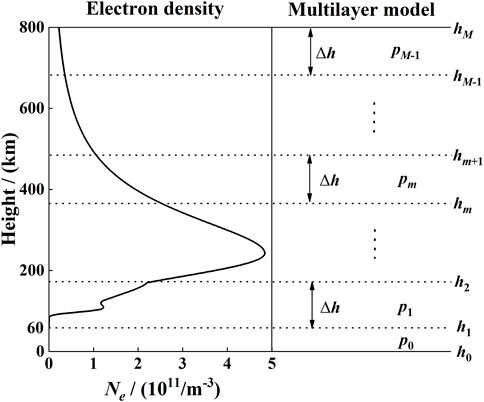
FIGURE 1. Ionospheric electron density profile and multilayer model.

The plasma frequency of the ionosphere is $f_p=\sqrt{N_e{e}^2/4{\pi }^2{m}_e{\epsilon }_0}$, where $e=1.602176634\times {10}^{-19}\mathrm{C}$ is the charge of electron, $m_e=9.10956\times {10}^{-31}\text{kg}$ is the mass of electron, ${\epsilon }_0=8.854187817\times {10}^{-12}\mathrm{F}/\mathrm{m}$ is the vacuum permittivity, and $N_e$ is the electron density.

2.1.2 Critical frequency

$N_e$ increases with the increase of altitude, and after reaching the peak $N_{em}$, $N_e$ starts to decrease. The plasma frequency corresponding to $N_{em}$ is the critical frequency, namely, $f_c=\sqrt{N_{em}{e}^2/4{\pi }^2{m}_e{\epsilon }_0}$. The frequency components below the critical frequency cannot continue to propagate upward.

2.1.3 Collision frequency

Particles in the ionosphere are in thermal motion and inevitably collide. Frequencies of electron-neutral and electron-ion collisions affect the ionosphere propagation of the signals (He and Zhao, 2009).

The collision frequencies of electron-neutral particle include.

(1) Collision frequency of electrons with Nitrogen molecules $\left({\mathrm{N}}_2\right)$

${\nu }_{e,{\mathrm{N}}_2}=2.33\times {10}^{-17}n\left({\mathrm{N}}_2\right)\left[1-1.21\times {10}^{-4}{T}_e\right]T_e(1)$

(2) Collision frequency of electrons with Oxygen molecules $\left({\mathrm{O}}_2\right)$

${\nu }_{e,{\mathrm{O}}_2}=1.82\times {10}^{-16}n\left({\mathrm{O}}_2\right)\left[1+0.036T_e^{1/2}\right]T_e^{1/2}(2)$

(3) Collision frequency of electrons with Oxygen atoms $\left(\mathrm{O}\right)$

${\nu }_{e,\mathrm{O}}=2.65\times {10}^{-16}n\left(\mathrm{O}\right)T_e^{1/2}(3)$

(4) Collision frequency of electrons with Helium atoms $\left(\text{He}\right)$

${\nu }_{e,\text{He}}=4.6\times {10}^{-16}n\left(\text{He}\right)T_e^{1/2}(4)$

From Eqs 1–4, $T_e$ is the electron temperature (in eV, 1 eV = 11,600 K), $n\left({\mathrm{N}}_2\right)$, $n\left({\mathrm{O}}_2\right)$, $n\left(\mathrm{O}\right)$, $n\left(\text{He}\right)$ are the density of neutral particles ${\mathrm{N}}_2$, ${\mathrm{O}}_2$, $\mathrm{O}$, $\text{He}$, respectively.

The collision frequency of electron-ion is

${\nu }_{e,i}=5.45\times {10}^{-5}n\left(i\right)T_e^{-3/2}(5)$

where ${\nu }_{e,i}$ is the collision frequency of electrons with the ion i, which represents $\mathrm{N}{\mathrm{O}}^{+}$, ${\mathrm{O}}_2^{+}$, ${\mathrm{O}}^{+}$ in this paper. $n\left(i\right)$ represents the density of the ion i.

The total electron collision frequency ${\nu }_e$ can be expressed as

${\nu }_e={\nu }_{e,{\mathrm{N}}_2}+{\nu }_{e,{\mathrm{O}}_2}+{\nu }_{e,\mathrm{O}}+{\nu }_{e,\text{He}}+{\nu }_{e,\mathrm{N}{\mathrm{O}}^{+}}+{\nu }_{e,{\mathrm{O}}_2^{+}}+{\nu }_{e,{\mathrm{O}}^{+}}(6)$

2.1.4 Refraction index

The propagation of electromagnetic waves in the ionosphere follows the Appleton-Lassen equation. In the absence of geomagnetic field (Huang, 2000), the refraction index can be expressed by

$n=\mu -\mathrm{i}\eta =\sqrt{1-\left(X/\left(1-\mathrm{i}Z\right)\right)}(7)$

where $\mu$ and $\eta$ are real and imaginary parts, respectively; $X=f_p^2/f^2$; $Z={\nu }_e/2\pi f$; $f$ is the frequency of the simple harmonic wave.

In vacuum, the speed of a simple harmonic wave $v$ is equal to the speed of light $c$, namely, $v=c\approx 3\times {10}^8\mathrm{m}/\mathrm{s}$. In the ionosphere considering collisions, the phase speed $v_p$ can be expressed by (Liu et al., 2010)

$v_p=\frac{1}{{{\mu }_0\epsilon }_{real}}\sqrt{2/\left(\sqrt{1+{\left(\mathrm{\sigma }/2\pi f{\epsilon }_{real}\right)}^2}+1\right)}(8)$

where, $\mathrm{\sigma }=N_e{e}^2/m_e{\nu }_e$ is the conductivity. ${\epsilon }_{real}$ is the real part of $\epsilon ,$ where $\epsilon ={\epsilon }_0\left[1+{\left(2\pi f_p\right)}^2/2\pi f\left(i{v}_e-2\pi f\right)\right].$ The item $\sqrt{2/\left(\sqrt{1+{\left(\mathrm{\sigma }/2\pi f{\epsilon }_{real}\right)}^2}+1\right)}$ is always great than 1, resulting in $v_p<c$. According to Eq. 8, as the frequency $f$ increases, $v_p$ also increases, shown in Figure 2.

FIGURE 2

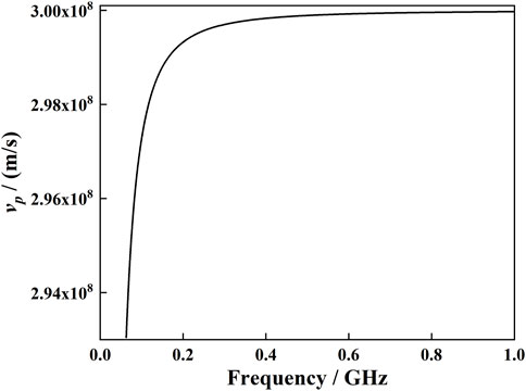
FIGURE 2. Speed of different frequencies of simple harmonic waves.

The propagation time in each layer of ionosphere is given by

$t=\Delta h/v_p(9)$

In vacuum, the amplitude is a function of distance from the source point

$E_1=E_0/r(10)$

where $E_0$ is the initial amplitude, $E_1$ is the amplitude at $r$ distance from the source point.

In the ionosphere, the attenuation of amplitude with distance $r$ can be expressed as

$E_2=E_0{\mathrm{e}}^{-\beta r}(11)$

where $E_2$ is the amplitude at $r$ distance from the source point; $\beta =2\pi f\eta /c$ is the attenuation coefficient with frequency $f$.

2.2 Dispersive propagation in the ionosphere

2.2.1 Decomposition of NEMP

In the light of Eqs 7–11, the influence of the ionosphere differ with the frequency $f$. Therefore, we decompose NEMP into $K$ simple harmonic waves, and study the propagation of each simple harmonic wave in the ionosphere.

The Fourier transform is applied to $E\left(t\right)$ and the signal is converted from the time domain $E\left(t\right)$ to the frequency domain $E\left(f\right)$. The complex value corresponding to frequency $f_k$ is $E\left(f_k\right)=a_k+\mathrm{i}{b}_k$. The simple harmonic wave decomposed from $E\left(t\right)$ can be described as

$e_k\left(t\right)=E_k\cos \left(2\pi f_{k}t+{\phi }_k\right)(12)$

where $f_k$ is the frequency, $E_k=\sqrt{a_k^2+b_k^2}$ and ${\phi }_k=\arctan$ ($b_k/a_k$) are the initial amplitude and phase, respectively. The superposition of all simple harmonics can be expressed as

$E^{\prime }\left(t\right)=e_1\left(t\right)+e_2\left(t\right)+\dots +e_K\left(t\right)={\displaystyle {\sum }_{k=1}^K}{e}_k\left(t\right)={\displaystyle {\sum }_{k=1}^K}{E}_k\cos \left(2\pi f_{k}t+{\phi }_k\right)(13)$

where $e_1\left(t\right)$ is the simple harmonic wave with highest frequency $f_1$, and $e_K\left(t\right)$ is the simple harmonic wave with the lowest frequency $f_K$.

2.2.2 A simple harmonic wave propagation in the ionosphere

2.2.2.1 Propagation from ${\mathit{h}}_{\mathbf{0}}$ to ${\mathit{h}}_{\mathbf{1}}$

For a simple harmonic wave with frequency $f_k$, when propagating vertically upward from $h_0$ to the bottom layer $h_1$ of the ionosphere, where there is no plasma, the propagation time is calculated by

$t_{k0}=h_1/c(14)$

and the amplitude is calculated by

$E_k^{\prime }=E_k/h_1(15)$

The expression is derived from Eq. 12 as

$e_k\left(t\right)=\frac{E_k}{h_1}\cos \left[2\pi f_k\left(t+t_{k0}\right)+{\phi }_k\right](16)$

2.2.2.2 Propagation from ${\mathit{h}}_{\mathbf{0}}$ to ${\mathit{h}}_{\mathbf{2}}$

When propagating from $h_1$ to $h_2$, i.e., in $p_1$ layer, the refraction index of $p_1$ layer is expressed by

$n_{k1}={\mu }_{k1}-\mathrm{i}{\eta }_{k1}(17)$

The propagation time is calculated by

$t_{k1}=\Delta h/v_{k1}(18)$

The absorption loss can be derived from Eqs 10, 11

$E_k^{\prime }=\frac{E_k}{h_2}{\mathrm{e}}^{-{\beta }_{k1}\Delta h}(19)$

where ${\beta }_{k1}=2\pi f_k{\eta }_{k1}/c$ is the attenuation coefficient in $p_1$ layer, Eq. 16 is then expressed as

$e_k\left(t\right)=\frac{E_k}{h_2}{\mathrm{e}}^{-{\beta }_{k1}\Delta h}\cos \left[2\pi f_k\left(t+t_{k0}+t_{k1}\right)+{\phi }_k\right](20)$

2.2.2.3 Propagation from ${\mathit{h}}_{\mathbf{0}}$ to ${\mathit{h}}_{\mathit{M}}$

By analogy, when the simple harmonic wave $e_k\left(t\right)$ propagates to the height $h_M$, the expression is

$e_k\left(t\right)=\frac{E_k}{h_M}{\mathrm{e}}^{-{\displaystyle {\sum }_{m=1}^{M-1}}\left({\beta }_{km}\Delta h\right)}\cos \left[2\pi f_k\left(t+{\displaystyle {\sum }_{m=0}^{M-1}}{t}_{km}\right)+{\phi }_k\right](21)$

where ${\beta }_{km}=2\pi f_k{\eta }_{km}/c$ is the attenuation coefficient in $p_m$ layer, $t_{km}=\Delta h/v_{km}$ is the propagation time in $p_m$ layer, and ${\displaystyle {\sum }_{m=0}^{M-1}}{t}_{km}$ is the propagation time from $h_0$ to $h_M$.

2.2.2.4 Definition domain

Each simple harmonic wave has the same duration $T$. The time difference $\Delta t_k$ between $e_1\left(t\right)$ and $e_k\left(t\right)$, propagating from $h_0$ to $h_M$, is given by

$\Delta t_k={\displaystyle {\sum }_{m=0}^{M-1}}{t}_{km}-{\displaystyle {\sum }_{m=0}^{M-1}}{t}_{1m}={\displaystyle {\sum }_{m=0}^{M-1}}\left(t_{km}-t_{1m}\right)(22)$

Equation 22 represents that when $e_1\left(t\right)$ reaches $h_M$, $e_k\left(t\right)$ needs $\Delta t_k$ to reach it. Simple harmonic waves of different frequencies propagation in the ionosphere are shown in Figure 3.

FIGURE 3

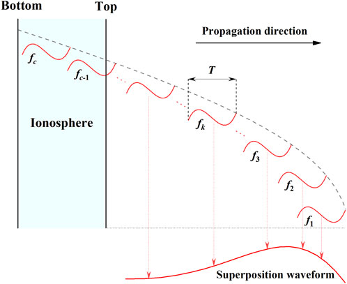
FIGURE 3. Simple harmonic waves of different frequencies propagation in the ionosphere.

Taking the moment when $e_1\left(t\right)$ reaches $h_M$ as the zero moment, then the time domain of $e_k\left(t\right)$ is defined as

$\Delta t_k\le t_k\le T+\Delta t_k(23)$

In particular, the time domain of $e_1\left(t\right)$ is defined as

$0\le t_1\le T(24)$

2.2.3 Superposition of simple harmonic waves

The ionosphere will reflect the simple harmonic waves with frequencies below the critical frequency $f_c$. The simple harmonic waves that can penetrate the ionosphere are $e_1\left(t\right)$, $e_2\left(t\right)$, …, $e_k\left(t\right)$, …, $e_c\left(t\right)$. $e_c\left(t\right)$ is the last simple harmonic wave that can penetrate the ionosphere. $e_{c+1}\left(t\right)$, …, $e_K\left(t\right)$ will be reflected by the ionospheric electron frequency peak (foF2).

With the consideration of the critical frequency and the different definition domain, the simple harmonic waves $e_1\left(t\right)$, $e_2\left(t\right)$, …, $e_c\left(t\right)$ are superimposed, so NEMP signal $E\left(t\right)$ that propagates from $h_0$ vertically upward to $h_M$ is finally described as

$E^{″}\left(t\right)={\displaystyle {\sum }_{k=1}^c}{e}_k\left(t\right)={\displaystyle {\sum }_{k=1}^c}\left\{\frac{E_k}{h_M}{\mathrm{e}}^{-{\displaystyle {\sum }_{m=1}^{M-1}}\left({\beta }_{km}\Delta h\right)}\cos \left[2\pi f_k\left(t+{\displaystyle {\sum }_{m=0}^{M-1}}{t}_{km}\right)+{\phi }_k\right]\right\}(25)$

3 Simulation

The NEMP is emitted at the ground and is received at an altitude of 800 km and let $\Delta h=1$ km. The data of electron density and ions density are downloaded from the International Reference Ionosphere (International Reference Ionosphere - IRI (2016) | CCMC (nasa.gov)). The data of neutral particle density are downloaded from the NRLMSISE-00 Atm Model (NRLMSISE-00 Atm Model | CCMC (nasa.gov)). The electron density of the ionosphere as a function of altitude is plotted in Figure 1. The parameters of ionosphere are shown in Table 1.

TABLE 1

TABLE 1. Parameters of ionosphere.

3.1 Simulation waveform

We choose Bell Laboratory pulse as the simulation waveform. The first reason is that the method proposed in this paper is to study the dispersion of NEMP in the ionosphere, rather than the generation of NEMP. Therefore, the simulation waveform can be adjusted and replaced to meet the needs of the simulation. The second reason is that it is easier to be simulated, which facilitates post-calculation analysis.

Bell Laboratory pulse is represented by the double exponential function

$E\left(t\right)=k{E}_0\left({\mathrm{e}}^{-\alpha t}-{\mathrm{e}}^{-\beta t}\right)(26)$

where $E_0$ is the maximum amplitude, $k={\left({\mathrm{e}}^{-\alpha t_p}-{\mathrm{e}}^{-\beta t_p}\right)}^{-1}$ is the modifying factor, $\alpha$ and $\beta$ are the parameters characterizing both the rise time and fall time simultaneously, $t_p=\left(\ln \beta -\ln \mathrm{\alpha }\right)/\left(\beta -\mathrm{\alpha }\right)$ is the peak time.

Parameters of Bell Laboratory pulse are shown in Table 2. The original waveform $E\left(t\right)$ and superposition waveform $E^{\prime }\left(t\right)$ which is obtained from Eq. 13, are shown in Figure 4. The relative error is less than 1 × 10⁻¹¹%. Compared to the order of original waveform, the error is negligible.

TABLE 2

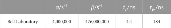
TABLE 2. Parameters of Bell Laboratory pulse.

FIGURE 4

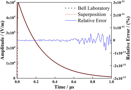
FIGURE 4. Bell Laboratory pulse, superposition waveform and the relative error.

3.2 Results and discussion

Let $E_B\left(t\right)$ represents the Bell Laboratory pulse after propagation in the ionosphere. $E_B\left(t\right)$ becomes an oscillatory waveform with a long tail after propagation in the ionosphere, and is stretched from 1 to 30 μs. The rising edge of the envelope becomes slower, and the duration of the rising edge and the falling edge are almost the same. In addition, there is a peak time delay of 10 μs for $E_B\left(t\right)$, shown in Figure 5.

FIGURE 5

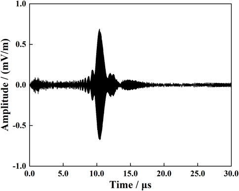
FIGURE 5. Bell Laboratory pulse after propagation in the ionosphere.

The delay can be explained with the simple harmonic waves’ arrival time differences and amplitudes, shown in Table 3. From 0 to 6 μs, the frequencies of the simple harmonic waves are all above 50 MHz, but their amplitudes are small, so the envelope of $E_B\left(t\right)$ is flat. The envelope begins to rise at 6 μs, corresponding to the arrival time of a 50 MHz harmonic wave. Simple harmonic waves with lower frequencies but larger amplitudes then arrive and superimposed one after another. The energy of the pulse accumulates and reaches the peak at 10 μs. After 10 μs, although the amplitude of the arriving simple harmonic waves is larger than those that have arrived before 10 μs, the time difference of arrival is also increasing, so that the overlap between adjacent simple harmonic waves is constantly reduced. The energy of the pulse fails to accumulate, and the envelope begins to fall.

TABLE 3

TABLE 3. Amplitudes and time differences of simple harmonic waves.

Because of the critical frequency, the simple harmonic waves below it will be reflected. The critical frequency in the ionosphere is 6.24 MHz, and there are no amplitudes below the critical frequency, which are shown in Figure 6. It should be noted that Figure 6 is the one-to-one correspondence between simple harmonic waves and their amplitudes after propagation in the ionosphere. The frequency spectrum has the same shape as the original waveform.

FIGURE 6

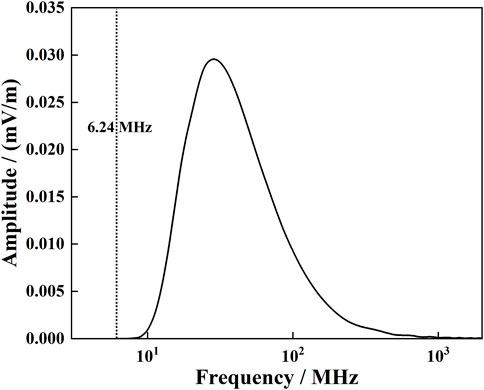
FIGURE 6. Frequency spectrum of Bell Laboratory pulse after propagation in the ionosphere.

The spectrum of the time-frequency of $E_B\left(t\right)$ shows that the simple harmonic waves with higher frequencies arrive earlier, which is consistent with the time-frequency spectrum of the signal observed by the satellite (Massey et al., 1998). The brightest area in Figure 7 represents the frequency band with the highest concentration of energy and corresponds to the peak of $E_B\left(t\right)$, too.

FIGURE 7

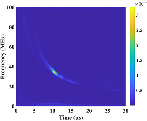
FIGURE 7. Time–frequency spectrum of Bell Laboratory pulse after propagation in the ionosphere.

Comparing the above results with other scholars’ great work (Liang and Zheng, 2009; Chen et al., 2011), our proposed method can explain the changes of waveforms after propagation in the ionosphere, such as the delay of the peak time, in light of the arrival time differences and amplitudes of simple harmonic waves. Besides, the application of inverse Fourier transform requires that the frequency components have the same wave front, in other words, the frequency components have the same propagation speed. Therefore, inverse Fourier transform is not suitable for the dispersive materials (Yao et al., 2019). Our proposed method is to superimpose the simple harmonic waves directly, which coincides with realistic physical process.

We have chosen different values of $\Delta h$ to calculate the peak value of $E_B\left(t\right)$. The results are shown in Table 4. The origin peak value of the pulse is 50,000 V/m, and peak value of the pulse after propagation in the ionosphere is in the order of mV/m. The order of amplitude of the calculation is what we care about most.

TABLE 4

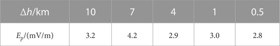
TABLE 4. Peak value and thickness of each layer.

4 Conclusion

This paper proposes a method for calculating the propagation of NEMP in the ionosphere. Our method surpasses the weakness of the inverse Fourier transform that erases the propagation time difference for different frequencies. The results show that the NEMP signal is broadened as 30 times as its original length in the ionosphere. The spectrum of NEMP signal has the shape of the original signal envelope. The obtained dispersed spectrum is consistent with the satellite observations. The method can be used for the design of the space-based NEMP detectors and satellite-ground docking experiments. The propagation model may be optimized upon receipt of downlink data from the satellite.

Data availability statement

The original contributions presented in the study are included in the article/Supplementary Material, further inquiries can be directed to the corresponding authors.

Author contributions

YLW proposed the model and the method, and wrote the paper. DHZ and ZXL ran the simulation. LHW and YW analyzed the results. TCZ and BX wrote the paper. BFC and PL did the literature review and checked the paper. All authors contributed to the article and approved the submitted version.

Funding

This paper is supported by the Strategic Priority Research Program of Chinese Academy of Sciences (Grant No. XDA17040503).

Conflict of interest

The authors declare that the research was conducted in the absence of any commercial or financial relationships that could be construed as a potential conflict of interest.

Publisher’s note

All claims expressed in this article are solely those of the authors and do not necessarily represent those of their affiliated organizations, or those of the publisher, the editors and the reviewers. Any product that may be evaluated in this article, or claim that may be made by its manufacturer, is not guaranteed or endorsed by the publisher.

References

Chen, Y., Ma, L., Zhou, H., Wu, W., Li, J., and Li, B. (2011). Calculation of high altitude nuclear electromagnetic pulse propagation in ionosphere. HIGH POWERLASER Part. BEAMS 23 (02), 441–444. doi:10.3788/hplpb20112302.0441

CrossRef Full Text | Google Scholar

Gao, C., Chen, Y., and Wang, L. (2005a). Application of CPML to two-dimension numerical simulation of nuclear electromagnetic pulse from air explosions. HIGH POWERLASER Part. BEAMS 07, 1111–1116.

Google Scholar

Gao, C., Chen, Y., and Wang, L. (2005b). The application of CPML in three-dimensional numerical simulation of low-altitude electromagnetic pulse. Chin. J. Comput. Phys. 22 (4), 292–298. doi:10.19596/j.cnki.1001-246x.2005.04.002

CrossRef Full Text | Google Scholar

He, F., and Zhao, Z. (2009). Ionospheric loss of high frequency radio wave propagated in the ionospheric regions. Chin. J. Radio Sci. 24 (04), 720–723+747.

Google Scholar

Huang, J. (2000). Correction for atmospheric refractive error of radio wave. Beijing: National Defense Industry Press.

Google Scholar

Huang, Z., and Roussel-Dupre, R. (2005). Total electron content (TEC) variability at Los Alamos, New Mexico: a comparative study: FORTE-derived TEC analysis. Radio Sci. 40 (6), RS6007. doi:10.1029/2004rs003202

CrossRef Full Text | Google Scholar

Jacobson, A. R., and Shao, X. (2001). Using geomagnetic birefringence to locate sources of impulsive, terrestrial VHF signals detected by satellites on orbit. Radio Sci. 36 (04), 671–680. doi:10.1029/2000rs002555

CrossRef Full Text | Google Scholar

Liang, R., and Zheng, Y. (2009). Calculation of nuclear electromagnetic pulse propagation into space. Nucl. Electronics& Detect. Technol. 29 (06), 1393–1396.

Google Scholar

Liu, S., Liu, S., and Hong, W. (2010). Finite difference time domain method for dispersive media. Beijing: Science Press.

Google Scholar

Massey, R. S., Knox, S. O., Franz, R. C., Holden, D. N., and Rhodes, C. T. (1998). Measurements of transionospheric radio propagation parameters using the FORTE satellite. Radio Sci. 33 (6), 1739–1753. doi:10.1029/98rs02032

CrossRef Full Text | Google Scholar

Meng, C. (2013). Numerical simulation of the HEMP environment. IEEE Trans. Electromagn. Compat. 55(3), 440–445. doi:10.1109/temc.2013.2258024

CrossRef Full Text | Google Scholar

Meng, C., Chen, Y., and Zhou, H. (2003). Effects of the HOB and the burst yield on the properties of NEMP. Chin. J. Comput. Phys. 20(2), 173–177. doi:10.19596/j.cnki.1001-246x.2003.02.016

CrossRef Full Text | Google Scholar

Meng, C., Chen, Y., Zhou, H., and Gong, J. (2004). The analysis of the propagation of transient electromagnetic pulse through ionosphere. Nucl. Electron. Detect. Technol. 24 (04), 369–372+406.

Google Scholar

Minter, C. F., Robertson, D. S., Spencer, P. S. J., Jacobson, A. R., Full-Rowell, T. J., Araujo-Pradere, E. A., et al. (2007). A comparison of Magic and FORTE ionosphere measurements. Radio Sci. 42 (3), RS3026. doi:10.1029/2006rs003460

CrossRef Full Text | Google Scholar

Roussel-Dupre, R. A., Jacobson, A. R., and Triplett, L. A. (2001). Analysis of FORTE data to extract ionospheric parameters. Radio Sci. 36 (6), 1615–1630. doi:10.1029/2000rs002587

CrossRef Full Text | Google Scholar

Yao, J., Shan, H., Cao, B., and Jiang, T. (2019), “Waveform prediction of V/UHF EMP signal propagation in the ionosphere”, in Proceedings of the 2019 IEEE Asia-Pacific Microwave Conference (APMC), Singapore, December 2019. 1062–1064.

CrossRef Full Text | Google Scholar