Analysis of the different physical mechanisms in the atypical sporadic E (Es) layer occurrence over a low latitude region in the Brazilian sector

We present a study about the atypical and spreading Sporadic E-layers (Es) observed in Digisonde data. We analyzed a set of days around space weather events from 2016 to 2018 over Cachoeira Paulista (CXP, 22.41°S, 45°W, dip ∼35°), a low-latitude Brazilian station. The inhomogeneous Es layer is associated with the auroral-type Es layer (Es_a) occurrence in this region due to the presence of South American Magnetic Anomaly (SAMA). However, we also observe that the spreading Es layers occurred days before the magnetic storms or quiet times. Also, this specific type of Es layer has some different characteristics concerning the Es_a layer. We used data from the imager, satellite, and meteor radar to understand the dynamic processes acting in this Es layer formation. Our results lead us to believe that other mechanisms affect the Es layer development. We show evidence that the instabilities added to the wind shear mechanism can cause the atypical Es layers, such as Kelvin-Helmholtz instability (KHI). Finally, an important discovery of this work is that the spreading Es layer, mainly during quiet times, is not necessarily due to the particle precipitation due to the SAMA. We found that the wind shear can be turbulent, influencing the Es layer development. Lastly, our analysis better understood the Es layer behavior during quiet and disturbed times.

Highlights

• Digisonde data is used to study the spreading of Sporadic E-layers (Es) over Cachoeira Paulista, a low-latitude Brazilian station.

• The inhomogeneous Es layer also occurred days before the magnetic storms or quiet times, not associated with the particle precipitation due to the SAMA.

• The results show evidence that the instabilities added to the wind shear mechanism can cause the atypical Es layers, such as Kelvin-Helmholtz instability (KHI).

1 Introduction

Sporadic E layers (Es) are electron density increments located at 100–150 km in the ionosphere, composed mainly of metallic ions, such as Fe⁺, Mg⁺, Na⁺, K⁺, and Si⁺ (Whitehead, 1961; Kopp, 1997; Mathews, 1998). They are classified into different types associated with lowercase letters, allowing us to distinguish the physical mechanism action in these Es layer development. The main mechanism refers to the vertical wind shear process (Haldoupis, 2011), occurring mainly at low and middle latitudes, in which the types “c” (cusp), “h” (high), and “l (low)/f” (flat) are found in Digisonde data (ionograms). At equatorial latitudes, it is observed the “q” (equatorial) type that happens due to the Equatorial Electrojet Current (EEJ) plasma instabilities, in specific the Gradient Drift instability (Type II irregularities) driven by the vertical polarization electric field. The other two Es layer categories are “a”, associated with particle precipitation, and “s”, due to the gravity waves. All details about these types can be found in Resende et al., (2013).

Atypical spreading and multiple Es layers can occur in low and middle latitudes ionograms. This Es layer behavior can be associated with other physical mechanism formations, such as disturbed electric fields. Resende et al., (2020) and Resende et al., (2021) detected anomalous Es layers over the Brazilian sector, Boa Vista (2.8°N, 60.7°W, dip ∼18º) and São Luís (2.3°S, 44.2°W, dip ∼8°), in which the disturbed electric fields during magnetic storms modified the Es layer structure in these regions. In fact, the electric field due to the disturbance dynamo effect (DDEF) caused the Es layer intensification over Boa Vista. Over São Luís, a transition station from equatorial to low latitude, there was an EEJ extension, causing instabilities during the magnetic storms.

The disturbed electric fields do not act at latitudes far from the geographic/magnetic equator (Resende et al., 2021). However, sometimes it is possible to observe a strong and spreading Es layer over the Brazilian sector. A geomagnetic anomaly known as South American Magnetic Anomaly (SAMA) is present in the low/midlatitude region of Brazil and it is characterized by a weak geomagnetic field intensity. Thus, these atypical Es layers are generally related to the particle precipitation mechanism due to the SAMA presence. Specifically, in some stations, as in Santa Maria (29.7°S, 53.8°W, dip ∼ -37°) and Cachoeira Paulista (22.7°S, 45°W, dip ∼35°), the auroral or Es_a layer occurred during geomagnetically disturbed times (Da Silva et al., 2022; Moro et al., 2022).

Kumar et al., (2009) studied the E-region field-aligned irregularities, named FAIs, at low latitudes using measurements of radar and ionosonde. The authors analyzed the relationship between the FAIs occurrence and Es layer frequency parameters. Although they did not conclude ultimately, the neutral winds play an important role in generating FAIs at low latitudes, forming atypical (spreading) Es layers in ionograms. Yan et al., (2021) recently showed a statistical characteristic of irregularities around 100 km at low-latitude stations over Chinese sites. Their work used the Hainan COherent Scatter Phased Array Radar (HCOPAR) and frequency parameters of the Es layer driven by Digisonde. Their results suggested that these irregularities occurred due to the Kelvin-Helmholtz instability (KHI) during the daytime. On the other hand, gradient drift instability in the low photoionization background creates unstable Es layers during the nighttime.

The electric field plays a small role in the Es layer development at middle and low latitudes, as mentioned in Whitehead (1961), Dagar et al., (1977), and Haldoupis (2011), being the wind shear is the main responsible to Es layer formation. Thus, the electric field effect can be neglected (Resende et al., 2017). Thus, it is a challenge to analyze the spreading and strength of Es layers during quiet periods over the Brazilian sector. Indeed, as the electric fields and the particle precipitation can be discarded in the Es layer formation during the quiet magnetic time over Cachoeira Paulista, the instability occurrence can be the answer in such cases. In middle latitudes, radar data show that unstable Es layers appear due to KHI (Ecklund et al., 1981; Chen et al., 2020; Yan et al., 2021). Their occurrence is associated with the gravity wave presence or winds with large amplitudes, causing complex structures at 100–110 km (Matsushita and Reddy, 1967). This instability can be seen in ionograms through the spreading in the Es layer (Resende et al., 2022).

Considering the above discussion, this work analyses the physical mechanism of these atypical Es layer formations on quiet and disturbed days, providing novel insights about their open questions on this subject. First, we analyzed a set of days around 5 magnetic storms at a low latitude station, Cachoeira Paulista (CXP). We performed an in-depth analysis of Es layer types and frequency parameters using Digisonde data. Afterward, we investigated the hiss waves inside the plasmasphere to discard the particle precipitation mechanism in the Es layer development. Finally, we include a study about the turbulence in the winds and the gravity wave occurrences. Thus, this analysis allowed us to discuss the physical phenomena, mainly during quiet periods, which is not much addressed in the literature, as shown in the following sections.

2 Data set and methodology

We used the data obtained from the Digisonde over CXP to analyze the Es layer behavior. Digisonde is a high-frequency radar that transmits waves from 1 to 30 MHz with a frequency step on 0.05 MHz for CXP and 10 or 15 min of time resolution (Reinisch et al., 2004). In this work, we used the fbEs (blanketing frequency), which refers to the frequency point in the upper ionospheric layer where the Es layer blocks the transmitted electromagnetic signal. We also used the ftEs (top frequency) characterized by the maximum frequency that the Es layer reached.

We process both frequencies (fbEs and ftEs) manually because there are differences between the automatic and real ionospheric profiles at low latitudes. Furthermore, we classified the Es layer types to see what the physical mechanism is acting along the day. As mentioned before, this classification is given in lowercase letters as “c” (cusp), “h” (high), and “l (low)/f” (flat) due to the winds, “s” (slant) refers to the gravity waves presence, “q” (equatorial) due to Gradient Drift instability, and “a” (auroral) due to the particle precipitation. More details about these types seen in ionograms are found in Conceição-Santos et al., 2019.

Our analysis is completed using the magnetic field power spectral density from the Electric and Magnetic Field Instrument Suite and Integrated Science (EMFISIS) onboard Van Allen Probe A and B (Kletzing et al., 2013; Mauk et al., 2012). We used this instrument to detect the hiss waves inside the plasmasphere. Our purpose is to verify the low-energy electron precipitation (from 0.5 keV to tens of keV) through the pitch angle scattering mechanism driven by hiss waves (Da Silva et al., 2022). We concentrate only on the Van Allen Probes’ data when the satellites are at the perigee.

We also used the winds from 80 to 100 km acquired from the All-Sky Interferometric Meteor Radar (SKiYMET) installed at CXP. This type of radar emits RF pulses at 35.24 MHz and receives the echoes on five receiver antennas. This radar has a 2 km and 1 h height and time resolution, respectively. The echoes are separated in height/time bins, providing the total, meridional, and zonal components of the horizontal winds. The radar system description is found in Hocking and Thayaparan (1997); Hocking et al., (2001). Lastly, the all-sky airglow imager in the OH band (720–910 nm, 86 km) or OI (557.7 nm, emission altitude 96 km) is used to confirm the gravity wave occurrences over CXP. This equipment consists of a charge-coupled device (CCD) camera, an interference filter, and a fish-eye lens. The camera uses a fast all-sky telecentric lens system that enables high signal-to-noise ratio images of the wave structure. More details are found in Medeiros et al., (2004).

3 Results and discussions

3.1 Interplanetary medium conditions of the studied events

We chose 5 events where the atypical and spreading Es layer were identified over CXP between 2016 and 2018. These events occurred around the geomagnetic storm periods but not necessarily on disturbed days. Figure 1 shows the Disturbance storm time (Dst) variation for the following periods analyzed in this work: (a) March 05–10, 2016, (b) October 12–17, 2016, (c) March 26–31, 2016, (d) November 07–12, 2017, and (e) May 05–10, 2018. Except for the event on May 2018 (panel e), caused by high-solar wind speed stream (HSS), the other events were caused by coronal mass ejection (CME).

FIGURE 1

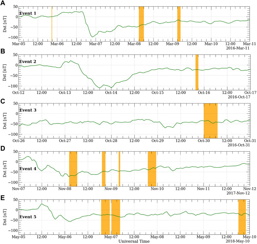
FIGURE 1. The Dst index for the events (A) March 05–10, 2016, (B) October 12–17, 2016, (C) March 26–31, 2016, (D) November 07–12, 2017, and (E) May 05–10, 2018, over CXP.

It is well-known that during magnetic storms, disturbed electric fields can influence the ionosphere through the Prompt Penetration Electric Field (PPEF) (Forbes et al., 1995) or by the Disturbance Dynamo Electric Field (DDEF) (Blanc and Richmond, 1980). However, as shown by Resende et al., (2021), these disturbed electric fields are not capable of causing some influence in the Es layer over CXP. Thus, in this work, we only want to show that the days of the atypical Es layer presence are around the magnetic storm, occurring on both quiet and disturbed days. For this reason, we do not present other interplanetary medium parameters.

Table 1 shows the day of geomagnetic storm onset, the level of the magnetic storm represented by the minimum value reached by the Dst index, the day of the atypical Es layer occurrence, the hour (in universal time), and the condition of the period (quiet or disturbed). The Dst threshold used to classify whether the period is quiet or disturbed is −30 nT. Thus, the days with Dst lower than $-30$ nT are assumed to be disturbed in this study. Here, it is possible to clearly see that the Es layer spreading also occurred in quiet periods. In most cases, the atypical Es layer appears during the recovery magnetic storm phase, which is intriguing since the other Es layer physical formation mechanics also acted in this period. We discuss this behavior later on.

TABLE 1

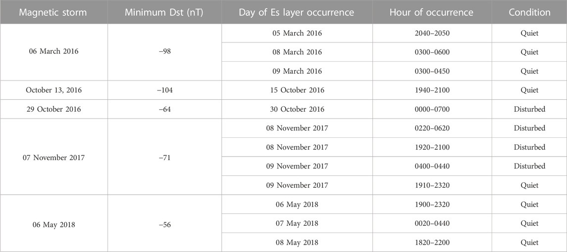
TABLE 1. List of the characteristics of selected events from 2016 to 2018 used in this analysis over CXP. We have the magnetic storm’s day, the Dst minimum, the day of the atypical Es layer occurrence, the hour of their occurrence and the condition of the period.

3.2 The anomalous Es layers occurrence over CXP

The significant modifications in the Es layer electron density distribution occurred in the periods shown in Table 1. Figure 2 shows some ionograms for (a) March 05, (b) March 08, and (c) March 09. The fbEs and the ftEs are shown in vertical black lines. We observe a spread Es layer (red and blue arrows) in all ionograms. The main characteristic here is the low values of the fbEs, which means that the Es layer did not block the F region significantly.

FIGURE 2

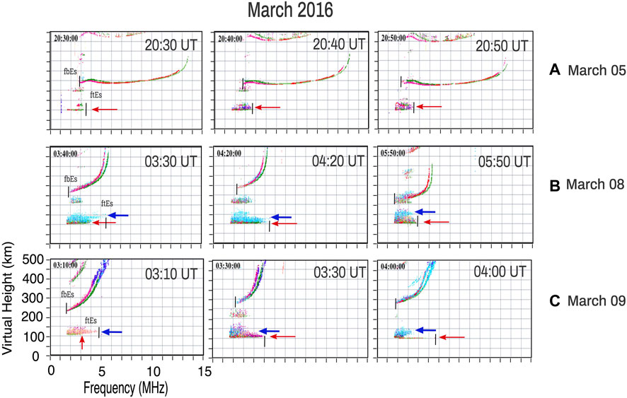
FIGURE 2. Ionograms at CXP (A) from 2030 UT to 2050 UT on 05 March, 2016, (B) collected at hours 0330 UT, 0420 UT, and 0550 UT on 08 March 2016, (C) collected at hours 0310 UT, 0330 UT, and 0400 UT on 09 March 2016.

We believe that the wind shear mechanism is acting in all the Es layer development shown in Figure 2 (represented by red arrows). The background and second reflection trace in ionograms consolidates this statement. On March 05, 2016, an Es layer of the “c” type developed around 115 km beyond the spreading Es layer at 2050 UT. On March 08 and 09, 2016, we noticed a slant Es layer (blue arrow), more expressive at 0330 UT on March 08 and 0400 UT on March 09. This specific type, called “s”, is associated with the gravity waves presence (Cohen et al., 1962).

Another important point is that these events occurred in periods considered quiet times, although March 08 and 09, 2016, are in the recovery magnetic storm phase. In fact, this spread Es layer can be attributed to the Es_a (auroral) layer during the recovery magnetic storm phase. As discussed by Da Silva et al., (2022) and Moro et al., (2022), the particle precipitation mechanism can develop the Es_a layer over the Brazilian sector due to the SAMA presence. The Es_a layer signatures are expected during the recovery magnetic storm phase over Santa Maria and Cachoeira Paulista, which is discussed in the following section.

The same spreading Es layer behavior occurred in the other events. Figure 3 presents some selected ionograms on (a) 15 October 2016, (b) 09 November 2017, and (c) May 08, 2018. In these ionograms, the fbEs also have low values (fbEs $\le$ 3 MHz). The ftEs was lower than 7 MHz. The Es_s presence is also observed over CXP (red arrow).

FIGURE 3

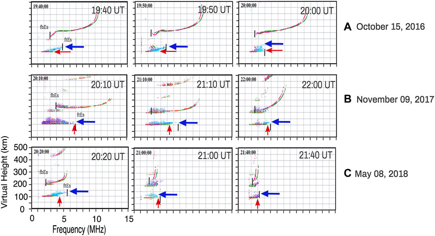
FIGURE 3. Some selected ionograms at CXP for (A) 1940 UT, 1950 UT, and 2000 UT on 15 October 2016, (B) 2010 UT, 2110 UT, and 2200 UT on 09 November 2017, (C) 2020 UT, 2100 UT, and 2140 UT on 08 May 2018.

The other case in which the Es layer over CXP suffered a significant modification was on 30 October 2016. Figure 4 shows the ionogram sequences of these Es layers over CXP between 0330 UT and 0610 UT intervals. We notice that the Es_s is present between 0430 UT and 0450 UT. Also, the ftEs reached values around 7 MHz at 0410 UT. In this specific ionogram, it is plausible that competition is occurring between the Es layer formation mechanisms, such as wind shear, particle precipitation, and instabilities. The following section shows the particle precipitation’s role in these events.

FIGURE 4

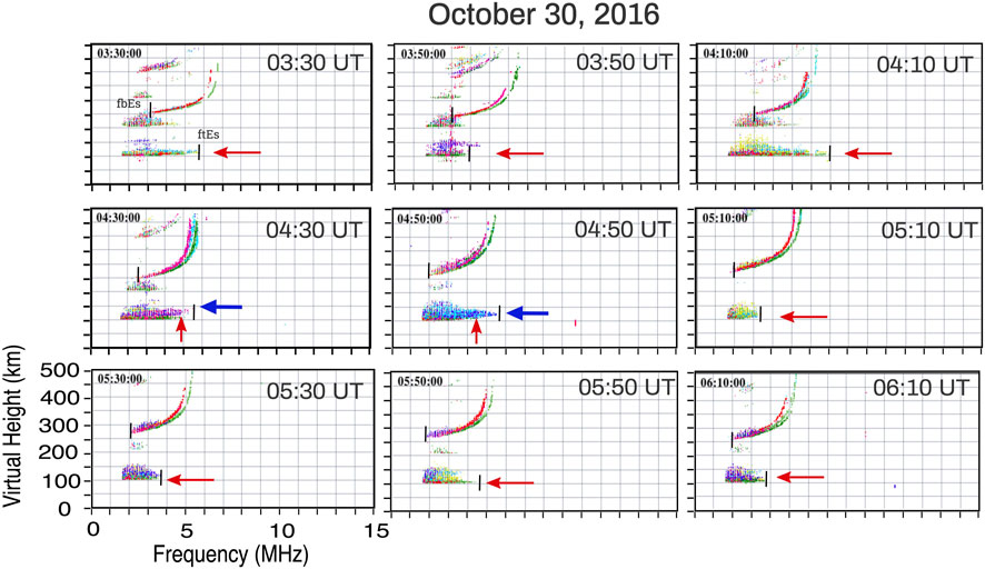
FIGURE 4. Ionograms at CXP from 0330 UT to 06100 UT for each 20 min on 30 October 2016.

3.3 Particle precipitation analysis

The reason that intrigues us about these events is that the spread Es layer has two different characteristics to the auroral trace, such as: (1) the spread occurrence during quiet periods (Dst larger than −30 nT) and (2) the inclination of the trace in some cases, showing the gravity waves presence. Thus, one important step of this work is to discard the particle precipitation mechanism. In this context, we examined the AE index and particle dynamics in the inner radiation belt.

Figure 5 shows the AE index on 08 March 2016, between 2100 UT and 2300 UT (upper -a) and between 0300 UT and 0500 UT (bottom -b) on 09 March 2016, as used as an example. In general, the AE index shows low values in these hours, not reaching 150 nT most of the time. A short period (after 04:00 UT) that the AE was more extensive than 150 nT. This means that the entry of particles into the polar ionosphere and, consequently, their transport toward the low/equatorial ionosphere is not visible in this period. Thus, particle precipitation is an unlikely mechanism in these Es layer development. In other cases of Table 1, the AE is following the same pattern with low values, except on 30 October 2016.

FIGURE 5

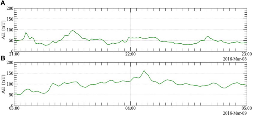
FIGURE 5. AE index on 08 March 2016, between 2100 UT and 2300 UT upper-(A) and between 0300 UT and 0500 UT bottom-(B) on 09 March 2016.

To confirm that these spreading Es layer does not correlate with the particle precipitation, we show Figure 6. In this figure, the Power Spectral Density (PSD) of the magnetic field (Bw) is presented during the short times on March 05, 2016 (panel a), 08 March 2018 (panel b), and March 09 (panel c). We concentrate on the period that the spreading Es layer was observed. Red, yellow, black, and blue lines represent 0.9 fce, 0.5 fce, 0.1 fce, and total electron density, respectively. The purpose is to detect the hiss waves close to the perigee (at the inner radiation belt), that are responsible for causing the particle precipitation into the atmosphere over the SAMA region. This figure shows that the PSD of the hiss waves is considerably low (≤10⁻⁷ nT²/Hz-red arrows) during these three quiet periods. The literature (Da Silva et al., 2022; Moro et al., 2022) shows that the power spectral density of the hiss waves able to cause the low-energy electron precipitation (tens of keV) over the SAMA region is ≥10⁻⁵ nT²/Hz. Therefore, the low PSD of the hiss waves during these quiet periods (<10⁻⁷ nT²/Hz) may not be efficient in causing the low-energy electron precipitation (from 0.5 keV to tens of keV) over the SAMA region. The other cases also presented low values in PSD of the hiss waves (≤10⁻⁷ nT²/Hz) (not shown here).

FIGURE 6

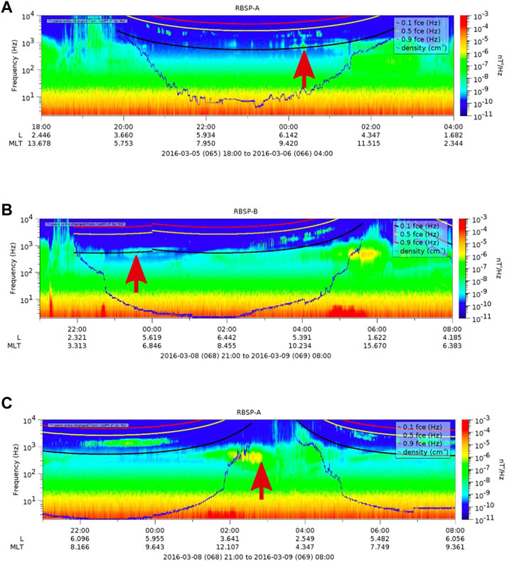
FIGURE 6. Power spectral density of the magnetic field from EMFISIS instrument onboard Van Allen Probes on March 05, 2016 (A), 08 March 2018 (B), and March 09 (C).

The exception occurred on 30 October 2016, in which it is possible to observe that the hiss wave PSD (∼10⁻⁴ nT²/Hz) (Figure 7) is similar to the results discussed by Da Silva et al., (2022). This value is enough to allow low-energy electron precipitation (from 0.5 keV to tens of keV) caused by hiss waves over the SAMA region. In this case, the AE reached values higher than 500 nT. Here, we intend to show that the plasmaspheric hiss waves inside the inner radiation belt reached significant values, and the particle precipitation in the SAMA region can occur in this event.

FIGURE 7

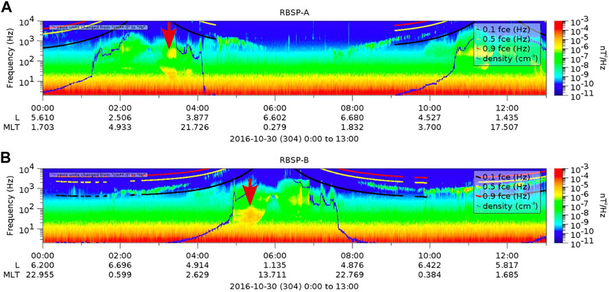
FIGURE 7. Power spectral density of the magnetic field from EMFISIS instrument onboard Van Allen Probe (A) and (B) on 30 October 2016.

Therefore, we proposed here that the spreading Es layer can occur due to other physical mechanisms than particle precipitation due to the SAMA in most cases. Evidence of low values of the power spectral density of the hiss waves and AE index confirms this statement. Additionally, although the event on 30 October 2016, can have particle precipitation influence, we notice the gravity wave presence (Es_s occurrence). Thus, we believe that there are competing physics mechanisms in the Es layer formation in this event.

3.4 The possible instability action in the Es layer development

One of the possibilities of these spreading Es layer occurrences is the instability formation that can affect the wind shear. In other words, the Es layer may be formed initially by wind shear, and the environment becomes unstable due to gravity waves, creating inhomogeneous layers in ionograms. In this context, the Kelvin-Helmholtz instability (KHI) stands out as one of the most classical instabilities in fluid mechanics. These instability billows are triggered by unstable winds or gravity waves (Yan et al., 2021).

Another instability that can occur is Gradient Drift instability (GDI), which has an initial condition, the polarization electric field produced by a Hall current, and the density gradient in the same vertical direction (Rastogi 1972). The GDI is common in equatorial regions, where the Electrojet Equatorial Current (EEJ) presence creates favorable circumstances for their occurrence. Resende et al., (2016) showed the effect of this irregularity in the Es layer over the Brazilian sector. In their results, the authors mentioned that this instability depends on the strong electric field, which is found in the EEJ. Thus, the GDI is responsible for the equatorial Es layer (Es_q) in stations near the magnetic equator.

Although some authors have studied this type of instability at mid-latitudes [see Rosado-Román et al., 2004 and references therein], the GDI effect occurs around sunset because the electric field is stronger (around 3 mV/m). However, the layers associated with this irregularity were only observed in data from radar and rockets and did not last long. Resende et al., (2021) mention that the electric field does not influence the Es layer behavior over Cachoeira Paulista. For this reason, we believe that the most probable mechanism that acted in the atypical Es layer is the KHI.

The first evidence of the instabilities in the ionospheric plasma is the low values of the fbEs, meaning that the upper region above the Es layer has not been blocked. Table 2 shows the difference between the ftEs and fbEs (ftEs-fbEs) during the spreading Es layer occurrence. We present the maximum and minimum differences within the period studied.

TABLE 2

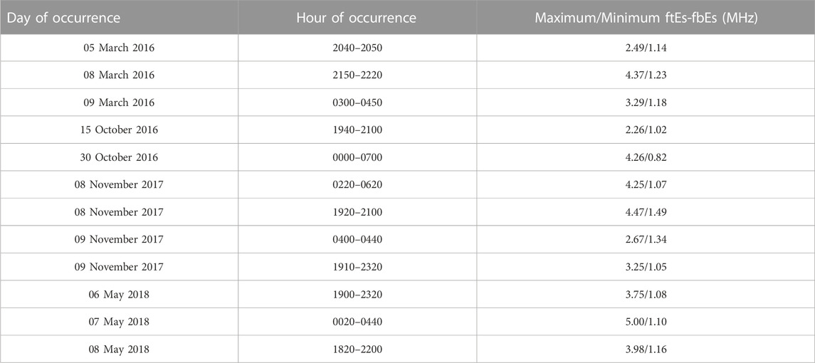
TABLE 2. Maximum and minimum differences of the ftEs and fbEs parameters of the period shown in Table 1.

In general, the differences between the frequency parameters show that the winds have a secondary role in the Es layer development in most cases. The low values of the ftEs-fbEs mean that the upper region is blocked. On the other hands, the high values of these differences mean that the Es layers have not blocked the upper layer. Thus, the wind shear that is the main mechanism to form denser layers could be stronger in such hours. The Es layer can be also formed by other mechanisms such as instabilities, particle precipitation, and gravity waves. However, the Es layers formed by these other mechanisms do not absorb the digosonde signal, from upper ionosphere layers, as those denser layers formed by wind shear. This is an indication that irregularities can be present. The minimum values of the ftEs-fbEs observed in our events analyzed here were higher than 1, except on 30 October 2018. Therefore, our results showed an indication that the unstable Es layer in the ionograms profile over CXP can be due to the instabilities since the particle precipitation seems to have influenced only the event on 30 October 2018.

The instability due to the winds or gravity waves is the most probable cause of this unusual Es layer behavior. We used the SKiYMET data for zonal and meridional winds to analyze if the winds were unstable. The wind measurements were interpolated to obtain a sample interval of 1 min. Afterward, we obtained the energy spectrum E(k) through Fourier transformation. Hence, we verified whether the result follows the −5/3 Kolmogorov spectrum prediction for turbulent flows. If this behavior happens, the winds are considered turbulent. All the details about the Kolmogorov technique are given by Calif et al., (2016).

Figure 8 shows the previous analysis results using the SKiYMET data for the zonal (right) and meridional (left) wind components on March 05–06, 2016, and October 29–30, 2016 (blue line). We choose the height of 99 km, which is the typical altitude of the Es layer occurrence. We also compared the results to the −5/3 Kolmogorov spectrum, plotted in orange in these graphs. The wind speed sampling step is 1 h due to the limitations of the technique and equipment used to obtain the data. We interpolated the values using a cubic spline to 1 min to.

1. Use the existing, validated FFT algorithms available;

2. Fill minor gaps in the data; and

3. Slightly smooth the output due to the signal characteristics.

FIGURE 8

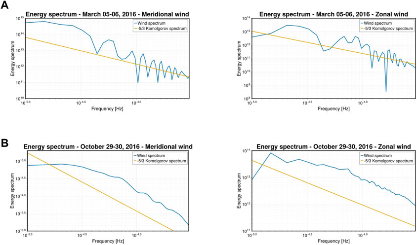
FIGURE 8. The Fourier power spectral densities of the SKiYMET data for the meridional (upper) and zonal (below) components on March 05–06, 2016 (A), and October 29–30, 2016 (B), in the blue line. The −5/3 Kolmogorov spectrum given in the orange line in these graphs.

Although this procedure can change the spectrum in higher frequencies, we analyzed only the frequencies up to 10^(−3.5) Hz. This region corresponds to periods of roughly 1 h, which matches the equipment sampling rate. Hence, the interpolation used in this work does not significantly modify the spectrum in the region we are interested in.

The wind components spectra demonstrate an unstable behavior for the frequencies between 10⁻⁵ and 10⁻⁴ on March 05–06, 2016, as seen in Figure 8. Notice that this result was found close to the −5/3 Kolmogorov value. This fact means that the wind is turbulent at this height during this period. However, in the specific case of October 29–30, 2016, the components of the winds are not oscillating, and the power spectral density is not so close to the −5/3 Kolmogorov value. In other words, the wind does not appear to be turbulent.

This analysis provides clear evidence that the spreading Es layer over a low latitude station can occur due to the instabilities. The most probable is the KHI, which is driven by shear flow and is common in the atmosphere (Ecklund et al., 1981; Chen et al., 2020). Using simulations, Wu et al., (2022) analyzed the KHI in the middle and low Es layers. The simulations presented multiple striation structures in the Es layer. The authors found that the polarization electric field is induced in the horizontal structure of the sporadic E (Es) layer, and it is an initial condition to grow up the KHI or GDI.

The KHI mechanism in the Es layer development, mainly in the low latitude regions, has not been widely studied yet. Bernhardt (2002) studied the KHI effect driven by wind shear to explain the unstable structures in the Es layer. They used coupled models of the irregularities generated by sheared neutral winds and KHI billows in the Es layer between 100–120 km. The simulations indicated that the KHI could significantly impact the sporadic-E layer structures. Additionally, Bernhardt (2002) concluded that a complex evolution of the Es layer from the KHI and other improvements in the model is necessary to answer the real instability role in developing these unstable Es layers.

Liu et al., (2022) analyze the Es layer behavior using the Digisonde data applying a technique called frequency domain interferometry (FDI) over Wuhan, China (114°E, 30°N). The FDI allowed them to observe the inhomogeneous Es layer occurrence in such station. The complex structure of the Es layer found by the authors can be associated with instability or gravity wave modulation. One plausible explanation is the KHI presence in the Es layer formation that is caused by the strong shear of the neutral background wind.

Several authors mentioned that gravity waves could trigger the instabilities besides the winds. Unfortunately, the airglow images are restricted to clear skies. Therefore, among the analyzed events, only one presents good images. Figure 9 shows the OH images on 06 May 2018, at 2315 UT (panel a). The white square with red arrows means the gravity waves presence. In fact, we observed the clear gravity wave propagation for the entire night on May 06 and 07, 2018. Panel b of Figure 9 shows the Es_s layer presence in ionograms during the nighttime when we observe the gravity waves in imager data.

FIGURE 9

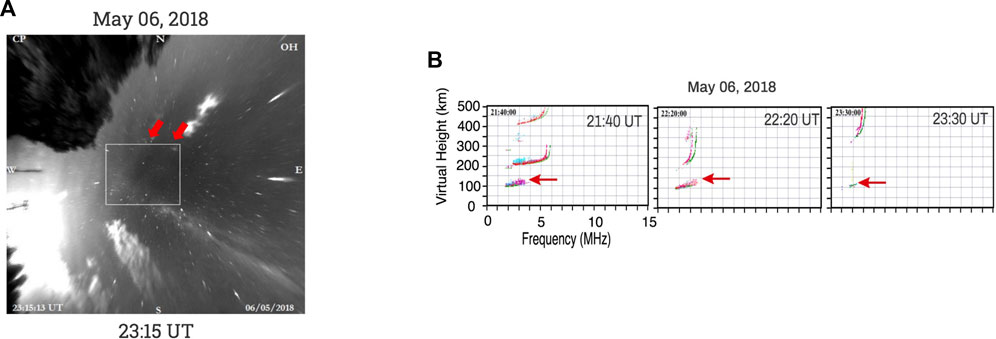
FIGURE 9. The OH images showing the gravity waves presence at 2315 UT on 06 May 2018 (A), and the Es_s layer in ionograms (B) in the nighttime period on 06 May 2018.

The Es_s is associated with the gravity wave mechanism, and it is characterized by a trace that grows continuously in frequency and emerges from another type of Es trace, as shown in red arrows. This specific Es layer type is not common in the Brazilian sector, as shown in Conceição-Santos et al., (2019) and Moro et al., (2022). We notice that the Es_s layer was observed in some hours for all events mentioned in Table 1. Thus, there is a possibility that the gravity waves may have a precursor to the growth of instability.

Therefore, an important discovery of this work is that the spreading Es layer, mainly during quiet times, is not necessarily due to the particle precipitation due to the SAMA presence. We found that the wind shear can be turbulent, influencing the Es layer development. Lastly, further research is necessary to affirm what is the exact instability that acts on the Es layer formation.

4 Conclusion

We study the atypical and spreading Es layer over CXP in days before, during, and after the magnetic storms from 2016 to 2018. We analyzed the Digisonde data, imager, satellite, and meteor radar to understand the dynamic formation processes of these inhomogeneous Es layers.

The significant modifications in the Es layer electron density distribution were observed in ionograms on days before and after the magnetic storm. The main characteristic is the low values of the fbEs, which means that the Es layer does not block the F region significantly. In fact, the high difference between the ftEs and fbEs (ftEs-fbEs) during the spreading Es layer occurrence indicated that the irregularities could be present.

The inhomogeneous Es layer is associated with the Es_a layer over CXP due to SAMA. However, we also observe that the spreading Es layers occurred in days before the magnetic storms or quiet times. We examined the AE index and particle dynamics in the inner radiation belt to discard the particle precipitation mechanism. Our results showed a low power spectral density of the hiss waves in these events (<10⁻⁷ nT²/Hz), inefficiently causing electron precipitation over the SAMA region.

The exception was on 30 October 2016. In this case, the spreading Es layer occurred in hours when AE was higher than 500 nT. Also, the power spectral density of the hiss waves was ∼10⁻⁴ nT²/Hz, similar to the previous studies about the Es_a layer formation. Therefore, this value is enough to cause low-energy electron precipitation (from 0.5 keV to tens of keV) by hiss waves over the SAMA region.

One of the possibilities of these spreading Es layer occurrences is the instability formation that can affect the wind shear. In other words, the Es layer may be formed initially by wind shear, and the environment becomes unstable due to the electric field or gravity waves, creating inhomogeneous layers in ionograms. We used the SKiYMET data for zonal and meridional winds to analyze if the winds were unstable. The temporal resolution of these wind data is 1 h. As no other wind data is available, a linear interpolation was performed every minute to visualize whether the wind could have turbulence. The analysis is not so impaired as we only use measurements between 80 and 100 km.

Using these winds data, we compute energy spectrum E(k) to verify the turbulence in the winds. In fact, we analyzed whether the power spectral densities are close to the −5/3 Kolmogorov spectrum. In almost all events, the wind components spectra were close to the −5/3 Kolmogorov value. This fact means that the wind is turbulent. However, in the specific case of 30 October 2016, the wind energy spectrum components were not oscillating, and the power spectral density is not so close to the −5/3 Kolmogorov value.

The spreading Es layer observed in our data has an inclined trace in some hours, the Es_s layer. This Es layer type is associated with the gravity wave mechanism. Several authors mentioned that gravity waves could trigger the instabilities besides the winds. The OH emission in airglow images shows a gravity wave propagation on May 06 and 07, 2018. At the same hours, we observe the Es_s layer presence in ionograms. Thus, the presence of gravity waves may have been a trigger for the instability occurrence.

Finally, an important discovery of this work is that the spreading Es layer, mainly during quiet times, is not necessarily formed by the particle precipitation due to the SAMA. We found that the wind shear can be turbulent, influencing the Es layer development and contributing significantly to our understanding of the different mechanism actions in the atypical Es layer. However, further research is necessary to conclude precisely what instability caused these inhomogeneous Es layers over CXP.

Data availability statement

The datasets presented in this study can be found in online repositories. The names of the repository/repositories and accession number(s) can be found below: http://www2.inpe.br/climaespacial/portal/en/.

Author contributions

LR, YZ, CD, and LD contributed to the conception and design of the study. LR, VA, LD, and CF organized the database. JM and SC analyzed the interplanetary medium conditions and magnetospheric conditions. LR, JM, RS, SC, CW, HL, ZL, and CF interpreted the ionospheric data. RC help in the mathematical tools. LR, LD, and JM analyzed the Atmospheric ionization over SAMA. LR wrote the first draft of the manuscript. All authors contributed to the article and approved the submitted version.

Funding

This research was also supported by the National Natural Science Foundation of China (42074201 and 41674145), by the International Partnership Program of Chinese Academy of Sciences (grants 183311KYSB20200003 and 183311KYSB20200017).

Acknowledgments

LR would like to thank the China-Brazil Joint Laboratory for Space Weather (CBJLSW), National Space Science Center (NSSC), Chinese Academy of Sciences (CAS) for supporting her postdoctoral. CD thanks CNPq/MCTI, grant 03121/2014-9. SC and RS thanks CNPq/MCTI (grants 303643/2017-0 and 300849/2023-0). VA, LD, and JM would like to thank the CBJLSW/NSSC/CAS for supporting their postdoctoral. SC thanks CAPES/MEC (grant 88887.362982/2019-00). The authors thank the OMNIWEB for providing AE and Dst parameters used in the classification of the days. The Digisonde data from Cachoeira Paulista, imager data, and wind data can be downloaded upon registration at the Embrace webpage from INPE Space Weather Program in the following link: http://www2.inpe.br/climaespacial/portal/en/.

Conflict of interest

The authors declare that the research was conducted in the absence of any commercial or financial relationships that could be construed as a potential conflict of interest.

Publisher’s note

All claims expressed in this article are solely those of the authors and do not necessarily represent those of their affiliated organizations, or those of the publisher, the editors and the reviewers. Any product that may be evaluated in this article, or claim that may be made by its manufacturer, is not guaranteed or endorsed by the publisher.

References

Bernhardt, P. A. (2002). The modulation of sporadic-E layers by Kelvin–Helmholtz billows in the neutral atmosphere. J. Atmos. Solar-Terrestrial Phys. 64 (12-14), 1487–1504. doi:10.1016/S1364-6826(02)00086-X

CrossRef Full Text | Google Scholar

Blanc, M., and Richmond, A. D. (1980). The ionospheric disturbance dynamo. J. Geophys. Res. Space Phys. 85 (4), 1669–1686. doi:10.1029/JA085iA04p01669

CrossRef Full Text | Google Scholar

Calif, R., Schmitt, F., and Medina, O. (2016). “−5/3 Kolmogorov turbulent behavior and intermittent sustainable energies,” in Sustainable energy - technological issues, applications and case studies (London, UK: Intechopen). doi:10.5772/106341

CrossRef Full Text | Google Scholar

Chen, G., Wang, Z., Jin, H., Yan, C., Zhang, S., Feng, J., et al. (2020). A case study of the daytime intense radar backscatter and strong ionospheric scintillation related to the low-latitude E-region irregularities. J. Geophys. Res. Space Phys. 125, e2019JA027532. doi:10.1029/2019JA027532

CrossRef Full Text | Google Scholar

Cohen, R., Calvert, W., and Bowles, K. L. (1962). On the nature of equatorial slant sporadicE. J. Geophys. Res. Space Phys. 67, 965–972. doi:10.1029/JZ067i003p00965

CrossRef Full Text | Google Scholar

Conceição-Santos, F., Muella, M. T. A. H., Resende, L. C. A., Fagundes, P. R., Andrioli, V. F., Batista, P. P., et al. (2019). Occurrence and modeling examination of sporadic-E layers in the region of the south America (atlantic) magnetic anomaly. J. Geophys. Res. Space Phys. 124 (11), 9676–9694. doi:10.1029/2018JA026397

CrossRef Full Text | Google Scholar

Da Silva, L. A., Shi, J., Resende, L. C. A., Agapitov, O. V., AlvesBatistaArras, L. R. I. S. C., Vieira, L. E., et al. (2022). High-energy electron flux enhancement pattern in the outer radiation belt in response to the alfvénic fluctuations within high-speed solar wind stream: A statistical analysis. J. Geophys. Research-Space Phys. 126. doi:10.1029/2021ja029363

CrossRef Full Text | Google Scholar

Dagar, R., Verma, P., Napgal, O. P., and Setty, C. S. G. K. (1977). The relative effects of the electric fields and neutral winds on the formation of the equatorial sporadic layers. Ann. Geophys. 33 (3), 333–340.

Google Scholar

Ecklund, W. L., Carter, D. A., and Balsley, B. B. (1981). Gradient drift irregularities in mid-latitude sporadicE. J. Geophys. Res. Space Phys. 88 (2), 858–862. doi:10.1029/JA086iA02p00858

CrossRef Full Text | Google Scholar

Forbes, J. M., Roble, R. G., and Marcos, F. A. (1995). Equatorial penetration of magnetic disturbance effects in the thermosphere and ionosphere. J. Atmos. Terr. Phys. 57 (10), 1085–1093. doi:10.1016/0021-9169(94)00124-7

CrossRef Full Text | Google Scholar

Haldoupis, C. (2011). A tutorial review on sporadic E layers. IAGA Book Ser. 29 (2), 381–394. doi:10.1007/978-94-007-0326-1_29

CrossRef Full Text | Google Scholar

Hocking, W. K., Fuller, B., and Vandepeer, B. (2001). Real-time determination of meteorrelated parameters utilizing modern digital technology. J. Atmos. Terr. Phys. 63 (2-3), 155–169. doi:10.1016/S1364-6826(00)00138-3

CrossRef Full Text | Google Scholar

Hocking, W. K., and Thayaparan, T. (1997). Simultaneous and colocated observation of winds and tides by MF and meteor radars over London, Canada (43°N, 81°W), during 1994-1996. Radio Sci. 32, 833–865. doi:10.1029/96RS03467

CrossRef Full Text | Google Scholar

Kletzing, C. A., Kurth, W. S., Acuna, M., MacDowall, R. J., Torbert, R. B., Averkamp, T., et al. (2013). The electric and magnetic field instrument suite and integrated science (EMFISIS) on RBSP. Space Sci. Rev. 179 (1–4), 127–181. doi:10.1007/s11214-013-9993-6

CrossRef Full Text | Google Scholar

Kopp, E. (1997). On the abundance of metal ions in the lower ionosphere. J. Geophys. Res. Space Phys. 102, 9667–9674. doi:10.1029/97ja00384

CrossRef Full Text | Google Scholar

Kumar, D. V. P., Patra, A. K., Kwark, Y. S., Kim, K. H., and Yellaiah, G. (2009). Low latitude E-region irregularities studied using Gadanki radar, ionosonde and in situ measured electron density. Astrophysics Space Sci. 323, 225–233. doi:10.1007/s10509-009-0066-y

CrossRef Full Text | Google Scholar

Liu, T., Yang, G., Zhou, C., Jiang, C., Xu, W., Ni, B., et al. (2022). Improved ionosonde monitoring of the sporadic E layer using the frequency domain interferometry technique. Remote Sens. 14, 1915. doi:10.3390/rs14081915

CrossRef Full Text | Google Scholar

Mathews, J. D. (1998). Sporadic E: Current views and recent progress. J. Atmos. Terr. Phys. 60, 413–435. doi:10.1016/S1364-6826(97)00043-6

CrossRef Full Text | Google Scholar

Matsushita, S., and Reddy, C. A. (1967). A study of blanketing sporadic E at middle latitudes. J. Geophys. Res. Space Phys. 72 (11), 2903–2916. doi:10.1029/JZ072i011p02903

CrossRef Full Text | Google Scholar

Mauk, B. H., Fox, N. J., Kanekal, S. G., Kessel, R. L., Sibeck, D. G., and Ukhorskiy, A. (2012). Science objectives and rationale for the radiation belt storm probes mission. Space Sci. Rev. 179, 3–27. doi:10.1007/s11214-012-9908-y

CrossRef Full Text | Google Scholar

Medeiros, A. F., Buriti, R. A., Machado, E. A., Takahashi, H., Batista, P. P., Gobbi, D., et al. (2004). Comparison of gravity wave activity observed by airglow imaging at two different latitudes in Brazil. J. Atmos. Solar-Terrestrial Phys. 66 (6-9), 647–654. doi:10.1016/j.jastp.2004.01.016

CrossRef Full Text | Google Scholar

Moro, J., Xu, J., Denardini, C. M., Resende, L. C. A., Da Silva, L. A., Chen, S. S., et al. (2022). Different sporadic-E (Es) layer types development during the august 2018 geomagnetic storm: Evidence of auroral type (Esa) over the SAMA region. J. Geophys. Res. Space Phys. 127, e2021JA029701. doi:10.1029/2021JA029701

CrossRef Full Text | Google Scholar

Rastogi, R. G. (1972). Equatorial sporadic E and plasma instabilities. Nature 237, 73–75. doi:10.1038/physci237073b0

CrossRef Full Text | Google Scholar

Reinisch, B. W., Galkin, I. A., Khmyrov, G. M., Kozlov, A., and Kitrosser, D. (2004). Automated collection and dissemination of ionospheric data from the Digisonde network. Adv. Radio Sci. 2, 241–247. doi:10.5194/ars-2-241-2004

CrossRef Full Text | Google Scholar

Resende, L. C. A., Batista, I. S., Denardini, C. M., Batista, P. P., Carrasco, A. J., Andrioli, V. F., et al. (2017). Simulations of blanketing sporadic E-layer over the Brazilian sector driven by tidal winds. J. Atmos. Solar-Terrestrial Phys. 154, 104–114. doi:10.1016/j.jastp.2016.12.012

CrossRef Full Text | Google Scholar

Resende, L. C. A., Batista, I. S., Denardini, C. M., Carrasco, A. J., Andrioli, V. F., Moro, J., et al. (2016). Competition between winds and electric fields in the formation of blanketing sporadic E layers at equatorial regions. Earth Planets Space 68, 201. doi:10.1186/s40623-016-0577-z

CrossRef Full Text | Google Scholar

Resende, L. C. A., Denardini, C. M., and Batista, I. S. (2013). Abnormal fbEs enhancements in equatorial Es layers during magnetic storms of solar cycle 23. J. Atmos. Solar-Terrestrial Phys. 102, 228–234. doi:10.1016/j.jastp.2013.05.020

CrossRef Full Text | Google Scholar

Resende, L. C. A., J Shi, J. K., Denardini, C. M., Batista, I. S., Picanço, G. A., Moro, J., et al. (2021). The impact of the disturbed electric field in the sporadic E (Es) layer development over Brazilian region. J. Geophys. Res. Space Phys. 126, e2020JA028598. doi:10.1029/2020JA028598

CrossRef Full Text | Google Scholar

Resende, L. C. A., Zhu, Y., Denardini, C. M., Moro, J., Arras, C., Chagas, R. A. J., et al. (2022). Worldwide study of the Sporadic E (Es) layer development during a space weather event. J. Atmos. Solar-Terrestrial Phys. 241, 105966. doi:10.1016/j.jastp.2022.105966

CrossRef Full Text | Google Scholar

Resende, L. C. A., Shi, J. K., Denardini, C. M., Batista, I. S., Nogueira, P. A. B., Arras, C., Andrioli, V. F., Moro, J., et al. (2020). The influence of disturbance dynamo electric field in the formation of strong sporadic E-layers over Boa Vista, a low latitude station in American Sector. J. Geophys. Res. Space Phys. 108 (5), 1176. doi:10.1029/2019JA027519

CrossRef Full Text | Google Scholar

Rosado-Román, J. M., Swartz, W. E., and Farley, D. T. (2004). Plasma instabilities observed in the E region over Arecibo and a proposed nonlocal theory. J. Atmos. Solar-Terrestrial Phys. 66 (17), 1593–1602. doi:10.1016/j.jastp.2004.07.005

CrossRef Full Text | Google Scholar

Whitehead, J. (1961). The formation of the sporadic-E layer in the temperate zones. J. Atmos. Terr. Phys. 20 (1), 49–58. doi:10.1016/0021-9169(61)90097-6

CrossRef Full Text | Google Scholar

Wu, J., Zhou, C., Wang, G., Liu, Y., Jiang, C., and Zhao, Z. (2022). Simulation of Es layer modulated by nonlinear Kelvin–Helmholtz instability. J. Geophys. Res. Space Phys. 127, e2021JA030065. doi:10.1029/2021JA030065

CrossRef Full Text | Google Scholar

Yan, C., Chen, G., Wang, Z., Zhang, M., Zhang, S., Li, Y., et al. (2021). Statistical characteristics of the low-latitude E-region irregularities observed by the HCOPAR in south China. J. Geophys. Res. Space Phys. 126, e2021JA029972. doi:10.1029/2021JA029972

CrossRef Full Text | Google Scholar