 Sabrina Carpy
 Maï Bordiec†
 Olivier Bourgeois
- Laboratoire de Planétologie et Géosciences, Centre National de la Recherche Scientifique (UMR6112), Nantes Université, Université d'Angers, Le Mans Université, Nantes, France
Ablation waves involve solid substrate such as ice or soluble rocks. Ablation by sublimation or dissolution under turbulent winds or liquid flows may lead to the development of transverse linear bedforms (ablation waves) on volatile or soluble susbtrates. In glaciology, geomorphology, karstology and planetology, these ablation waves may provide relevant morphological markers to constrain the flows that control their formation. For that purpose, we describe a unified model, that couples mass transfers and turbulent flow dynamics and takes into account the relationship between the viscosity of the fluid and the diffusivity of the ablated material, for both sublimation and dissolution waves. From the stability analysis of the model, we derive three scaling laws that relate the wavelength, the migration velocity and the growth time of the waves to the physical characteristics (pressure, temperature, friction velocity, viscous length, ablation rate) of their environment through coefficients obtained numerically. The laws are validated on terrestrial examples and laboratory experiments of sublimation and dissolution waves. Then, these laws are plotted in specific charts for dissolution waves in liquid water, for sublimation waves in N2-rich atmospheres (e.g., Earth, Titan, Pluto) and in CO2-rich atmospheres (e.g., Mars, Venus). They are applied to rock dissolution on the walls of a limestone cave (Saint-Marcel d’Ardèche, France), to H2O ice sublimation on the North Polar Cap (Mars) and to CH4 ice sublimation in Sputnik Planitia (Pluto), to demonstrate how they can be used (1) either to derive physical conditions on planetary surfaces from observed geometric characteristics of ablation waves (2) or, conversely, to predict geometric characteristics of ablation waves from measured or inferred physical conditions on planetary surfaces. The migration of sublimation waves on regions of the Martian North Polar Cap and sublimation waves candidates on Pluto are discussed.
1 Introduction
Because there is a large occurrence of volatile ices in the Solar System, mass transfers by sublimation and condensation are likely to shape planetary landforms (Law and Van Dijk, 1994; Kreslavsky and Head, 2002a; Byrne and Ingersoll, 2003; Hagedorn et al., 2007; Mangold, 2011). This kind of mass transfers are effective on the Martian North Polar Cap (MNPC), whose spiral troughs and sedimentation waves have been proposed to be the result of sublimation and condensation, enhanced by the wind (Smith et al., 2013; Herny et al., 2014). While these landforms are remarkable for their size, there are many other smaller landforms like suncups giving the MNPC an overall texture of humps and hollows (Malin and Edgett, 2001; Milkovich, 2006; Banks et al., 2010; Massé et al., 2010; Nguyen et al., 2020). For all these landforms, the main processes involved in their generation are associated with phase changes enhanced by the wind (Howard, 2000) leading to a wind-driven redistribution of surface materials (ice, dust) by condensation (James, 1982; Jakosky, 1985; Fanale et al., 1992) and/or by sublimation (Ivanov and Muhleman, 2000; Ng and Zuber, 2006; Smith and Holt, 2010; Massé et al., 2012; Herny et al., 2014). On Pluto (Moores et al., 2017; Moore et al., 2018), the Bladed Terrain Deposits (BTDs) of CH4 currently undergoing sublimation (Bertrand et al., 2019) seems to be sculpted in regular patterns by aeolian processes. On Sputnik Planitia plain, abundant sublimation pits have been observed (Moore et al., 2017) in areas where the wind seems to be weak (Bertrand et al., 2020) while linear and regularly spaced crests primarily composed of CH4-ice (Telfer et al., 2018) has been revealed in the western region of the plain subject to stronger winds (Bertrand et al., 2020). On Earth, the pressure, temperature and humidity conditions required to allow the sublimation of icy surfaces are only found in a few specific locations. These conditions exist on some tropical glaciers at high altitude during the dry season (Winkler et al., 2009), in the Blue Ice Areas (BIAs) in Antarctica (van den Broeke and Bintanja, 1995) and in some ice caves (Curl, 1966; Obleitner and Spötl, 2011). The paucity of terrestrial observations may be why sublimation redistribution processes under turbulent wind have been poorly studied until the area of planetary space exploration.
Among the patterns generated by sublimation, we are interested in transverse linear bedforms, which are periodic ridges perpendicular to the turbulent wind. Bordiec et al. (2020) shows that sublimation waves: (1) can exist at different scales, depending on the environments and climates in which they develop; (2) can be used as morphological markers of surface-atmosphere interactions as are sand dunes (Courrech du Pont et al., 2014) thanks to scaling laws. The observation of these sublimation waves on planetary surfaces makes it possible to constrain or at least define certain characteristics of the environment: (i) the first law gives the wavelength as a function of the velocity of the flow and its viscosity; (ii) the second law links the erosion rate of the icy substrate to the migration velocity of the bedforms; (iii) the third law relates the growth time to the erosion rate and the wavelength. However, only the first law has been validated on terrestrial natural exemples (Bintanja, 1999; Obleitner and Spötl, 2011) and CO2-ice sublimating experiment in our previous study (Bordiec et al., 2020). We are now looking for new terrestrial field analogues or laboratory experiments to assess the validity of our model in the prediction of the erosion rate. This validation step is necessary for the use of these ablation waves as morphological markers before interpreting the observations on other bodies of the Solar System.
For that purpose, we investigate other solid substrates over which bedforms developed under turbulent flows, coupled with mass transfers. Dissolving soluble rocks are good candidates: among dissolution bedforms (Allen, 1971; Meakin and Jamtveit, 2010), we identify dissolution waves refered to as fluted scallops, flutes, or solution ripples in karstology. Dissolution waves formed on a solid substrate are regularly spaced and parallel ridges, oriented perpendicular to the flow (Ford and Williams, 1989; Ginés et al., 2009), and are slightly asymmetrical in cross-section (Blumberg and Curl, 1974; Hammer et al., 2011). They appear in limestone caves (Curl, 1966; Allen, 1971; Goodchild and Ford, 1972) and their wavelength range varies from a few centimeters to several meters. They can be reproduced experimentally on soluble materials such as platinum (Thorness and Hanratty, 1979) and plaster (Blumberg and Curl, 1974). They are used in karstology to predict flow velocity and direction (Blumberg and Curl, 1974).
Thomas (1979) has compiled various examples of occurrences of bedforms on different solid substrates submitted to ablation processes by mass transfer interacting with a turbulent flow. The shapes described seem for the most part to remain independent of the substrate and the ablation and accumulation process, suggesting that the complexity associated with the chemistry of dissolution or the physics of sublimation plays only a secondary role on the final shape of these objects, possibly controlled by the hydrodynamic conditions. We seek to show that an analogy can be established between these two categories of ablation waves with similarity laws. This effort would help to complement the data set of sublimation waves with dissolution waves in order to use ablation waves as morphological markers. To that end, we combine the instability mechanism proposed by Claudin et al. (2017) for dissolution and that proposed by Bordiec et al. (2020) for sublimation. The coefficients of the scaling laws of the latter are recalculated as a function of the type of ablation (dissolution/sublimation) taking into account the viscosity of the fluid and the diffusivity of the ablated material through the Schmidt number.
A review of observations and experimental measurements are presented for sublimation waves in §2 and dissolution waves in §3. We propose new scaling laws derived from the unified model validated on previous examples in §4. In §5, the laws are plotted in a family of curves enabling to simplify the computations in different environmental conditions: (i) for planetary applications, depending on the pressure and temperature ranges of each planetary body likely to present sublimation waves at its surface and (ii) for dissolution waves in liquid water. In particular, the migration of the sublimation waves of regions of the North Polar Cap of Mars and the case of sublimation waves candidates on Pluto will be discussed. The feasibility of new experiments in terms of growth time and scale could be evaluated using the charts designed for this purpose.
2 Sublimation waves on volatile ices
Space exploration confirmed the presence of volatile ice, either water ice or ice of different compositions on many other bodies in the Solar System (Figure 1). Apart from the Earth where water is in a liquid state on its surface and evaporates, the most efficient phase transition in the Solar System is sublimation which allows ice to transform directly into vapor. In environments favorable to sublimation enhanced by the wind, a wide variety of solid bedforms, differing both in shape and size are observed. In this section, we identify the bodies in the Solar System for which the environmental conditions are favorable for the generation of sublimation waves and collect morphological and physical characteristics representative of each environment.
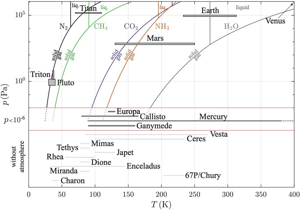
FIGURE 1. Superimposed phase diagrams of the mainly volatiles species (N2, CH4, CO2, NH3, H2O) in the Solar System in (p, T) space, from the Clausius-Clapeyron relation. The mean pressure and temperature conditions of planetary bodies likely to host ice are plotted (on average, shaded areas). The upper part of the figure corresponds to bodies with an atmosphere p >10–2 Pa. The lower part (p <10–6 Pa) contains bodies with little or no atmosphere. Vapour pressure of a species has to be compared to the saturation vapour pressure to determine if sublimation/condensation occur.
2.1 Volatile substrates revealed by space exploration
2.1.1 Inner Solar System
Detection of ice on Mercury is confirmed by surface reflectance measurements combined with images acquired aboard MESSENGER spacecraft. Given its small size and proximity to the Sun, the planet does not have an atmosphere and therefore has extreme temperatures at its surface (from 90 to 700 K), which do not allow ice to exist, with the exception of water ice in the permanently shaded polar regions (Eke et al., 2017). Water ice also exists on the floor of some craters and in cold micro-traps (Deutsch et al., 2017), the origin of which would come from recent impacts (Ernst et al., 2018).
On Venus, the almost exclusive composition of its thick atmosphere in CO2 creates a greenhouse effect such that the temperature of its surface is on the order of 740 K, which makes impossible the presence of ice, whatever its nature, on its surface. Nevertheless there could be an exotic solid substrate deposit: the radar anomalies (high reflectance) linked to the presence of heavy metals (Port et al., 2020), and their deposition in the form of frost (Schaefer and Fegley, 2004) could be enhanced by the aeolian processes proposed on Venus (Kreslavsly and Bondarenko, 2017).
Water ice (seasonal snow, permafrost, pack ice, glaciers) is present in abundance on Earth (Ohmura, 2004) and the atmosphere allows to maintain stable conditions for water ice. The other gases in the atmosphere are unlikely to condense, given their phase diagrams (CO2 and NH3).
Instruments aboard the Lunar Reconnaissance Orbiter (LRO) spacecraft are locating and quantifying water ice on the Moon. Like Mercury, there is no atmosphere and its surface is subject to extreme temperatures and some deep polar cold traps (≃ 3.5%), which never see the Sun’s rays, have exposed ice, in a mixture of ice and regolith (Li et al., 2018).
Among the many martian missions, the Mars Global Surveyor (MGS) and Mars Reconnaissance Orbiter (MRO) missions, and more recently the Trace Gas Orbiter of the ExoMars mission, are providing comprehensive information about the planet’s surface and atmosphere. Currently, the thin atmosphere of Mars composed mainly of CO2 and its distance from the Sun make it a cold planet, well below the solidification point of water, and cold enough to condense CO2. Mars has two imposing polar caps mainly made up of water ice covered with CO2 ice, seasonally for the North, and perennially for the South (Kieffer et al., 1976; James, 1982; Kelly et al., 2007; Byrne, 2009), and there are many other ice reservoirs on its surface outside the poles. Mounds of water ice has been observed on the floor of the deepest craters in the North Polar region (Conway et al., 2012) and the South Polar region (Sori et al., 2019), in which a specific and favorable microclimate allows the accumulation of ice. Moreover, underground ice, more or less covered with dust, exists on nearly a third of the Martian surface (Baker, 2001; Kreslavsky and Head, 2002b).
2.1.2 Outer Solar System
The asteroids Vesta and Ceres have been explored by the Dawn mission. The presence of water ice has been suggested at the north pole of Vesta (Stubbs and Wang, 2012; Scully et al., 2015) and assumed for Ceres from its density and shape (Carroll, 2019).
Galileo is currently the only spacecraft to have orbited Jupiter. In 2023, the ESA mission JUICE flies over and will take a closer look at the three moons Europa, Ganymede and Callisto. It will be followed by Europa Clipper, which will probe the ocean beneath Europa’s ice crust. These moons are covered by a crust of water ice (Anderson et al., 1996; Khurana et al., 1998; Kivelson et al., 2000). The surface of Callisto could contain NH3 and CO2 ices. Io is the only moon of Jupiter’s to have sulphur dioxide ice (SO2) on its surface (Cruikshank et al., 1985).
Cassini-Huygens misson (1997–2017), has revealed among other things, the diversity of the icy surfaces of Saturn’s moons. Most of them are composed mainly of water ice and rock. For example, Mimas and Tethys are mostly water ice, Iapetus and Rhea are 25% rock, and Dione, Enceladus and Titan are 50% rock. Enceladus is notable for its ice geysers (Dougherty et al., 2006) and Titan, the largest of them, has a thick, N2 rich atmosphere. Although water ice is the majority of its internal composition, methane CH4 undergoes a cycle in which its gaseous and liquid phases coexist, making it a water analogue for the Earth, to a certain extent (Lunine and Atreya, 2008).
Never before has a probe orbited Uranus or Neptune, Voyager 2 (1986) and New Horizons are the only probes that have made a flyby of Uranus. Among those satellites, Miranda (Uranus) presents on its surface figures adapted to an interpretation in favor of cryovolcanism and ice canyons (Schenk, 1991) and Triton (Neptune) presents a tenuous atmosphere. Triton is one of the coldest bodies in the Solar System so that N2 condenses there as frost (Strobel and Zhu, 2017). Ice of H2O and CO2 could be found there.
New Horizons was intended to explore Pluto and revealed the richness of the dwarf planet in terms of composition, activity and morphological diversity. With its average temperature of 37 K, Pluto hosts N2 ice in large quantities on its surface, as well as CO and CH4. Apart from these highly volatile species that form its atmosphere (rich in N2), water ice also exists, in extremely rigid form (Grundy et al., 2016). The surface of Charon is approximately the same temperature as Pluto, it contains water ice and NH3 (Grundy et al., 2016) but without atmosphere.
The knowledge acquired on 67P/Churyumov-Gerasimienko comes from the Rosetta mission, led by ESA. Water, CO2 and CO ices have been detected on the surface of this comet (Altwegg et al., 2015; Gulkis et al., 2015).
2.2 Development of sublimation waves
The presence of ice, revealed by space exploration, is conditioned by many parameters such as the distance to the Sun or the presence of an atmosphere. The major species present in the Solar System (N2, CH4, CO2, NH3, H2O) are represented in the form of phase diagrams on Figure 1. The existence of such ice depends on the availability of stable solid-state molecules for the mean pressure and temperature ranges present at the surfaces of the planetary bodies represented by shaded areas in Figure 1. We are interested in planetary bodies with an atmosphere corresponding to the upper part of the figure for which p > 10–2 Pa. Table 1 presents the different composition of atmospheres and substrates that are possibly exposed to sublimation or condensation in those planetary environments. The physical conditions necessary for the formation of sublimation waves are present, if the following conditions are satisfied (Bordiec et al., 2020): (i) the icy surface temperatures of the species has to be lower than that of the triple point and the partial pressure of the species lower than the pressure at saturation given by the Clausius-Clapeyron diagram and calculated at the surface temperature of the icy substrate; (ii) the relative humidity of the species, less than 100%, induces a difference between the saturation vapor pressure and the partial vapor pressure sufficient to allow sublimation, at least over a period of the order of a season, taking into account the physical properties of the species at atmospheric pressure and partial pressure in the atmosphere considered; (iii) mass balances confirm the global sublimation of these icy surfaces over a given period.
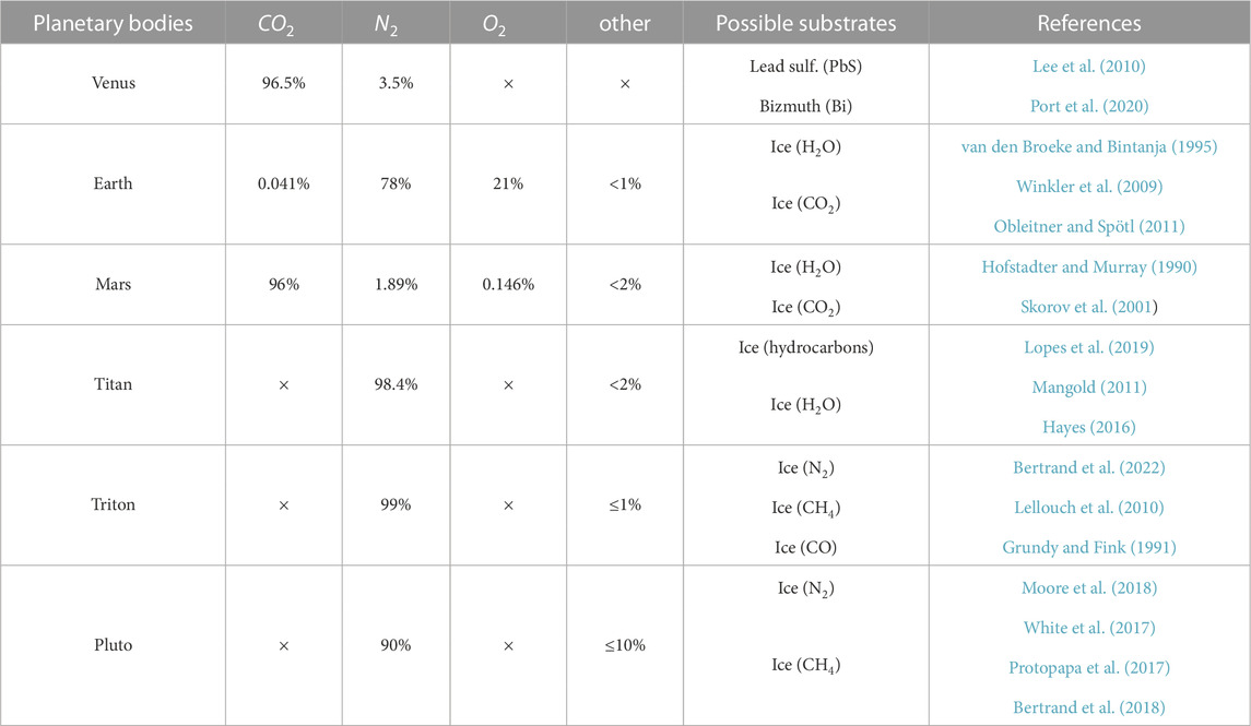
TABLE 1. Main composition of the atmospheres of various planetary bodies likely to undergo sublimation/deposition on their surface.
2.3 Planetary examples of sublimation waves
Sublimation waves have been identified as markers of net sublimation by Bordiec et al. (2020) because their morphological and kinematics characteristics (wavelength, migration velocity, erosion rate, formation time) can be linked to their environmental conditions of formation (wind velocity, viscosity, pressure, temperature, diffusion coefficient). On Earth, transverse linear bedforms produced by sublimation are rare. Comprehensive data collected for two terrestrial natural examples and for an original sublimation experiment of CO2 are synthesized in this section. They are completed by new observations on Mars and Pluto, that have vast icy expanses with distinctive linear dune-like patterns. All the data are summarized in Table 2 (white boxes). In all these environments, linear and transverse bedforms appear. However, they are quite different in scales and involve different compositions of the icy substrate and the atmosphere (Table 1). Despite those differences, the winds that flow on these surfaces are always turbulent and of many decades great in height in comparison to the wavelength.
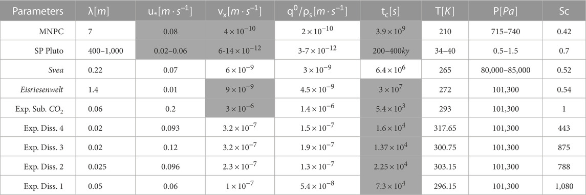
TABLE 2. Average values of the parameters involved in the three scaling laws of the transverse linear bedforms, for each environment where abalation waves have been observed: the upper part of the table concerns planetary environments (Forget et al., 2017; Millour et al., 2018; Bertrand et al., 2020; Bordiec et al., 2020), the lower part, the terrestrial and experimental analogues in sublimation (Bintanja, 1999; Obleitner and Spötl, 2011; Bordiec et al., 2020) and the third part the analogous experiments in dissolution (Blumberg and Curl, 1974). The values correspond either to measurements (white cells) or to predictions from the laws (grey cells). λ = wavelength, u* = friction velocity, vx migration velocity, q0/ρs = erosion rate, tc = characteristic time, T = temperature, P = pressure, Sc = Schmidt number.
2.3.1 Sublimation waves on water-ice - Earth
The first natural terrestrial example is located at Svea station, Antarctica (Figure 2A), on the Blue Ice Areas (BIAs), which are smooth and compact icy surfaces. The atmospheric pressure and ambient temperature conditions are in the range of 800 hPa and 850 hPa and 265 K during the austral summer, respectively (Bintanja, 1999). Mass transfer is induced by sublimation at a rate of q0/ρs ∼ 10 cm ⋅yr−1 estimated in the absence of wind (Bintanja et al., 2001). With such a sublimation rate, the growth time of the sublimation ripples is about
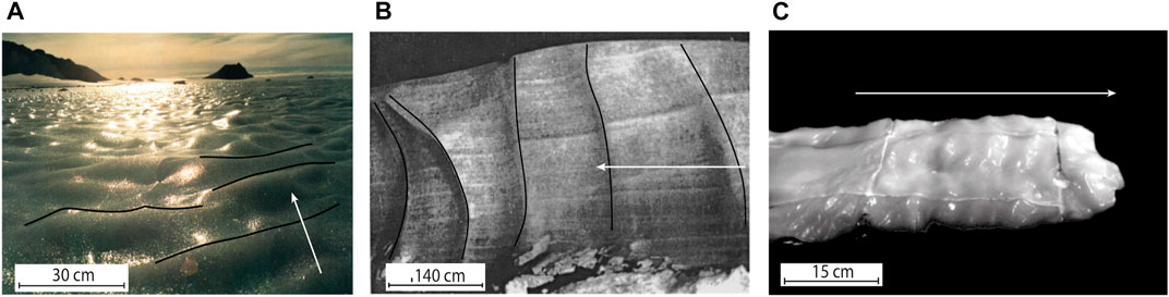
FIGURE 2. Sublimation waves: (A) on Blue Ice areas (Bintanja et al., 2001); (B) on the wall of the Eisriesenwelt ice cave (Obleitner and Spötl, 2011); (C) on CO2 ice in an atmospheric wind tunnel (Bordiec et al., 2020). White arrow indicates the wind direction adapted from (Bordiec et al. 2020).
The second example is the Eisriesenwelt ice cave, Salsbourg, Austria (Figure 2B), where dry, cold air (T = 272 K) from outside (p = 1 atm) also flows in turbulently and causes the walls to sublimate in winter. The dimensions of the sublimation waves of 1.4 m are much larger than those observed in Antarctica while the wind speed of the order of ≃ 0.2 m ⋅s−1 is 10 times lower, so the friction velocity is smaller with u* ≃ 0.01 m ⋅s−1 (Obleitner and Spötl, 2011). Although mentioned, migration has never been measured and the emergence of the waves takes less than 1 year, before ice melts in summer (Curl, 1966), with a sublimation rate q0/ρs ∼ 1.42 cm ⋅yr−1.
2.3.2 Sublimation waves on CO2 ice - Wind tunnel experiment
An analogical experiment to sublimation waves of water ice in Antarctica was proposed by Bordiec et al. (2020) to test whether the coupled action of wind and sublimation can generate bedforms in a windy controlled environment, in the atmospheric wind tunnel in Nantes, France (LHEEA, UMR6598), using CO2 ice as it sublimates at ambient pressure and temperature conditions (p = 1 atm, T = 293 K). In net ablation with a sublimation rate measured in the absence of wind of 1.4 × 10⁻⁶ m ⋅s−1, these ice blocks subjected to a turbulent flow at U = 6 m ⋅s−1 with u* ≃ 0.2 m ⋅s−1 presented, after ∼ 4 h, centimeter-scale undulations on their surface about 6 cm in wavelength (Figure 2C). Migration of the ripples could not unfortunately be measured but predicted to be of the order of 1. cm ⋅h−1 by Bordiec et al. (2020).
2.3.3 Sublimation waves on water-ice - Martian North Polar Cap
To explore the possibility that these type of new morphological markers exists among sublimation patterns described on the MNPC, images of the region located at the boundary between Boreales Scopuli and Olympia Cavi (82°N, 120°E) were studied by Bordiec et al. (2020), when water ice is exposed to sublimation for a period between Ls = 90° and Ls = 135°, with a maximum between Ls = 100° and Ls = 120° (Pankine et al., 2010). During this period, surface temperature is (T ≃ 210 K) and vapour pressure (P ≃ 730 Pa) (Pankine et al., 2010) with a sublimation rate estimated at q0/ρs ∼ 2. × 10–10 m ⋅s−1 (Chittenden et al., 2008). These patterns are identified in Figure 3, they are linear and parallel ridges, generally oriented along the North-South direction. Nguyen et al. (2020) suggested that these shapes are different from classical Martian aeolian dunes and Bordiec et al. (2020) propose that the process responsible for their formation is sublimation coupled with a turbulent winds. The turbulent boundary layer thickness about ≃ 10 km (Pankine and Tamppari, 2015) is greater than the observed wavelength with λ ≃ 7 m. The katabatic winds flow in summer (Howard, 2000; Kauhanen et al., 2008; Petrosyan et al., 2011) over the region. We can estimated the wind speed around ≃ 2.5 m ⋅s−1 (u* ≃ 0.08 m ⋅s−1) using GCM data base (Forget et al., 1999; Millour et al., 2018) at 100 m above the surface of this region. The orientation of the prevailing winds in this region, deduced from mesoscale numerical simulations of Smith and Spiga (2018), is east-west. This is confirmed by the orientation of the wind streaks around a crater located in the same region (Bordiec et al., 2020). The bedforms are therefore transverse, perpendicular to the prevailing winds.
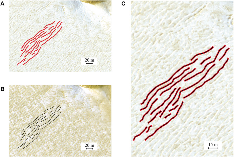
FIGURE 3. Comparison of the location of the crests of the sublimation waves of the MNPC between 2008 and 2009 during the northern Martian summer (Ls =115°). (A) Image ID HiRISE: PSP_009689_2645; credit: NASA/JPL/University of Arizona obtained on 20 August 2008. Spatial resolution is 25 cm/pixel. Crests are highlighted in thick red lines. (B) Image ID HiRISE: ESP_062580_2645; credit: NASA/JPL/University of Arizona obtained on 2 December 2019. Spatial resolution is 25 cm/pixel. Crests are highlighted in thin black lines. (C) Zoom of the surface (PSP_009689_2645, 2008) with superimposed crest lines from figures (A, B). The undulations are considered as close as possible to the crater, which serves as a fixed reference for georeferencing the images. The superimposed crest lines indicate that they have not moved between 2008 and 2019, or by so little that this difference could not be detected.
To complete the morphological analysis with a kinetic study of these objects, we compare all the HiRISE images at the horizontal resolution of 25 cm/pixel, available in the region since the camera was operational in 2008. Ripple crests over this region have been located between 2008 (Figure 3A) and 2019 (Figure 3B) during the northern Martian summer (Ls = 115°). The selected crests are considered to be as close as possible to the crater that serves as a fixed reference for georeferencing the images. Figure 3C shows that the crest lines overlap and does not allow the observation of any evolution in time of these undulations between 2008 and 2019, or by such a small amount that this difference could not be detected.
2.3.4 Candidate sublimation waves on CH4 ice – Sputnik Planitia, Pluto
At present, the mean surface temperature of Pluto is around T = 37 K and an atmospheric pressure between p = 0.5 and 1.5 atm. Pluto shares similarities with Mars: a tenuous atmosphere with a complex climatic system driven by the redistribution cycles of volatile ices. Pluto’s atmosphere is very rich in N2 and the conditions at its surface are such that it is now known that the successive cycles of sublimation and condensation of N2 but also CH4 are not only active processes but also partly responsible for the diversity of landscapes (Figure 4) on the surface (Bertrand et al., 2018; Bertrand et al., 2019). Among the great diversity of landforms on Pluto, Sputnik Planitia (Figure 4A), a large basin covering more than 30° in latitude composed of a complex mixture of N2 ice, and to a lesser extent CO and CH4 ices (Schmitt et al., 2017), is the most emblematic. Sublimation is currently dominant above 15°N, at a rate estimated to q0/ρs ∼ 3 − 7 × 10⁻¹² m ⋅s−1, while condensation dominates below (Bertrand et al., 2018). This plain contains many characteristic shapes (Figure 4B), such as polygonal cells over ≃ 10 km wide interpreted as resulting from thermal convection of the ice (McKinnon et al., 2016; Trowbridge et al., 2016; Morison et al., 2021) and bordered by pits over 100 m deep. These remarkable shapes provide an additional argument to that of the absence of craters on the whole Sputnik Planitia, in favor of the hypothesis of a geologically young and active surface
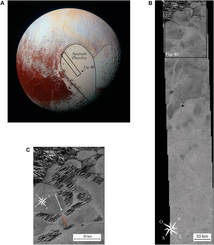
FIGURE 4. Pluto and its regions of interest, 14 July 2015 (credit: NASA/JHUAPL/SwRI). (A) Global view of Pluto in colour, taken by the Ralph/Multispectral Visual Imaging Camera (MVIC) on New Horizons. The “heart” of Pluto is dashed and the region of Sputnik Planitia is highlighted. (B) Image of part of Sputnik Planitia, taken by the Long Range Reconnaissance Imager (LORRI), at a resolution of 77 to 85 m/pixel. (C) Zoom on the linear and regularly spaced crests of the western region of Sputnik Planitia bordered by the al-Idrissi mountains and superimposed on polygonal cells. The crest lines are underlined in black while the white arrow indicates the wind direction deduced from the streaks (in orange) and the surrounding topography (modified from Telfer et al. (2018)).
A surface texture consisting of pits, typical of the circular shapes created by sublimation and regularly distributed in space, is the dominant texture in the southern part of the plain (Moore et al., 2017). To the northwest, the basin is bounded by the al-Idrissi mountains composed of water ice, next to which, over an area of ≃ 75 km from these mountains (latitude ≃ 30°N, longitude ≃ 160°E, Figure 4C), linear ridges regularly spaced (0.4–1 km) were observed by Telfer et al. (2018) on a substrate composed of CH4 and N2. With distance from the mountains, these ridges become spaced further apart and are arranged in patches. Wind streaks behind certain obstacles also attest to the direction of the wind, consistent with the local topography, and that seems to be perpendicular to the orientation of these ridges (Telfer et al., 2018). Indeed, the winds on Sputnik Planitia seem to be locally induced by the condensation and sublimation of N2 (Forget et al., 2017) and by the so-called katabatic gravity flow on topographic slopes that are linked to the temperature difference between the colder surface and the warmer atmosphere. Winds are generally turbulent near the surface (boundary layer of thickness ≃ 15 km) and modeling of their circulation indicates that their speed could reach several meters per second (at 20 m above the surface) although it would generally be less than 1 m per second (Forget et al., 2017). Since the strongest winds are expected to occur where the topographic gradients are greatest the northwestern part of Sputnik Planitia on which the ridges appear would correspond to a very windy region (Telfer et al., 2018) and areas with more widely spaced ridges to more moderate winds.
One of the interpretations proposed so far to explain the formation of the linear ridges in northwestern of Sputnik Planitia is that they are dunes formed by grains of CH4 ice, whose movement would be initiated by sublimation because the friction velocity of the local winds is not strong enough to reach the threshold friction velocity to set the grains in motion, and would then be maintained by local winds (Telfer et al., 2018). Nevertheless, Gunn and Jerolmack (2022) show that even the threshold to maintain grain transport (friction velocity is about u* = 1. m ⋅s−1) is too high for the proposed wind speeds over Sputnik Planitia. By analogy with observations of sublimation ripples in Antarctica, in ice caves and on the MNPC, it would seem that the main ingredients required in each of these environments are also present on Sputnik Planitia, suggesting that an alternative hypothesis could be that these ridges are the result of sublimation (without grain transport) coupled with turbulent winds.
3 Dissolution waves on soluble rocks
Ablation waves occur on solid substrates that are subject to mass transfer at their surface. The flow of liquid like water can dissolve some rocks. If dissolution waves, i.e., flutes/solution ripples are mentioned and visibly widespread (Ford and Williams, 1989; Ginés et al., 2009), complete natural data sets on the subject are paradoxically lacking. The description of their form, occurrence and the environments in which they develop, through natural examples and laboratory experiments, borrowed from a field analysis and the existing literature is the subject of this section. The only complete experiment on the specific subject of flutes/solution ripples on a dissolving solid substrate of which average parameters measured are given in Table 2 (white boxes), is the dissolution laboratory experiments run by Blumberg and Curl (1974).
3.1 Soluble rocks on Earth
Carbonate rock and evaporite outcrops are widespread on Earth and very often form complex systems of landscapes dotted with caves and underground networks in which water circulates. The type of system that is created on these soluble rocks are called karsts. Karst landforms occupy no less than
3.2 Development of dissolution waves
3.2.1 Mineral composition
Soluble rocks and particularly carbonate rocks are composed of minerals such as calcite and dolomite, and evaporitic rocks are composed of sulphates or chlorides. Evaporite karsts are mainly composed of gypsum (CaSO4, H2O), the most common sulphate mineral among evaporites. After carbonates, it is indeed the mineral that precipitates the fastest, before its dehydrated forms (anhydrite CaSO4 and halite NaCl). Since it only appears after gypsum and because the waters of lagoons and intertidal zones are generally renewed before it precipitates, halite is less widespread, except in the case of arid regions where the waters are endoreic, i.e. hydrologically closed lakes that do not drain to the sea. Salt karsts are therefore limited to patches in these deserts and, despite the fact that they are ephemeral and relatively young (for those that currently exist) in view of the high solubility of halite and its fragility, remain little studied (Frumkin, 1994; Frumkin, 2013).
3.2.2 Kinetics of dissolution
The process of accumulation and removal of water-soluble rocks is chemical: dissolution/precipitation reactions are mainly involved. When a rock dissolves in water, some or all of its individual minerals disintegrate into individual ions or molecules that are then diffused into the solution. Calcite, gypsum and halite dissolve by dissociation according to the reactions given in Table 3. They dissolve in water, the viscosity of which depends mainly on the temperature (Kaufmann et al., 2014).
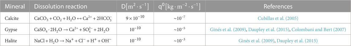
TABLE 3. Dissolution reactions, orders of magnitude of diffusion coefficients D and dissolution fluxes q0 of the main minerals constituting soluble rocks, at 25°C and 5< pH <9, from Ford and Williams (1989); Morse and Arvidson (2002); Daupley et al. (2015).
Classically in chemical kinetics, the dissolution of a solid in a solution is separated into several distinct physical or chemical steps (Morse and Arvidson, 2002): (i) the transport of the reactive agents from the liquid to the solid surface, (ii) the adsorption of reactive substances on the surface, (iii) the chemical reaction between the adsorbed reagents and the solid surface, which may also contain several steps, (iv) the desorption of products into solution, (v) the transport of products and their diffusion in the solution.
The overall kinetics of the transfer is therefore limited by which of these steps is the slowest. For calcite, which has more dissolution-precipitation reactions than gypsum or halite, the kinetics is influenced by numerous parameters, such as the acidity (pH) the partial pressure of CO2
The kinetics of dissolution is thus controlled sometimes by transport, sometimes by chemical reaction, and sometimes both at the same time, that leads to a mixed behaviour. Thereafter, we are interested in processes dominated by the transport of particles (vapour, ions in solution) by advection-diffusion in a flow. In this case, the dissolution rate defined by q0/ρs is very small compared to the friction velocity u* of the flow (Table 2).
3.3 Terrestrial examples of dissolution waves
3.3.1 Dissolution waves on limestone - Saint-Marcel d’Ardèche cave, France
The linear transverse undulations produced by dissolution exist mainly on the walls of caves in soluble rocks, as in the cave of Saint-Marcel d’Ardèche, France, in calcite. It is characterised by large volumes, a rich concretion and shows many forms of dissolution on its walls. The galleries of the network contain a fine detrital filling composed of beige and red mica sands and clays. Between the demarcations linked to the successive sections of the gallery, transverse and linear ridges have developed, among other forms (Figure 5).
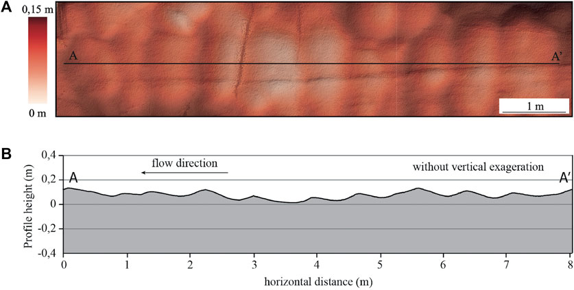
FIGURE 5. Typical shape of the dissolution waves visible on the wavy walls of the Galerie des Peintres of the Cave in St-Marcel d’Ardèche, France. (A) Raster image of the wall, obtained by interpolation of LIDAR point clouds. The black line symbolises the cross-sectional AA’ line that allows the typical profile to be visualised. (B) Typical profile according to section AA’.
In order to characterize these forms morphologically, a few selected walls on network I were scanned using a portable LIDAR, in the Gallerie des peintres or Gallerie des maçons. The topographic data acquired with the LIDAR allowed the production of 3D surfaces by interpolation of point clouds (Figure 5A) and 2D profiles of the shapes (Figure 5B). The general shape of the ripples is not sinusoidal but some periodicity of the peaks is observed. With a wavelength ≃ 1 m and an amplitude ≃ 0.1 m, their aspect ratio is of the order of Ra ≃ 0.1. Their transverse profile is asymmetrical and has a steeper slope on the downstream side than on the upstream side. No information on the formation of these undulations can be acquired so controlled experiments are required to complement Table 2.
3.3.2 Dissolution waves on gypsum - Laboratory experiments
The experiment of Blumberg and Curl (1974) consists in reproducing dissolution waves on a soluble substrate in the laboratory (Figure 6). They study their stability, through the wavelength, the migration, the general temporal evolution, the dissolution rate and more generally, the mass transfer that takes place. Their choice of substrate is gypsum (calcium sulphate hemihydrate), whose dissolution is ensured throughout the experiment by maintaining a reagent concentration at 10% from saturation, by replacing part of the solution with the same volume of fresh water continuously. The experiment is carried out in a hydrodynamic tunnel of cross-section 15.25 cm × 15.25 cm, imposing a hydrodynamic boundary layer of ≃ 7.6 cm. The temperature is continuously monitored and the flow velocity U is measured at all times by pitot tubes. The block of gypsium, of size 76.2 cm × 15.25 cm × 12.7 cm, is placed in the centre of the tunnel.
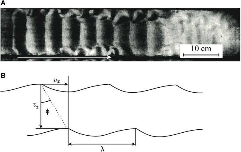
FIGURE 6. Dissolution experiment adapted from Blumberg and Curl (1974). (A) Dissolution waves (Exp. 1). The wavelength is 5 cm. The white arrow indicates the direction of flow. (B) Profile and geometrical parametrisation of the dissolution waves. The lower profile corresponds to its evolution over time, after dissolution. ϕ is the propagation angle, and vx the migration velocity.
The authors indicate that the length of the hydrodynamic tunnel is not sufficient to create dissolution waves spontaneously, so grooves transverse to the flow were made on the surface of the block at regular intervals, on which the ripples are supposed to develop. The authors admit that this approach does not allow the exact determination of the equilibrium situation of the dissolution waves, i.e. the growth time at which they should have emerged spontaneously from an initially flat surface. The disturbance of the topography predefined by these grooves seems however not to influence the wavelength and the final profile of the dissolution waves since the various tests carried out by Blumberg and Curl (1974) with several extreme intervals, demonstrate that the ripples develop on the grooves and then evolve by gradually increasing or decreasing the wavelength progressively until a certain common equilibrium is reached.
Due to combined effects of dissolution and different turbulent flow velocities, these dissolution waves have a centimeter spacing (2–5 cm and a millimeter amplitude and migrate at different velocity 1–3.2 × 10⁻⁷ m ⋅s−1 in the direction of flow. During their series of experiments, the device allowed the measurement of the parameters ϕ, the propagation angle and vz, as well as the local values of the slopes θ, that allowed them to generalize the shape of the profiles obtained (Figure 6A). Their measurements (see Blumberg and Curl (1974) for details of the methods) provide an estimate of the local vertical dissolution rate vz = q0/ρs, where q0 is the flux density at the wall. Using the measured values of the propagation angle ϕ in the Blumberg and Curl (1974)’s experiments, the horizontal migration velocity can be deduced geometrically (see Figure 6B) as a function of the propagation angle and the sublimation rate:
The main results of these experiments are listed in Table 2 (white cells). It should be noted that the growth times of bedform formation have not been measured but could be estimated. Indeed, all the data collected in Table 2 are complemented by additional calculations (grey cell) from the scaling laws presented in next section 4.
4 Scaling laws for ablation waves: a unified model
Ablation waves involve solid substrates, such as ice (§2), but are also found on soluble rocks (§3). Perturbations of a flat substrate, without characteristic or periodic length, disturb the flow that modifies the mass transfer that in turn modifies the topography. This positive feedback can initiate an unstable system, i.e. one that does not return to its initial state following a disturbance or disturbances. The role of morphogenesis is to consider how to relate the characteristics of topography to those of flow and mass transfer. While several approaches exist, instability theory and in particular linear stability analysis, which relates the growth of disturbances to the growth of instabilities, seems to be the most relevant (Gallaire and Brun, 2017).
4.1 Ablation by sublimation or dissolution: an analogous instability mechanism
Mass transfers shape solid substrates by ablation under a turbulent flow. Sublimation is a physical transformation of phase change between the solid and vapour phase without passing through the liquid phase, whereas dissolution is based on chemical reactions between ions in solution and molecules. These transfers are therefore different in nature but both involve a variation in enthalpy and have a similar formulation of their equilibrium (saturation vapour pressure and equilibrium constant, resp.). The direction of the transfer is in both cases conditioned by the value of a relative quantity that determines whether the system is saturated or not (relative humidity and saturation index, resp.). The kinetics of the transfers can be considered at the microscopic scale (kinetic theory, chemical kinetics, resp.) at the interface or extrapolated to the continuous medium when the transport of particles (vapour, ions in solution, resp.) is based on advection-diffusion in a flow. In both cases, the quantification of the material flow is proportional to the difference between the concentration and the equilibrium concentration, weighted by a kinetic coefficient depending on the type of transfer. This approximation is valid at the macroscopic scale where the transport of vapour or ions in solution, resp., is by advection and diffusion in a turbulent near-wall flow.
The sublimation and dissolution waves could be analogous as long as the instability mechanism responsible for their development is robust (Gallaire and Brun, 2017). If so, their shape and their kinetics depend on a combination of physical parameters, through dimensionless numbers driving the problem, with at least one of these numbers being conserved whatever the type of transfer so that there is similarity. The friction velocity u* and the viscosity ν of the underlying turbulent flow seem to control the characteristic length scale λ of the waves through a coefficient whose value seems to be linked to the type of transfer that is characterized by the ratio between the viscosity of the flow ν and the diffusivity coefficient D of the substrate in the flow. As can be seen in Table 2 (i) the Schmidt number ν/D depends on the type of transfer, from
4.2 Stability analysis of the coupled ablative mass transfer and near-wall turbulent flow
The objective of the temporal stability analysis is to study the stability of the solid-substrate/flow interface with time. The interface profile is generally written:
where ζ0 is the amplitude,
The ablation wave emerge if σ > 0 (they are unstable), while they disappear if σ < 0 (they are stable). Their migration speed that is equal to −ω/k is in the direction of flow if ω < 0 and in the opposite direction of flow if ω > 0. The determination of the dispersion relation of the system makes it possible to highlight the values of k for which σ > 0 and to identify the most unstable mode for which σ is maximal.
The linear approach works even if the aspect ratio
By studying the stability of the coupled flow dynamics and mass transfer system, it has been shown that the combined effect of winds and sublimation (Bordiec et al., 2020) or water flow and dissolution (Claudin et al., 2017) lead to the formation of ablation waves, i.e. σ > 0, for a given wavelengths range in a transition regime between laminar and turbulent flow for a wall-Reynolds number based on the bedform’s wavelength
4.2.1 Dimensionless numbers of the problem
Afterwards, the following configuration is considered: a flow of many decades great in height with respect to the wavelength of the bedforms, in a hydrodynamically smooth regime (Rr → 0), by limiting to the linear effects of the instability. From the parameters and dimensional considerations, it is possible to highlight four dimensionless numbers characteristic of the problem.
(i) The Schmidt number Sc compares the effects of momentum and mass diffusivity. It is defined by
(ii) The dimensionless wavenumber is the one that controls the near wall regime:
(iii) The dimensionless growth time is defined by:
(iv) The dimensionless number pulsation ω+ is defined by:
The ratio −ω+/k+ = tan(ϕ) defines the propagation angle.
4.2.2 Dependance on the Schmidt number
Since the diffusion coefficient is much lower in liquids than in gases, the order of magnitude of Sc is typically 103 in liquids, while it is only unity in gases (Incropera et al., 2007). Although different, the values of the Schmidt number in the different environments described § 2 for sublimation remain of the same order of magnitude (Sc ≃ 1) whereas for dissolution, the experiments described in § 3, the Schmidt number is variable, between 102 and 103 (Table 2). The dispersion relation displayed in Figure 7 explores the instability. In the (Sc, kν/u*) plane, the unstable domain is defined on Figure 7A by a shaded area corresponding to σ+ > 0 for which the scaled wavenumbers k+ belongs to the near-wall regime of laminar-turbulent transition. The maximum growth rate
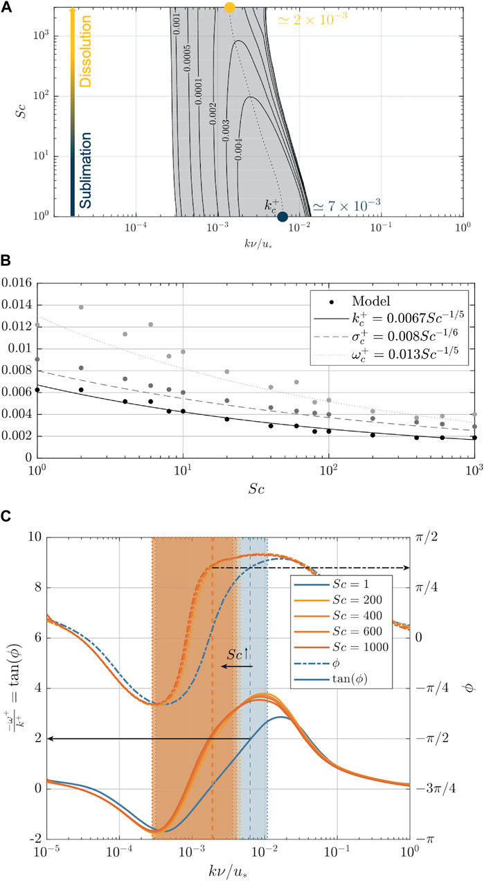
FIGURE 7. Influence of the Schmidt number on the dimensionless parameters of the dispersion relation. (A) Stability diagram in the (Sc; kv/u*) plane. The shaded area corresponds to the unstable domain (σ+ > 0) and the values displayed are those of the σ+ isocontours. The dashed line represents the most unstable mode
Figure 7B shows the evolution of the dimensionless numbers of the dispersion relation, characteristic of the instability, as a function of the increasing Schmidt number. The numerical results show that
The experimental propagation angle ϕ, defined in Section 3.3.2 (Figure 6B), appears to be relatively constant (ϕ ≃ 63.5°) in the dissolution experiments (Blumberg and Curl, 1974) for different Schmidt numbers. This can be explained by the fact that
4.3 Validation and prediction
Scaling laws have been developed in sublimation by Bordiec et al. (2020) to relate the morphological and kinematic characteristics of sublimation waves to the characteristics of the environment in which they occur. Since the type of transfer does not affect the instability, the laws can be generalized and are valid for both sublimation and dissolution. However, previously (§4.2.2) shows that the characteristic numbers of the most unstable mode
4.3.1 Wavelength
The first scaling law relates the wavelength λ to the viscous length
where
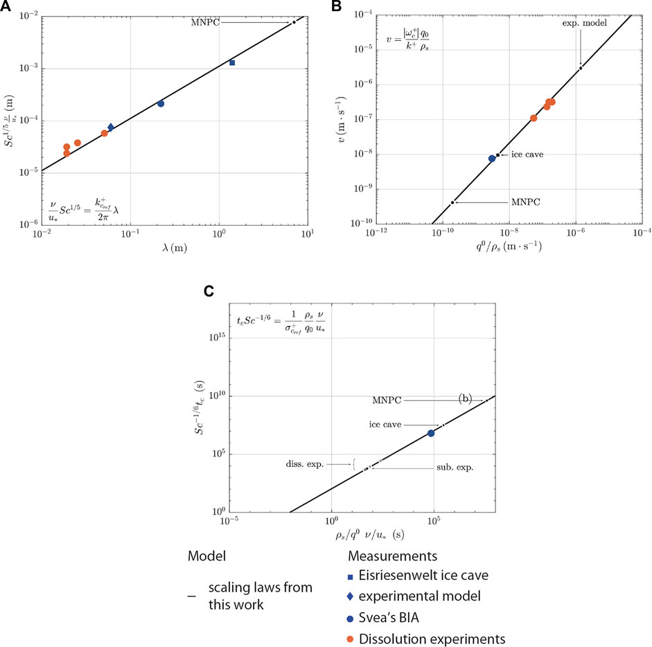
FIGURE 8. Scaling laws (black lines) for the unified model of sublimation waves on Earth (blue symbols: square = ice cave; circle = BIAs; diamond = CO2 experiment) and dissolution waves (orange symbols). Symbols represent measured quantities, black dots are predictions. (A) First theoretical scaling law relating the wavelength λ to the viscous length v/u* (solid line), derived from the dispersion relation and superimposed on the measurements on sublimation waves (in blue) and on dissolution waves (in orange). The dependance on the Schmidt number is included to present an unified model. (B) Second theoretical scaling law relating the migration velocity v to the ablation rate q0/ρs (solid line), derived from the dispersion relation and superimposed on the measurements (symbols) on the natural and experimental systems (orange for the dissolution experiment (Blumberg and Curl, 1974); blue for the BIAs (Bintanja et al., 2001)). The positions of the sublimation waves observed on the surface of the MNPC, in the ice cave of Eisriesenwelt and in the experimental model (v unknown because never measured) are indicated by black dots superimposed on the scaling law. The non-dependance on the Schmidt number shows the analogous character of dissolution waves as a terrestrial analogue of the sublimation waves. (C) Third theoretical scaling law relating the growth time t to the ablation rate q0/ρs and the viscous length v/u* (solid line), derived from the dispersion relation and superimposed on the measurements on the unique measure natural system (on the BIAs (Bintanja et al., 2001)). The positions of the sublimation waves observed on the surface of the MNPC, in the ice cave of Eisriesenwelt, in the experimental model are indicated by black dots superimposed on the scaling law and for the dissolution experiment (Blumberg and Curl, 1974) are indicated by black circles superimposed on the scaling law. The dependance on the Schmidt number is included to present an unified model.
This law shows that the wavelength λ is inversely proportional to the friction velocity u* for a given flow whatever the substrate: the faster the velocity, the smaller the wavelength. This is in accordance of what has been observed for sublimation waves on BIA’s (Weller, 1969; Mellor and Swithinbank, 1989; Bintanja et al., 2001). For higher viscosity, depending on the pressure of the atmosphere as for instance Pluto’s kinematic viscosity that is 40 times higher than martian’s viscosity because of the lower pressure of the atmosphere, larger wavelength have to be found for comparable friction velocity at equivalent Schmidt number
4.3.2 Migration velocity
The second scaling law proposed by Bordiec et al. (2020) related to the migration velocity of the ablation waves is proportional to the average value of the ablation rate
where
Because this law shows that the migration speed of these ablation waves depends only on the ablation rate (Figure 8B), the law can be used to predict the migration rate or, conversely, to estimate an ablation rate if the migration velocity is measured. For example, the predictions for the sublimation waves observed on the surface of the North Polar Cap of Mars, in the ice cave of Eisriesenwelt and in the experimental CO2 model (Table 2, grey cells) are indicated by black dots superimposed on the scaling law. The predictions made where the migration velocity has not been measured are realistic for the ice cave and the CO2 sublimation experiment but remain to be confirmed with further experiments or in situ campaign. Using the measured values of the propagation angle ϕ in the Blumberg and Curl (1974)’s experiments 1-4 (ϕ = 62°; 60°; 59°; 64°, resp.), the migration velocities have been deduced geometrically (see Figure 6B) in Table 2, white cells. They are in perfect agreement with the predictions of the law for experiments 1-4 (1.1 × 10⁻⁷, 2.6 × 10⁻⁷, 3.4 × 10⁻⁷, 3.3 × 10⁻⁷, resp.).
4.3.3 Growth time
The third law relates the characteristic growth time to the viscous length and the ablation rate, and is therefore dependent on the flow and type of transfer (Figure 8C):
where
5 Charts for estimating friction velocity in different environments
The scaling laws presented in the previous section §4 have been developed to propose a unified model of ablation waves for dissolution and sublimation. To create a tool for the direct application of the laws in environments as diverse as ice caves, icy surfaces, laboratory experiments, planetary surfaces, karsts and limestone, gypsum and halite surfaces, we present these results in the form of specific charts. Since the coefficients kc +, ωc + and σc + of the laws differ in dissolution and in sublimation, we design a graphical representation of family of curves for each type of transfer: Figures 9, 10 for sublimation, depending on the composition of the atmosphere (Table 1); Figure 12 for dissolution.
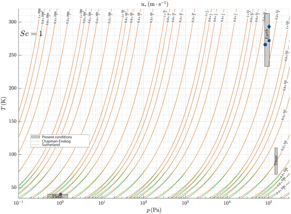
FIGURE 9. Graphical representation of the first law for sublimation in a N2 rich atmosphere (Sc = 1). Knowing the wavelength of the sublimation waves, one can determine the friction velocity locating the ambient pressure and temperature over the wave field on the planetary body considered. The grey rectangles correspond to the pressure and temperature ranges for Earth, Titan and Pluto. The blue symbols correspond to the natural examples of sublimation ripples studied (square = ice cave; circle = BIAs; diamond = CO2 experiment). The purple symbol is for Pluto.
Considering that the basic quantities measured and/or measurable in the application environments consist mainly of ambient pressure and temperature (Table 2), the calculations to obtain the family of curves have to be adapted to these two parameters. For exemple in Figure 12, by plotting the temperature of water at ambient pressure, it is possible to estimate u* thanks to the first scaling law (Eq. 6) if a measure of λ of dissolution waves exists and vice versa. This presupposes an implicit calculation of the viscosity following different viscosity laws (e.g. Sutherland and Chapman-Enskog, Chapman et al. (1990)). In most cases, the choice of the viscosity law does not affect these estimates because the Sutherland and Chapman-Enskog laws are superimposed for the mean pressure and temperature ranges concerned in most of the relevant planetary environments (Figure 1, grey boxes, p > 10–2 Pa). In sublimation, and by using the first law, the friction velocity can be represented as a function of pressure, temperature and observed wavelength, for all N2-rich atmospheres in Figure 9. This allows application to the Earth, Titan or Pluto. CO2-rich atmospheres in Figure 10 allow applications to Venus and Mars.
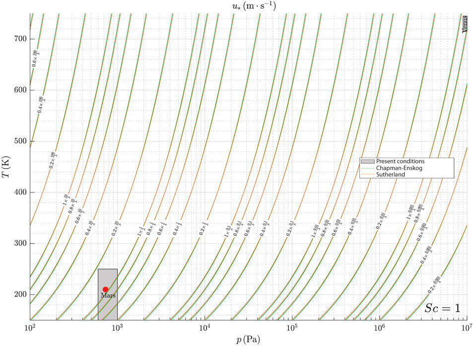
FIGURE 10. Graphical representation of the first law for sublimation in a CO2 rich atmosphere (Sc = 1). Knowing the wavelength of the sublimation waves, one can determine the friction velocity locating the ambient pressure and temperature over the wave field on the planetary body considered. The grey rectangles correspond to the pressure and temperature ranges for Mars and Venus. The red circle represents the environmental condition over the sublimation waves that have been identified on the MNPC.
The other two laws (Eq. 7, 8) are more difficult to represent graphically as a function of pressure and temperature alone. Indeed, these laws imply the ablation rate that can only be constrained on the condition of knowing the temperature T, the pressure p but also the temperature at the interface Tint and a value of relative or specific humidity in the case of sublimation, and the temperature, the solubility, the concentration and the pH in the case of dissolution. To simplify the representation of these laws, they can be combined to give:
with
5.1 Application to sublimation waves
In icy planetary environments potentially subject to sublimation (§2.2, Table 1), the main gases involved are nitrogen N2 and carbon dioxide CO2. Two charts are proposed for atmospheres rich in N2 (Figure 9) and CO2 (Figure 10). The viscosity of these gases as a function of temperature is relatively well known at standard pressures. This is why a first tool to deduce u* and/or λ is proposed from the knowledge of temperature and pressure. The possible ranges of variation in p and T in the current configuration of each planetary environment are represented by grey areas on Figures 9, 10. Except for Pluto, where pressure changes induce strong viscosity variations, the number of curves crossing the environments is generally small, that induces reduced possibilities of u* − λ combinations at given pressure and temperature.
The natural examples (BIAs, ice cave) and laboratory experiments of CO2 ice presented in §2.3.1 and §2.3.2 are plotted on Figure 9 (see blue symbols) for N2-rich atmospheres. It makes thus possible to find an estimate of u* or λ. For the sublimation waves observed on the MNPC in §2.3.3 (red symbol in Figure 10), knowing the average atmospheric pressure and the temperature near the surface (Table 2) where they have been observed, one can obtain the friction velocity, simply by replacing λ by its value. The value extracted from the corresponding curve is
In Figure 9, the current conditions of Pluto have been indicated by a purple circle in the grey area. The same application as above to the observed wavelength of Sputnik Planitia in §2.3.4 gives
The combination of scaling laws allows the ablation and the migration rates to be plotted on the same graph, independently of the nature of the substrate and the flow. Reading Figure 11 then allows to know the growth time tc from the knowledge of the ablation rate and the wavelength or from the migration velocity and the wavelength. This is relevant for the surfaces of BIAs and on the North Polar Cap of Mars. For the special case of ice caves, where the estimation of the sublimation rate is more difficult, it can be obtained by knowing the growth time and the wavelength.
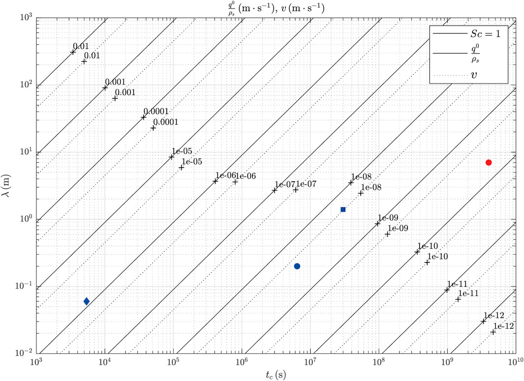
FIGURE 11. Combination of the second and third laws for sublimation (Sc =1). Locating the wavelength on the y-axis and drawing a line upward to the curve representing the sublimation rate or the migration velocity, the formation time can be determined by reading thanks to a line drawn vertically. The blue symbols represent the natural examples of sublimation ripples studied (square = ice cave; circle = BIAs; diamond = CO2 experiment) and the red circle represents the sublimation waves identified on the MNPC.
The different validated applications are shown on Figure 11 (see blue and red symbols). As the data collected are isolated points in their parameter scale, given that the environmental conditions and sometimes even the type of icy substrate are different, there is no systematic measurements of bedform’s wavelength change when continuously varying some control parameter. In order to investigate a range of wind velocity and fluid viscosity in a controlled environment, this chart will be helpful tool for scaling laboratory experiments of sublimation. Such experiments would make it possible to characterize these sublimation waves in terms of their growth time, ablation rate and migration velocity.
5.2 Application to dissolution waves
The dissolution rates of limestone, gypsum and halite are widely studied and constrained in various situations (Table 3). The dissolution takes place in water whose viscosity depends mainly on temperature (Kaufmann et al., 2014). Since the temperatures concerned by this type of reaction are temperatures for which the kinematic viscosity of pure water is well known, the viscosity is injected directly into the law. Despite the lack of existing data, Blumberg and Curl (1974)’s experiments (§3.3.2) allow the abacus chart to be validated by entering the values of Table 2 in the form of red symbols in Figure 12A. Choosing this type of graphical representation constitutes a tool for finding the friction velocity u* and the velocity of the flow by extrapolation (Bordiec et al., 2020), as a function of the temperature on the one side and the measurement of a wavelength on the other side. A quick application to the transverse linear undulations observed in the Cave of St-Marcel d’Ardèche (§3.3.1) assuming that Sc = 1,000 and that the temperature is of the order of T = 10°C, the friction velocity u* from figure Figure 12 is ≃ 0.06 m ⋅s−1, which leads to a very low flow velocity at z = 1 m of the wall of the order of
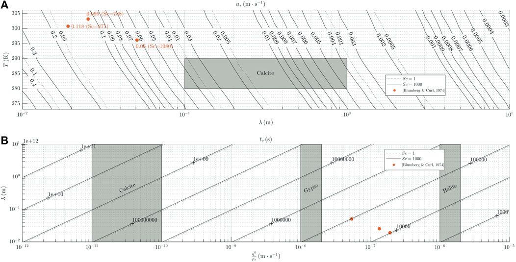
FIGURE 12. Dissolution of rocks soluble in liquid water. The shaded areas correspond to typical ranges of temperature and dissolution rates encountered in natural environments. The orange circles represent the experimental results of Blumberg and Curl (1974). (A) First law (B) Combination of second and third law.
This tool is also useful for the design of new experiments, choosing a couple (u*, T), one can then define the desired wavelength range allowing a scaling of the experiment on an adapted exposure time. We propose to design the chart for dissolution in order to obtain the exposure times of surfaces to a water flow, knowing from Eq. (9) that:
This is relevant to estimate formation time of the dissolution waves (Figure 12B) in the experiments or in natural exemples. For example, the chart does provide growth times of between 4 h and 20 h for the wavelengths obtained by Blumberg and Curl (1974). With the same wavelength and similar hydrodynamic conditions, the growth time, induced by the rate of dissolution, is therefore naturally 100 times greater for calcite than for gypsum, itself 100 times greater than for halite. Considering an average estimate of the calcite dissolution rate such that q0/ρs ≃ 4 × 10⁻¹¹ (Table 3), the chart provides a characteristic growth time of the dissolution waves of the walls of Grotte de St-Marcel of the order of ≃ 100 years. This enables an estimation of the required minimum residence time for water to form this type of beforms, but also an idea of the velocity of the paleo-flow as a function of the observed wavelength.
6 Conclusion
The development of transverse linear ablation bedforms, either by dissolution or sublimation of solid substrates, can be unified in a single analytical model that couples mass transfers and near-wall turbulent flow. The linear stability analysis of the model shows that the propagation angle, defined as the ratio between the ablation rate and the migration velocity, is equal to ≃ 60° for both ablation processes. By contrast, the coefficients of the dispersion relation differ between sublimation and ablation dissolution, because these different ablation processes involve different values of the Schmidt number. Three scaling laws derived from the model relate the geometric and kinematic characteristics of ablation waves to the characteristics of the environment in which they form: (i) bedform wavelengths are related to the ratio viscosity over friction velocity, (ii) bedform migration velocities are related to ablation rates, (iii) bedform characteristic growth times are related to viscous lengths and ablation rates. These scaling laws correctly fit a set of data measured on ablation waves on soluble rocks (by dissolution) and on volatile ices (by sublimation) in terrestrial, extra-terrestrial and experimental settings. They can be used to predict flow velocities, ablation rates and characteristic growth times for other ablation waves. Specific charts derived from the laws allow the model predictions to be used to design new experiments and to be extended to other terrestrial and planetary ablation waves.
Data availability statement
The original contributions presented in the study are included in the article/supplementary material, further inquiries can be directed to the corresponding author.
Author contributions
As a physicist, SC has proposed a unified model for the scaling laws for ablation waves in sublimation and dissolution based on the modeling of the coupled equations developed by MB. As a planetary geomorphologist, OB has contributed to find natural examples of sublimation and dissolution waves in order to validate the model. He has conducted the field trip expedition in the Saint Marcel cave. All authors contributed to the article and approved the submitted version.
Funding
TelluS programme of the INSU (CNRS) SYSTER Action 2019, in the framework of the project “Characterisation and modelling of periodic dissolution forms on limestone walls subjected to water flows”. National Planetology Plan programme of the INSU (CNRS) Action 2021, in the framework of the project “OnDiNE” that aim to design specific charts for sublimation waves experiments. This project has been supported by the Observatory of the sciences of the Universe Nantes Atlantique (Osuna, Nantes University, CNRS UAR-3281, UGE, CNAM, univ Angers, IMT Atlantique) and Région Pays de la Loire.
Acknowledgments
We acknowledge Delphine Dupuy, in charge of preservation and valorization of cultural heritage at the Saint Marcel’s cave, France; Stéphane Bonnet (GET, Toulouse, France) and Marion Massé (LPG, Nantes, France) for LIDAR acquisition in the cave; we acknowledge for scientific discussions Philippe Claudin (PMMH, Paris, France) and “les Treilles, atelier dunes” Team. We acknowledge the reviewers for their constructive feedbacks that allow to improve significantly the clarity and quality of the manuscript.
Conflict of interest
The authors declare that the research was conducted in the absence of any commercial or financial relationships that could be construed as a potential conflict of interest.
Publisher’s note
All claims expressed in this article are solely those of the authors and do not necessarily represent those of their affiliated organizations, or those of the publisher, the editors and the reviewers. Any product that may be evaluated in this article, or claim that may be made by its manufacturer, is not guaranteed or endorsed by the publisher.
References
Allen, J. R. (1971). Transverse erosional marks of mud and rock: Their physical basis and geological significance. Sediment. Geol. 5, 167–385. doi:10.1016/0037-0738(71)90001-7
Altwegg, K., Balsiger, H., Bar-Nun, A., Berthelier, J. J., Bieler, A., Bochsler, P., et al. (2015). Cometary science. 67P/Churyumov-Gerasimenko, a Jupiter family comet with a high D/H ratio. Science 347, 1261952. doi:10.1126/science.1261952
Anderson, J. D., Lau, E. L., Sjogren, W. L., Schubert, G., and Moore, W. (1996). Gravitational constraints on the internal structure of Ganymede. Nature 384, 541–543. doi:10.1038/384541a0
Banks, M. E., Byrne, S., Galla, K., McEwen, A. S., Bray, V. J., Dundas, C. M., et al. (2010). Crater population and resurfacing of the Martian north polar layered deposits. J. Geophys. Res. E Planets 115, E08006. doi:10.1029/2009JE003523
Bertrand, T., Forget, F., Umurhan, O. M., Grundy, W. M., Schmitt, B., Protopapa, S., et al. (2018). The nitrogen cycles on Pluto over seasonal and astronomical timescales. Icarus 309, 277–296. doi:10.1016/j.icarus.2018.03.012
Bertrand, T., Forget, F., Umurhan, O. M., Moore, J. M., Young, L. A., Protopapa, S., et al. (2019). The CH 4 cycles on Pluto over seasonal and astronomical timescales. Icarus 329, 148–165. doi:10.1016/j.icarus.2019.02.007
Bertrand, T., Forget, F., White, O., Schmitt, B., Stern, S. A., Weaver, H. A., et al. (2020). Pluto’s beating heart regulates the atmospheric circulation: Results from high-resolution and multiyear numerical climate simulations. J. Geophys. Res. Planets 125, e2019JE006120. doi:10.1029/2019je006120
Bertrand, T., Lellouch, E., Holler, B., Young, L., Schmitt, B., Marques Oliveira, J., et al. (2022). Volatile transport modeling on triton with new observational constraints. Icarus 373, 114764. doi:10.1016/j.icarus.2021.114764
Bintanja, R. (1999). On the glaciological, meteorological, and climatological significance of antarctic blue ice areas. Rev. Geophys. 37, 337–359. doi:10.1029/1999RG900007
Bintanja, R., Reijmer, C. H., and Hulscher, S. J. (2001). Detailed observations of the rippled surface of Antarctic blue-ice areas. J. Glaciol. 47, 387–396. doi:10.3189/172756501781832106
Blumberg, P. N., and Curl, R. L. (1974). Experimental and theoretical studies of dissolution roughness. J. Fluid Mech. 65, 735–751. doi:10.1017/S0022112074001625
Bordiec, M., Carpy, S., Bourgeois, O., Herny, C., Massé, M., Perret, L., et al. (2020). Sublimation waves: Geomorphic markers of interactions between icy planetary surfaces and winds. Earth-Science Rev. 211, 103350. doi:10.1016/j.earscirev.2020.103350
Byrne, S., and Ingersoll, A. P. (2003). A sublimation model for martian South Polar ice features. Science 299, 1051–1053. doi:10.1126/science.1080148
Byrne, S. (2009). The polar deposits of mars. Annu. Rev. Earth Planet. Sci. 37, 535–560. doi:10.1146/annurev.earth.031208.100101
Carroll, M. (2019). “Ceres: The first known ice dwarf planet,” in Ice worlds of the solar system (Berlin, Germany: Springer). doi:10.1007/978-3-030-28120-5_4
Chapman, S., Cowling, T. G., Burnett, D., and Cercignani, C. (1990). The mathematical theory of non-uniform gases: An account of the kinetic theory of viscosity, thermal conduction and diffusion in gases. Cambridge, UK: Cambridge Mathematical Library, Cambridge University Press.
Chittenden, J. D., Chevrier, V., Roe, L. A., Bryson, K., Pilgrim, R., and Sears, D. W. G. (2008). Experimental study of the effect of wind on the stability of water ice on Mars. Icarus 196, 477–487. doi:10.1016/j.icarus.2008.01.016
Claudin, P., Durán, O., and Andreotti, B. (2017). Dissolution instability and roughening transition. J. Fluid Mech. 832, R2–832R214. doi:10.1017/jfm.2017.711
Colombani, J., and Bert, J. (2007). Holographic interferometry study of the dissolution and diffusion of gypsum in water. Geochimica Cosmochimica Acta 71, 1913–1920. doi:10.1016/j.gca.2007.01.012
Conway, S. J., Hovius, N., Barnie, T., Besserer, J., Le Mouélic, S., Orosei, R., et al. (2012). Climate-driven deposition of water ice and the formation of mounds in craters in Mars’ north polar region. Icarus 220, 174–193. doi:10.1016/j.icarus.2012.04.021
Courrech du Pont, S., Narteau, C., and Gao, X. (2014). Two modes for dune orientation. Geology 42, 743–746. doi:10.1130/G35657.1
Cruikshank, D. P., Howell, R., Geballe, T., and Fanale, F. (1985). “Sulfur dioxide ice on Io,” in Ices in the solar system. Editor J. Klinger (Netherlands: Springer), 805–815. chap. Cruikshank. doi:10.1007/978-94-009-5418-2_55
Cubillas, P., Köhler, S., Prieto, M., Causserand, C., and Oelkers, E. H. (2005). How do mineral coatings affect dissolution rates? An experimental study of coupled CaCO3 dissolution - CdCO3 precipitation. Geochimica Cosmochimica Acta 69, 5459–5476. doi:10.1016/j.gca.2005.07.016
Daupley, X., Laouafa, F., Billiotte, J., and Quintard, M. (2015). “La dissolution du gypse: Quantifier les phénomènes,” in Mines and carrières hors-série, 35–43.
Deutsch, A. N., Neumann, G. A., and Head, J. W. (2017). New evidence for surface water ice in small-scale cold traps and in three large craters at the north polar region of Mercury from the Mercury Laser Altimeter. Geophys. Res. Lett. 44, 9233–9241. doi:10.1002/2017GL074723
Dougherty, M., Khurana, K., Neubauer, F., Russell, C. T., Saur, J., Leisner, J., et al. (2006). Identification of a dynamic atmosphere at Enceladus with the cassini magnetometer. Science 311, 1406–1409. doi:10.1126/science.1120985
Durán, O., Andreotti, B., Claudin, P., and Winter, C. (2019). A unified model of ripples and dunes in water and planetary environments. Nat. Geosci. 12, 345–350. doi:10.1038/s41561-019-0336-4
Eke, V. R., Lawrence, D. J., and Teodoro, L. F. (2017). How thick are Mercury’s polar water ice deposits? Icarus 284, 407–415. doi:10.1016/j.icarus.2016.12.001
Ernst, C. M., Chabot, N. L., and Barnouin, O. S. (2018). Examining the potential contribution of the hokusai impact to water ice on Mercury. J. Geophys. Res. Planets 123, 2628–2646. doi:10.1029/2018JE005552
Fanale, F. P., Postawko, S. E., Pollack, J. B., Carr, M. H., and Pepin, R. O. (1992). “Mars: Epochal climate change and volatile history,” in Mars. Editor M. George, 1135–1179.
Forget, F., Bertrand, T., Vangvichith, M., Leconte, J., Millour, E., and Lellouch, E. (2017). A post-new horizons global climate model of Pluto including the N2, CH4 and CO cycles. Icarus 287, 54–71. doi:10.1016/j.icarus.2016.11.038
Forget, F., Hourdin, F., and Dalagrand, O. (1999). Improved general circulation models of the Martian atmosphere from the surface to above 80 km. J. Geophys. Res. – Planets (E) 104, 24,155–24,175. doi:10.1029/1999JE001025
Frumkin, A. (1994). Hydrology and denudation rates of halite karst. J. Hydrology 162, 171–189. doi:10.1016/0022-1694(94)90010-8
Frumkin, A. (2013). Salt karst, 6. Amsterdam, Netherlands: Elsevier Ltd. doi:10.1016/B978-0-12-374739-6.00113-5
Gallaire, F., and Brun, P. T. (2017). Fluid dynamic instabilities: Theory and application to pattern forming in complex media. Philosophical Trans. R. Soc. A Math. Phys. Eng. Sci. 375, 20160155. doi:10.1098/rsta.2016.0155
Goodchild, M., and Ford, D. C. (1972). Analysis of scallop patterns by simulation under controlled conditions: A discussion. J. Geol. 80, 121–122. doi:10.1086/627717
Grundy, W. M., Binzel, R. P., Buratti, B. J., Cook, J. C., Cruikshank, D. P., Dalle Ore, C. M., et al. (2016). Surface compositions across pluto and Charon. Science 351, aad9189. doi:10.1126/science.aad9189
Grundy, W. M., and Fink, U. (1991). A new spectrum of triton near the time of the voyager encounter. Icarus 93, 379–385. doi:10.1016/0019-1035(91)90220-N
Gulkis, S., Allen, M., Von Allmen, P., Beaudin, G., Biver, N., Bockelée-Morvan, D., et al. (2015). Cometary science. Subsurface properties and early activity of comet 67P/Churyumov-Gerasimenko. Science 347, aaa0709–6. doi:10.1126/science.aaa0709
Gunn, A., and Jerolmack, D. J. (2022). Conditions for aeolian transport in the solar system. Nat. Astron. 6, 923–929. doi:10.1038/s41550-022-01669-0
Hagedorn, B., Sletten, R. S., and Hallet, B. (2007). Sublimation and ice condensation in hyperarid soils: Modeling results using field data from victoria valley, Antarctica. J. Geophys. Res. Earth Surf. 112, F03017. doi:10.1029/2006JF000580
Hammer, O., Lauritzen, S. E., and Jamtveit, B. (2011). Stability of dissolution flutes under turbulent flow. J. Cave Karst Stud. 73, 181–186. doi:10.4311/2011JCKS0200
Hanratty, T. J. (1981). Stability of surfaces that are dissolving or being formed by convective diffusion. Annu. Rev. Fluid Mech. 13, 231–252. doi:10.1146/annurev.fl.13.010181.001311
Hayes, A. G. (2016). The lakes and seas of titan. Annu. Rev. Earth Planet. Sci. 44, 57–83. doi:10.1146/annurev-earth-060115-012247
Head, J. W., Mustard, J. F., Kreslavsky, M. A., Milliken, R. E., and Marchant, D. R. (2003). Recent ice ages on Mars. Nature 426, 797–802. doi:10.1038/nature02114
Herny, C., Massé, M., Bourgeois, O., Carpy, S., Le Mouélic, S., Appéré, T., et al. (2014). Sedimentation waves on the martian North Polar cap: Analogy with megadunes in Antarctica. Earth Planet. Sci. Lett. 403, 56–66. doi:10.1016/j.epsl.2014.06.033
Hofstadter, M. D., and Murray, B. C. (1990). Ice sublimation and rheology: Implications for the martian polar layered deposits. Icarus 84, 352–361. doi:10.1016/0019-1035(90)90043-9
Howard, A. D. (2000). The role of eolian processes in forming surface features of the martian polar layered deposits. Icarus 144, 267–288. doi:10.1006/icar.1999.6305
Incropera, F. P., Lavine, A. S., Bergman, T. L., and DeWitt, D. P. (2007). Fundamentals of heat and mass transfer. 6 edn. New York, United States: Wiley.
Ivanov, A. B., and Muhleman, D. O. (2000). The role of sublimation for the formation of the northern ice cap: Results from the mars orbiter laser altimeter. Icarus 144, 436–448. doi:10.1006/icar.1999.6304
Jakirlić, S., Manceau, R., Šarić, S., Fadai-Ghotbi, A., Kniesner, B., Carpy, S., et al. (2009). LES, zonal and seamless hybrid LES/RANS: Rationale and application to free and wall-bounded flows involving separation and swirl. Berlin, Heidelberg: Springer, 253–282. doi:10.1007/978-3-540-89956-3_11
Jakosky, B. M. (1985). The seasonal cycle of water on Mars. Space Sci. Rev. 41, 131–200. doi:10.1007/BF00241348
James, P. B., and North, G. R. (1982). The seasonal CO2 cycle on mars: An application of an energy balance climate model. J. Geophys. Res. 87, 10271–10283. doi:10.1029/JB087iB12p10271
Kaufmann, G., Gabrovšek, F., and Romanov, D. (2014). Deep conduit flow in karst aquifers revisited. Water Resour. Res. 50, 4821–4836. doi:10.1002/2014WR015314
Kauhanen, J., Siili, T., Ja, S., and Savija, H. (2008). The Mars limited area model and simulations of atmospheric circulations for the Phoenix landing area and season of operation. J. Geophys. Res. 113, E00A14. doi:10.1029/2007JE003011
Kelly, N. J., Boynton, W. V., Kerry, K. E., Hamara, D., Janes, D. M., Reddy, R. C., et al. (2007). Seasonal polar carbon dioxide frost on Mars: Co2 mass and columnar thickness distribution. J. Geophys. Res. E Planets 112, E03S07–12. doi:10.1029/2006JE002678
Khurana, K. K., Kivelson, M. G., Stevenson, D., Schubert, G., Russell, C., Walker, R. J., et al. (1998). Induced magnetic fields as evidence for subsurface oceans in Europa and Callisto. Nature 395, 777–780. doi:10.1038/27394
Kieffer, H. H., Chase, S. C., Martin, T. Z., Miner, E. D., and Palluconi, F. D. (1976). Martian North Pole summer temperatures: Dirty water ice. Sci. (New York, N.Y.) 194, 1341–1344. doi:10.1126/science.194.4271.1341
Kivelson, M. G., Khurana, K. K., Russer, C. T., Volwerk, M., Walker, R. J., and Zimmer, C. (2000). Galileo magnetometer measurements: A stronger case for a subsurface ocean at Europa. Science 289, 1340–1343. doi:10.1126/science.289.5483.1340
Knotek, S., and Jícha, M. (2014). Modeling of shear stress and pressure acting on small-amplitude wavy surface in channels with turbulent flow. Appl. Math. Model. 38, 3929–3944. doi:10.1016/j.apm.2013.11.065
Kreslavsky, M. A., and Head, J. W. (2002a). Fate of outflow channel effluents in the northern lowlands of Mars: The vastitas borealis formation as a sublimation residue from frozen ponded bodies of water. J. Geophys. Res. Planets 107, 4-1–4-25. doi:10.1029/2001JE001831
Kreslavsky, M. A., and Head, J. W. (2002b). Mars: Nature and evolution of young latitude-dependent water-ice-rich mantle. Geophys. Res. Lett. 29, 14-1–14-4. doi:10.1029/2002GL015392
Kreslavsly, M. A., and Bondarenko, N. V. (2017). Aeolian sand transport and aeolian deposits on Venus: A review. Aeolian Res. 26, 29–46. doi:10.1016/j.aeolia.2016.06.001
Kuzan, J. D., Hanratty, T. J., and Adrian, R. J. (1989). Turbulent flows with incipient separation over solid waves. Exp. Fluids 7, 88–98. doi:10.1007/BF00207300
Law, J., and Van Dijk, D. (1994). Sublimation as a geomorphic process: A review. Permafr. Periglac. Process. 5, 237–249. doi:10.1002/ppp.3430050404
Lee, C., Lewis, S. R., and Read, P. L. (2010). A bulk cloud parameterization in a Venus general circulation model. Icarus 206, 662–668. doi:10.1016/j.icarus.2009.09.017
Lellouch, E., de Bergh, C., Sicardy, B., Ferron, S., and Käufl, H.-U. (2010). Detection of co in triton’s atmosphere and the nature of surface-atmosphere interactions. A&A 512, L8. doi:10.1051/0004-6361/201014339
Li, S., Lucey, P. G., Milliken, R. E., Hayne, P. O., Fisher, E., Williams, J. P., et al. (2018). Direct evidence of surface exposed water ice in the lunar polar regions. Proc. Natl. Acad. Sci. U. S. A. 115, 8907–8912. doi:10.1073/pnas.1802345115
Lopes, R. M., Wall, S. D., Elachi, C., Birch, S., Corlies, P., Coustenis, A., et al. (2019). Titan as revealed by the cassini radar. Space Sci. Rev. 215, 33. doi:10.1007/s11214-019-0598-6
Lunine, J. I., and Atreya, S. K. (2008). The methane cycle on Titan. Nat. Geosci. 1, 159–164. doi:10.1038/ngeo125
Malin, M. C., and Edgett, K. S. (2001). Mars global surveyor mars orbiter camera: Interplanetary cruise through primary mission. J. Geophys. Res. 106, 23429,429–23570,570. doi:10.1029/2000JE001455
Manceau, R., Carpy, S., and Alfano, D. (2002). “A rescaled v2?f model: First application to separated and impinging flows,” in Engineering turbulence modelling and experiments 5. Editors W. Rodi, and N. Fueyo (Oxford: Elsevier Science Ltd), 107–116. doi:10.1016/B978-008044114-6/50009-0
Mangold, N. (2011). Ice sublimation as a geomorphic process: A planetary perspective. Geomorphology 126, 1–17. doi:10.1016/j.geomorph.2010.11.009
Massé, M., Bourgeois, O., Le Mouélic, S., Verpoorter, C., Le Deit, L., and Bibring, J. P. (2010). Martian polar and circum-polar sulfate-bearing deposits: Sublimation tills derived from the North Polar Cap. Icarus 209, 434–451. doi:10.1016/j.icarus.2010.04.017
Massé, M., Bourgeois, O., Mouélic, S. L., Verpoorter, C., Spiga, A., and Deit, L. L. (2012). Wide distribution and glacial origin of polar gypsum on Mars. Earth Planet. Sci. Lett. 317-318, 44–55. doi:10.1016/j.epsl.2011.11.035
McKinnon, W. B., Nimmo, F., Wong, T., Schenk, P. M., White, O. L., Roberts, J. H., et al. (2016). Convection in a volatile nitrogen-ice-rich layer drives Pluto’s geological vigour. Nature 534, 82–85. doi:10.1038/nature18289
Meakin, P., and Jamtveit, B. (2010). Geological pattern formation by growth and dissolution in aqueous systems. Proc. R. Soc. A Math. Phys. Eng. Sci. 466, 659–694. doi:10.1098/rspa.2009.0189
Mellor, M., and Swithinbank, C. (1989). Airfields on Antarctic glacier ice. Hanover NH: Cold Region Research and Engineering Lab. Tech. rep.
Milkovich, S. (2006). Surface textures of mars’ north polar layered deposits: A framework for interpretation and future exploration. Mars J. 21, 21–45. doi:10.1555/mars.2006.0003
Millour, E., Forget, F., Spiga, A., Vals, M., Zakharov, V., Montabone, L., et al. (2018). “The mars climate Database (version 5.3),” in Scientific workshop: “From Mars express to ExoMars” (ESAC madrid), 27–28.
Moore, J. M., Howard, A. D., Umurhan, O. M., White, O. L., Schenk, P. M., Beyer, R. A., et al. (2018). Bladed terrain on pluto: Possible origins and evolution. Icarus 300, 129–144. doi:10.1016/j.icarus.2017.08.031
Moore, J. M., Howard, A. D., Umurhan, O. M., White, O. L., Schenk, P. M., Beyer, R. A., et al. (2017). Sublimation as a landform-shaping process on Pluto. Icarus 287, 320–333. doi:10.1016/j.icarus.2016.08.025
Moores, J. E., Smith, C. L., Toigo, A. D., and Guzewich, S. D. (2017). Penitentes as the origin of the bladed terrain of tartarus dorsa on pluto. Nature 541, 188–190. doi:10.1038/nature20779
Morison, A., Labrosse, S., and Choblet, G. (2021). Sublimation-driven convection in sputnik planitia on pluto. Nature 600, 419–423. doi:10.1038/s41586-021-04095-w
Morse, J. W., and Arvidson, R. S. (2002). The dissolution kinetics of major sedimentary carbonate minerals. Earth-Science Rev. 58, 51–84. doi:10.1016/S0012-8252(01)00083-6
Ng, F. S., and Zuber, M. T. (2006). Patterning instability on the Mars polar ice caps. J. Geophys. Res. E Planets 111. doi:10.1029/2005JE002533
Nguyen, T. G., Radebaugh, J., Innanen, A., and Moores, J. E. (2020). A survey of small-scale (<50 m) surface features on the Martian north polar cap using HiRISE. Planet. Space Sci. 182, 104809. doi:10.1016/j.pss.2019.104809
Obleitner, F., and Spötl, C. (2011). The mass and energy balance of ice within the Eisriesenwelt cave, Austria. Cryosphere 5, 245–257. doi:10.5194/tc-5-245-2011
Ohmura, A. (2004). Cryosphere during the twentieth century. Geophys. Monogr. Ser. 150, 239–257. doi:10.1029/150GM19
Pankine, A. A., and Tamppari, L. K. (2015). Constraints on water vapor vertical distribution at the Phoenix landing site during summer from MGS TES day and night observations. Icarus 252, 107–120. doi:10.1016/j.icarus.2015.01.008
Pankine, A. A., Tamppari, L. K., and Smith, M. D. (2010). MGS TES observations of the water vapor above the seasonal and perennial ice caps during northern spring and summer. Icarus 210, 58–71. doi:10.1016/j.icarus.2010.06.043
Petrosyan, A., Galperin, B., Larsen, S. E., Lewis, S., Maattanen, A., Read, P. L., et al. (2011). The Martian atmospheric boundary layer. Rev. Geophys. 49. doi:10.1029/2010RG000351
Port, S. T., Chevrier, V. F., and Kohler, E. (2020). Investigation into the radar anomaly on Venus: The effect of Venus conditions on bismuth, tellurium, and sulfur mixtures. Icarus 336, 113432. doi:10.1016/j.icarus.2019.113432
Protopapa, S., Grundy, W. M., Reuter, D. C., Hamilton, D. P., Dalle Ore, C. M., Cook, J. C., et al. (2017). Pluto’s global surface composition through pixel-by-pixel Hapke modeling of New Horizons Ralph/LEISA data. Icarus 287, 218–228. doi:10.1016/j.icarus.2016.11.028
Schaefer, L., and Fegley, F. (2004). Heavy metal frost on Venus. Icarus 168, 215–219. doi:10.1016/j.icarus.2003.11.023
Schenk, P. M. (1991). Fluid volcanism on Miranda and ariel: Flow morphology and composition. J. Geophys. Res. 96, 1887–1906. doi:10.1029/90jb01604
Schmitt, B., Philippe, S., Grundy, W. M., Reuter, D. C., Côte, R., Quirico, E., et al. (2017). Physical state and distribution of materials at the surface of Pluto from New Horizons LEISA imaging spectrometer. Icarus 287, 229–260. doi:10.1016/j.icarus.2016.12.025
Scully, J. E., Russell, C. T., Yin, A., Jaumann, R., Carey, E., Castillo-Rogez, J., et al. (2015). Geomorphological evidence for transient water flow on Vesta. Earth Planet. Sci. Lett. 411, 151–163. doi:10.1016/j.epsl.2014.12.004
Skorov, Y. V., Markiewicz, W. J., Basilevsky, A. T., and Keller, H. U. (2001). Stability of water ice under a porous nonvolatile layer: Implications to the south polar layered deposits of Mars. Planet. Space Sci. 49, 59–63. doi:10.1016/S0032-0633(00)00121-5
Smith, I. B., and Holt, J. W. (2010). Onset and migration of spiral troughs on Mars revealed by orbital radar. Nature 465, 450–453. doi:10.1038/nature09049
Smith, I. B., Holt, J. W., Spiga, A., Howard, A. D., and Parker, G. (2013). The Spiral troughs of Mars as cyclic steps. J. Geophys. Res. Planets 118, 1835–1857. doi:10.1002/jgre.20142
Smith, I. B., and Spiga, A. (2018). Seasonal variability in winds in the north polar region of Mars. Icarus 308, 188–196. doi:10.1016/j.icarus.2017.10.005
Sori, M. M., Bapst, J., Becerra, P., and Byrne, S. (2019). Islands of ice on mars and pluto. J. Geophys. Res. Planets 124, 2522–2542. doi:10.1029/2018JE005861
Strobel, D. F., and Zhu, X. (2017). Comparative planetary nitrogen atmospheres: Density and thermal structures of Pluto and Triton. Icarus 291, 55–64. doi:10.1016/j.icarus.2017.03.013
Stubbs, T. J., and Wang, Y. (2012). Illumination conditions at the Asteroid 4 Vesta: Implications for the presence of water ice. Icarus 217, 272–276. doi:10.1016/j.icarus.2011.11.007
Telfer, M. W., Parteli, E. J. R., Radebaugh, J., Beyer, R. A., Bertrand, T., Forget, F., et al. (2018). Dunes on pluto. Science 360, 992–997. doi:10.1126/SCIENCE.AAO2975
Thomas, R. (1979). Size of scallops and ripples formed by flowing water. Nature 277, 281–283. doi:10.1038/277281a0
Thorness, C. B., and Hanratty, T. J. (1979). Mass transfer between a flowing fluid and a solid wavy surface. AIChE J. 25, 686–697. doi:10.1002/aic.690250415
Trowbridge, A. J., Melosh, H. J., Steckloff, J. K., and Freed, A. M. (2016). Vigorous convection as the explanation for Pluto’s polygonal terrain. Nature 534, 79–81. doi:10.1038/nature18016
van den Broeke, M. R., and Bintanja, R. (1995). Ummertime atmospheric circulation in the vicinity of a blue ice area in Queen Maud Land, Antarctica. Boundary-Layer Meteorol. 72, 411–438. doi:10.1007/BF00709002
Weller, G. (1969). The heat and mass balance of snow dunes on the central Antarctic plateau. J. Glaciol. 8, 277–284. doi:10.3189/S0022143000031257
White, O. L., Moore, J. M., McKinnon, W. B., Spencer, J. R., Howard, A. D., Schenk, P. M., et al. (2017). Geological mapping of sputnik planitia on pluto. Icarus 287, 261–286. doi:10.1016/j.icarus.2017.01.011
Keywords: sublimation, dissolution, instability, scaling laws, morphological markers, comparative planetology, ablation waves
Citation: Carpy S, Bordiec M and Bourgeois O (2023) Scaling laws for ablation waves formed by ice sublimation and rock dissolution: applications to the Earth, Mars and Pluto. Front. Astron. Space Sci. 10:1176158. doi: 10.3389/fspas.2023.1176158
Received: 28 February 2023; Accepted: 13 April 2023;
Published: 30 May 2023.
Edited by:
Fulvio Franchi, Botswana International University of Science and Technology, BotswanaCopyright © 2023 Carpy, Bordiec and Bourgeois. This is an open-access article distributed under the terms of the Creative Commons Attribution License (CC BY). The use, distribution or reproduction in other forums is permitted, provided the original author(s) and the copyright owner(s) are credited and that the original publication in this journal is cited, in accordance with accepted academic practice. No use, distribution or reproduction is permitted which does not comply with these terms.
*Correspondence: Sabrina Carpy, c2FicmluYS5jYXJweUB1bml2LW5hbnRlcy5mcg==
†These authors have contributed equally to this work