 Brandon L. Burkholder1,2*
 Li-Jen Chen2
 Kareem Sorathia3
 Anthony Sciola3
 Slava Merkin3Karlheinz J. Trattner4Daniel Gershman2
 Xuanye Ma5
 Hyunju Connor2
- 1University of Maryland Baltimore Country, Baltimore, MD, United States
- 2NASA Goddard Space Flight Center, Greenbelt, MD, United States
- 3Johns Hopkins University Applied Physics Laboratory, Laurel, MD, United States
- 4Laboratory of Atmospheric and Space Physics, University of Colorado, Boulder, CO, United States
- 5Center for Space and Atmospheric Research, Embry-Riddle Aeronautical University, Daytona Beach, FL, United States
High-resolution global magnetohydrodynamics (MHD) simulations include both meso- and global-scale processes occurring at the magnetopause, which interact to determine the time-dependent orientation of the day-side x-line (DXL). This study demonstrates that the global orientation of the DXL in GAMERA global MHD simulations varies on a time scale of minutes during steady southward interplanetary magnetic field conditions. This behavior manifests in observational data when reconnection outflows indicate that the direction to the x-line is opposite to the prediction from a steady-state model of the reconnection location. Because steady-state models of the DXL do not capture dynamics that are independent of solar wind variations, particularly surface waves and flux transfer events, they represent a time-averaged state of the system.
1 Introduction
At the day-side magnetopause, magnetic reconnection changes the topology of magnetic fields on adjacent sides of the boundary to create open magnetic field lines, leading to energy and momentum fluxes into the magnetosphere. The resulting space weather phenomena are dependent on where and how much of the solar wind is allowed to flow into the magnetosphere. Therefore, the location and extent of the day-side reconnection site at Earth’s magnetopause is a fundamentally important problem in space physics. In previous work, multi-spacecraft conjunctions at the magnetopause have observed an extended day-side x-line (Peterson et al., 1998; Phan et al., 2000; Dunlop et al., 2011), in addition to IMAGE observations (Fuselier et al., 2002), but these could not directly observe its orientation. In-situ measurements near the magnetopause observe accelerated flows that can be used to estimate the distance from the spacecraft to the x-line (e.g., Gosling et al., 1990; Swisdak and Drake, 2007), and radar observations of fast flow channels have also been used to determine the x-line location and extent (Pinnock and Rodger, 2000). Scurry et al. (1994) examined accelerated flow events in ISEE 2 observations at the magnetopause and found their location and direction indicates that merging occurs most often near the subsolar point along a line of length
Not accounted for in any of these models is the time-dependent shape of the magnetopause boundary. For instance, flux tubes generated by reconnection being dragged along the magnetopause (Russell and Elphic, 1978), the Kelvin-Helmholtz instability (KHI) and surface waves (Ong and Roderick, 1972; Pu and Kivelson, 1983; Plaschke et al., 2013), in addition to warping (Jacobsen et al., 2009; Chen et al., 2021a) and any other dynamics of the boundary, are interacting at the magnetopause. In particular, the interaction of reconnection and KH has been studied extensively. Nykyri and Otto (2001, 2004) showed that filamentary currents are generated in the KHI which can lead to reconnection, and Ma et al. (2014a,b) discussed the opposing cases of KH initiated by reconnection and reconnection initiated by KH.
Each individual dynamical process on the magnetopause boundary may have a predictable effect on the global x-line structure, but when they occur simultaneously it is the interaction that leads to observed time dynamics of the DXL. Understanding these dynamics is vital because often we want to determine the distance to the x-line at the location of a spacecraft at a single instance in time (e.g., Souza et al. (2017) among others). Modern global magnetosphere simulations have the ability to capture both meso- (1 to a few RE) and global-scale processes (Sorathia et al., 2020) that interact to determine the orientation of the x-line, which has the potential to provide a better prediction of the global x-line orientation for any given solar wind conditions.
This paper is organized as follows. In section 2, we examine Magnetospheric Multiscale (MMS) data during steady southward IMF near the magnetopause boundary and compare the direction of observed reconnection outflows with the maximum magnetic shear model. Section 3 provides a description of the simulation model and observations from synthetic spacecraft. Section 4 explores the time dynamics of the three-dimensional global DXL during steady solar wind driving. Section 5 explores specific processes on the magnetopause boundary which lead to the time-dependence of the global DXL. Section 6 provides a discussion and summary of conclusions.
2 MMS observations
Figure 1 presents an overview (with all vector quantities in GSM coordinates) of two magnetopause boundary crossings by the MMS1 spacecraft. Event 1 (Figures 1A–F) occurred along the dawn flank and above the GSM equator. The local magnetosheath magnetic field [Figure 1A, observed by the MMS FGM instrument (Russell et al., 2016)] between the vertical dashed lines is strongly southward with Bx and By both undergoing a change of sign. The magnetopause boundary is encountered just after the vertical dashed lines, around 11:04 UT, as is evident in the ion energy spectrogram [Figure 1C, ion observations from the Fast Plasma Investigation Pollock et al. (2016)] and ion density (Figure 1D). Event 2 (Figure 1G–L) occurred in the post-noon sector and near the GSM equator. Between the vertical dashed black lines the magnetic field (Figure 1G) is strongly southward with a significant Bx component. The ion energy spectrogram (Figure 1I) and ion density (Figure 1J) indicate the magnetopause is encountered at 10:22 UT, just after the vertical dashed lines.
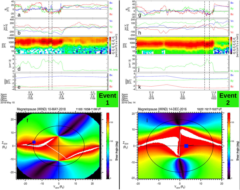
FIGURE 1. MMS observations of accelerated ion flows near the magnetopause boundary with strongly southward local magnetic field (between vertical dashed lines). Event 1 is given in (A-F) and Event 2 is given in (G-L). The time series panels are from top to bottom: magnetic field, ion velocity, ion energy spectrogram, ion density, OMNIWeb IMF (all vector quantities are in GSM coordinates). Panels (F,L) show the maximum magnetic shear model outputs for Events 1 and 2, respectively. The blue square shows the position of MMS and the observed ion velocity is directed along the black line emanating from the spacecraft.
Between the vertical dashed black lines, Figures 1B, H show accelerated ion flows tangent to the magnetopause where the local magnetic field (Figures 1A, G) is strongly southward. Furthermore, the OMNIWeb data service indicates at the bow shock nose the IMF has a steady Bz,sw < 0 for both events (Figures 1E, K). The vertical dashed lines enclose vz < − 100 km/s for Event 1 and vz > 50 km/s for Event 2. These are larger than the typical velocity fluctuations occurring in the low-latitude terrestrial magnetosheath. The strong vy during both events corresponds to the local magnetosheath flow being deflected around the magnetopause. To test whether the fast vz flows have a reconnection source, the Walén relation (Sonnerup et al., 1987; 1995) was applied. All data were interpolated to the FPI fast mode time resolution (dt = 4.5 s) and Δf(t) = (|f (t −dt) − f (t +dt)| + |f(t) − f (t −dt)| + |f(t) − f (t + dt)|)/3 is calculated at each time t, where f is either the observed vz or
The maximum magnetic shear model outputs (Trattner et al., 2007; Trattner et al., 2021) for Events 1 and 2 are shown in Figures 1F, L, respectively. The color represents the magnetic shear angle of IMF draped over the magnetopause boundary and the blue square is the location of MMS, with a black line pointing in the direction of the observed ion velocity. The region of largest magnetic shear angle at each local time (colorbar saturates to white) is the predicted location of the DXL. For Event 1 (Figure 1F), at the local time corresponding to MMS, the x-line is about 2 RE below the spacecraft, which would suggest reconnection outflows should be directed in the positive z-direction at MMS, while the observed fast vz is actually negative (Figure 1B between vertical dashed lines). Similarly, Event 2 shows at the local time corresponding to the location of MMS, the DXL is about 5 RE above the spacecraft, suggesting reconnection outflows should be directed in the negative z-direction at MMS, while the observed fast vz is positive (Figure 1B between vertical dashed lines). For the case of Event 2, it is known that the maximum magnetic shear model does not handle a significant Bx well, which could be why the difference is much larger than Event 1. Scurry et al. (1994) found a few similar accelerated flow events, mostly which were attributed to reconnection away from the day-side equator and a “sporadic merging pattern.” The interpretation of these fast flows on the magnetosheath side of the magnetopause boundary is that they are associated with reconnection sites that are displaced from the expected location based on a steady-state model of the magnetopause boundary. In the following sections, it is demonstrated that the time-dependent orientation of the DXL during steady southward IMF can explain the observed reconnection outflows.
3 Simulation model
Grid Agnostic MHD for Extended Research Applications (GAMERA) is a general purpose finite volume solver for the ideal equations of MHD (Zhang et al., 2019). Applied to the global terrestrial magnetosphere, its predecessor, the Lyon-Fedder-Mobarry (LFM) simulation (Lyon et al., 2004), has been extremely successful. GAMERA was designed for massively parallel execution to reach very high resolution and also can be coupled with other magnetospheric modules to include different physics (Lin et al., 2021; Pham et al., 2022).
GAMERA utilizes a warped spherical grid with highest resolution near the day-side magnetopause. Simulations in this paper use a QUAD (OCT) resolution grid with 96 × 96 × 128 (192 × 192 × 256) cells in the radial, polar, and azimuthal directions. The grid covers from 25 RE upwind of the subsolar point to 300 RE down the magnetotail. The spherical inner boundary at 2 RE is coupled to a two-dimensional, integrated ionospheric model, the RE-developed Magnetosphere-Ionosphere Coupler/Solver (REMIX), a rewrite of the MIX code (Merkin and Lyon, 2010). REMIX solves Ohm’s law in the ionosphere using the MHD field-aligned currents and a tensor of height-integrated ionospheric conductivities (Fedder and Lyon, 1995; Zhang et al., 2015). Simulations in this paper have no coupling to an inner magnetosphere convection module. The GAMERA-REMIX geospace model is solved in the SM coordinate frame. This system has the Z-axis parallel to the magnetic dipole axis (positive North) and its Y-axis perpendicular to the plane containing the dipole axis and the Earth-Sun line (positive in the direction opposite to Earth’s orbit). To compare QUAD and OCT resolution, both grids were re-sampled onto the same regular Cartesian grid with spacing 0.1 RE.
In examining the orientation of the DXL, it is important to note that the version of GAMERA used in this study is an MHD model where numerical resistivity breaks the frozen-in condition, allowing reconnection to occur. This means the resistivity sets in when and where the current sheet collapses to the grid scale. Ouellette et al. (2010) used GAMERA and found during northward IMF that the reconnection location was not the same as OpenGGCM simulations using an explicit constant resistivity (Dorelli et al., 2007). Explicit resistivity is an available option for the GAMERA simulations, as Arnold et al. (2023) used a data-inferred resistivity to incite reconnection in empirically-specified locations. But, a reason to favor the numerical resistivity for this study is that the highest resolution in these simulations is
This study utilizes 4 simulations. The magnetosphere is driven by a constant solar wind directed purely in the x-direction and with a density of 5 cm−3. For 3 of the 4 simulations, vx = −400 km/s, and vx = −550 km/s for the other. Each simulation underwent the same 6 h preconditioning period: the IMF is directed purely southward (Bz = −5 nT) for 2 h, purely northward (Bz = 5 nT) for 2 h, then purely southward again for 2 more hours (Merkin et al., 2013; Wiltberger et al., 2015; Sorathia et al., 2019). After preconditioning, the simulation runs for 2 additional hours with purely southward IMF for 3 of the 4 simulations, and [By,Bz] = [1.0,-4.9] nT (clock angle 169°) for the other (note |B| = 5 nT for all simulations). The analysis begins after t = 8 h and as a shorthand we will, for example, refer to 8:05 as t = 5 min. Throughout the simulation, dipole tilt is zero and the F10.7 index is 100, which determines the Pedersen and Hall conductances. The four simulations, which will be hereafter referred to as one to four, are shown in Table 1.

TABLE 1. Parameters for GAMERA global MHD simulations.
Figure 2 shows observations from synthetic satellites placed on the magnetopause of simulation 2. Figure 2A gives a snapshot of three-dimensional magnetic field lines (blue: closed magnetosphere, red: magnetopause boundary layer). Four synthetic spacecraft (green stars) observe the magnetopause boundary, at y-z coordinates [-5,0], [0,-1.5], [0,1.5], [5,0], with x-coordinates to place them within the primary reconnection exhaust. Since the simulation has undergone steady driving with a southward IMF for sufficient time to reach a steady state, the day-side magnetopause standoff distance is constant and the spacecraft are kept stationary. Figures 2B–D show the observed time series of vz from the synthetic satellites. At each location, the direction of vz changes multiple times over the course of 1-h constant solar wind driving. This demonstrates that the simulation x-line wanders above and below the spacecraft (and therefore equator plane), even when the IMF is steadily southward. A real satellite would not be able to linger at the magnetopause, but Figure 2 demonstrates that the observations in Figure 1 could indeed be indicating the direction to the x-line at the local time of MMS is opposite to what is predicted by the maximum magnetic shear model.
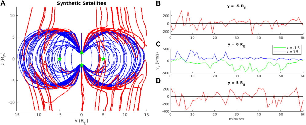
FIGURE 2. (A) Synthetic satellite (green stars) positions (y-z plane) on the magnetopause boundary in a GAMERA global MHD simulation with purely southward IMF. Blue magnetic field lines are closed magnetospheric flux and red field lines are magnetopause boundary, mapping to the inner boundary of the simulation at one end only. (B–D) 1-h synthetic satellite observations of vz, showing sign changes that indicate the x-line moving above and below the position of each satellite.
4 Global day-side X-line
Figure 3 illustrates a single snapshot of the DXL for simulations 1 (left) and 2 (right) at the same simulation time (t = 51 min, chosen arbitrarily). In the top row, the fully three-dimensional magnetopause is colored by the magnetic shear angle, and viewed in the y-z plane. The shear angle is calculated by defining the magnetopause surface as the magnetic field line open/closed boundary, then taking the shear angle between the magnetic field vectors at 0.1 RE inwards and outwards from the surface along the normal direction. The choice of 0.1 RE is not motivated by any predicted boundary width but by the simulation resolution. Field lines are traced using built-in Matlab stream line tracing, which has been verified against the native GAMERA field line tracer (Sorathia et al., 2017). This approach reveals the detailed structure of the DXL (compared with, for example, Connor et al. (2015), where the shear angle was calculated from the magnetic fields at two points 3 RE inward and outward from the magnetopause along radial lines).
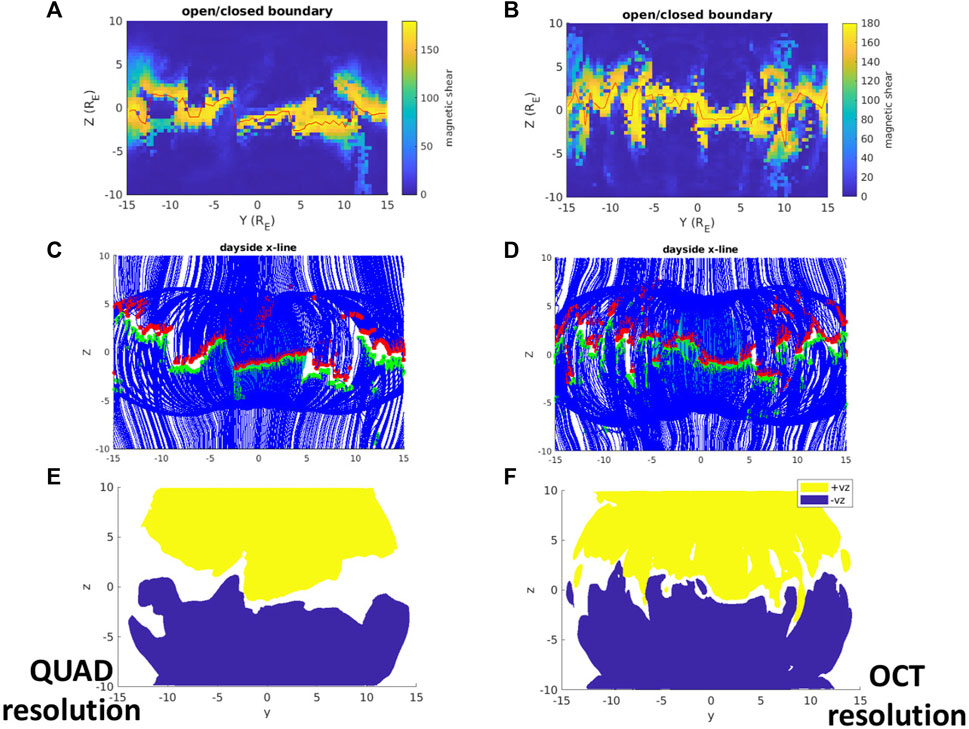
FIGURE 3. Visualizations of the day-side x-line during purely southward IMF at different simulation resolutions. Top row (A,B) shows the magnetic shear angle across the three-dimensional magnetopause boundary, viewed from the y-z plane. Middle row (C,D) shows the magnetic field reversal at the day-side x-line (red and green dots show the Bz reversal on field lines originating from the northern and southern cusps, respectively). Bottom row (E,F) shows ± 100 km/s vz contours (reconnection outflows). See the main text for more description on how these visualizations are constructed. Left column is simulation 1 and right column is simulation 2, at t = 51 min for both cases.
Of course, a large shear angle does not guarantee that reconnection is occurring at that location, but it is one indicator. In the second row of Figure 3, a large number of three-dimensional blue field lines are traced, each of which belongs to the cusp. These cusp field lines are located by covering a sphere with radius 5 RE in field lines. The open-closed boundary is determined on those field lines and then only those which are open and immediately adjacent to closed field are plotted, i.e., they are the most recently reconnected/first open field lines, having northward Bz on the magnetosphere side and southward Bz on the magnetosheath side. For field lines originating from the southern (northern) hemisphere, a green (red) marker is plotted where the z-component reverses direction, i.e., where Bz = 0. This presents a picture of the DXL by showing the magnetic topology of the most recently reconnected field lines (Laitinen et al., 2006; Mejnertsen et al., 2021). The day-side magnetic field lines reveal piece-wise x-line segments similar to the x-line structure found in the Gorgon MHD code for relatively steady strongly southward IMF (Mejnertsen et al., 2021), which were attributed to flux rope formation due to multiple reconnection sites on the magnetopause, as discussed by Fuselier et al. (2019) and others. In the second row of Figure 3, the magnetic field reversals agree with the detailed structure of magnetic shear angle (first row), suggesting there is reconnection occurring almost everywhere that the shear angle is close to 180°.
To confirm that reconnection is actively operating, the final row of Figure 3 shows fully three-dimensional contours of vz viewed in the y-z plane. The yellow contour encloses velocities greater than 100 km/s and the blue contour encloses velocities less than −100 km/s. The notable feature is where the flow reverses, forming a thin band of white between the yellow and blue contours. The flow reversal shows that the orientation of the x-line at this time step is indeed traced out by the regions of largest magnetic shear. A comparison of the different simulation resolutions reveals that the structure of the x-line is not converging with higher resolution (at any single time-step). This is not surprising, since the dynamics of interest are occurring during constant IMF orientation. The important result is that both resolutions show the same type of structure qualitatively, confirming that the existence of these structures is independent of the simulation resolution. Note also that we have only characterized the x-line to y = ±15 RE, and leave the tail-ward flank regions for future study.
This highly-structured DXL revealed by the global MHD simulation is different from a simplified picture during purely southward IMF and zero dipole tilt, where the x-line would form a continuous and smooth arc having southward (northward) directed reconnection exhausts in the southern (northern) hemisphere. The flow contours in Figures 3E, F provide an explanation for why the observations in Figure 1 are not in agreement with the maximum magnetic shear model for those events. Furthermore, the time dynamics of the x-line explain the synthetic satellite observations in Figure 2. A 1-h movie with 1-min output cadence of the magnetopause magnetic shear angle is included in the Supplementary Material to demonstrate these dynamic structures for each simulation. The results suggests that a “simple” x-line is not stable for steady southward IMF. This is not surprising, as Raeder (2006) examined in detail how x-lines in global MHD simulation become unstable. This was also predicted by the analytical considerations of Lau and Finn (1990), who noted, based on the null point analysis by Greene (1988), that a continuum of nulls is not structurally stable.
5 Length of the x-line and physical process responsible for magnetopause structure
The top row of Figure 4 shows the maximum magnetic shear model (Trattner et al., 2007; Trattner et al., 2021) with zero dipole tilt for IMF clock angles of 180° (left) and 169° (right). The x-line length can be measured in the y-z plane by tracing across the region of largest magnetic shear (light grey line). For purely southward IMF the x-line runs straight across the magnetopause, with a length of 30 RE between y = −15 and 15 RE (neglecting magnetopause curvature) that is fixed in time if the IMF does not change. The 169° clock angle IMF has a slightly larger length of
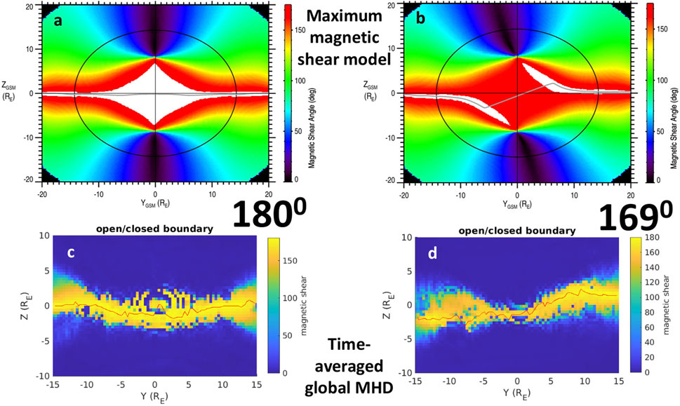
FIGURE 4. Top row (A,B) shows the maximum magnetic shear model (Trattner et al., 2007; Trattner et al., 2021) for 180°(A) and 169°(B) clock angle IMF, with zero dipole tilt and Bx. The light grey curve traces the maximum magnetic shear angle across the magnetopause. Bottom panels (C,D) show the magnetic shear angle across the magnetopause for simulations 2 (C) and 4 (D) time-averaged over 1 h. Time-averaged simulation 2 (4) has an X-line length (red line tracing the maximum magnetic shear angle across the simulation magnetopause projected onto the y-z plane) between y = −15 and y = 15 RE that is 39 (37) RE.
Shown in Figures 4C, D is the orientation of the x-line from 1 h time-averages of simulations 2 (left) and 4 (right). The thin red line is drawn in the y-z plane through the maximum value of magnetic shear angle from y = −15 to y = 15 RE. The length of this curve is 39 (37) RE for simulation 2(4). The x-line length in simulation 2 is significantly longer than the estimate from the 180° maximum magnetic shear model. However that estimate is based on a straight line whereas the maximum magnetic shear model actually shows 180° shear angles far from the equator at local times near noon. Thus the maximum magnetic shear model (in a time-averaged sense) does not rule out the type of time-dependent behavior that the simulation exhibits (large shear angles can be significantly separated from the equatorial plane). In the time-averaged simulation 4 (Figure 4D), the x-line orientation agrees well with the maximum magnetic shear model, and the length is well-captured by the red trace, with few fluctuations that artificially increase the x-line length. The two examples in Figure 4 illustrate that the maximum magnetic shear model represents a time averaged state of the magnetic shear on the magnetopause surface. This is because it does not take into account any magnetopause dynamics in the same way that time averaging the simulation smooths out meso-scale structures. For the single time-steps in Figure 3, the x-line lengths (see thin red line in Figures 3A, B) are 63 and 80 RE in simulations 1 and 2, respectively. These lengths are tracing out the large scale structure of the DXL that exists at a single instance of time. Note also that it is only possible to clearly define a length of the x-line using the magnetic shear angle in the simulation because of the symmetry in the system for strongly southward IMF orientations. When component reconnection operates it is no longer possible to define the length of the x-line, since reconnection occurs over a large area of the magnetopause not concentrated along a single line.
Figure 5 demonstrates the time-dependence of the simulation x-line length. The 2-dimensional magnetic shear angle maps used to calculate these lengths were computed at a finite resolution of 0.4 RE to minimize any effect of the “coastal paradox.” The length of the x-line from y = −15 to y = 15 RE and projected into the y-z plane is plotted as a function of time with solid lines for simulations 1–4 (red, green, blue, black, respectively), along with a constant value of 39 RE from the time-averaged simulation 2 (magenta). The time-dependent structure of the x-line means that sometimes its length can be greater than 90 RE. There are also times when a single time-step of the simulation has an x-line length similar to the time-averaged simulation, but it is never any smaller by a significant amount. From one time-step to the next, a time scale of 1-min, the length of the x-line can change by 20 RE. Since the length is computed between fixed y-coordinates at −15 and 15 RE, it is essentially a measure of the complexity.
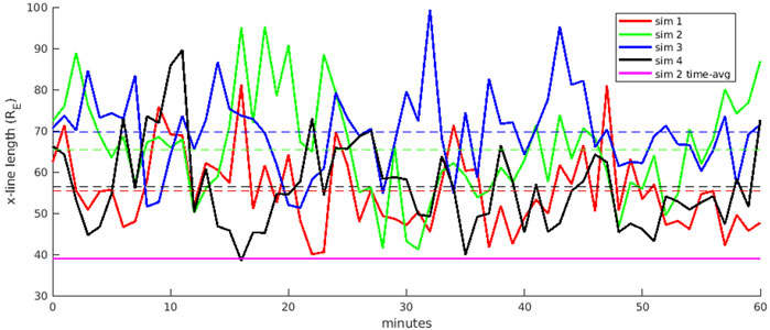
FIGURE 5. Solid lines give the length of the day-side x-line between y = −15 and y = 15 RE as a function of time for 1 h (see legend for simulation colors). Dashed lines are the 1-h average of the correspondingly colored solid line. Magenta line is the x-line length from a 1-h time average of simulation 2.
Over the entire hour, the average x-line length for each simulation is plotted as a dashed line in corresponding colors. Note this is different than the solid magenta line, which is the x-line length of the time-averaged simulation, rather than average length of the x-line over time. Simulation 1 has the smallest average and simulation 3 the largest. The simulation 2 average is greater than simulation 1 but less than simulation 3, leading to the conclusion that higher solar wind velocity produces more complexity in the DXL. With an average length of 56 RE, Figure 5 also shows that simulation 4 has a less complex x-line compared to simulation 2, leading to the conclusion that the small component of By has a stabilizing effect. The time-dependent structures that produce these variations in the x-line length are flux ropes and surface waves, which will be demonstrated in Figures 6–8.
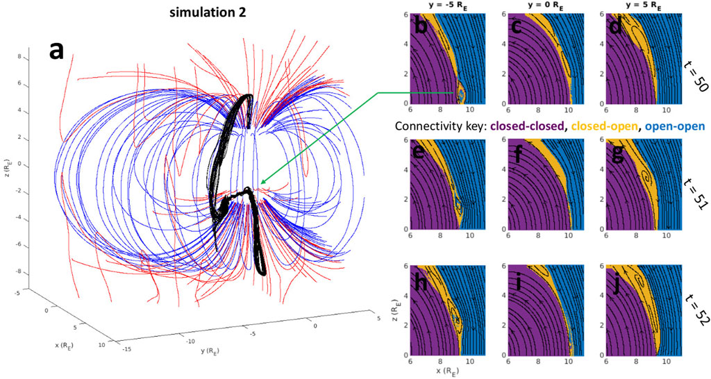
FIGURE 6. (A) Three-dimensional magnetic field lines from simulation 2 at t = 50. Blue: closed magnetosphere (connected at both ends to the inner boundary), red: magnetopause boundary layer (connected at one end to the inner boundary), black: closed magnetic field flux rope core. (B–J) Magnetic connectivity maps in 3 different y-cuts and 3 different simulation times for simulation 2. The connectivity key is given with color-matching text. Black magnetic field lines are traced in the plane for context.
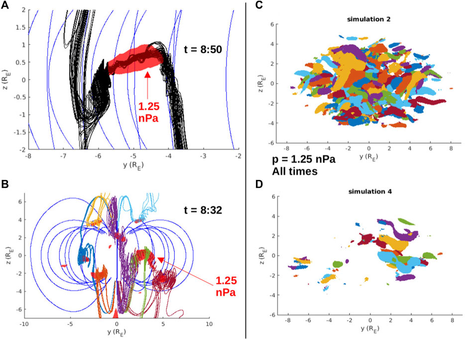
FIGURE 7. (A) Zoom-in view of closed flux rope from Figure 6A, with red thermal pressure contour enclosing p > 1.25 nPa. (B) Simulation snapshot at t = 32 min showing multiple flux rope structures with different magnetic topologies on the magnetopause boundary. Each flux rope is associated with a red contour enclosing p > 1.25 nPa. Panels (C) and (D) show the contours p > 1.25 nPa (with arbitrary colors) from each output during the 1-h steady driving interval in simulations 2 and 4, respectively. There are the same number of outputs so the larger number of contours in (C) indicates more flux rope activity over the 1-h interval.
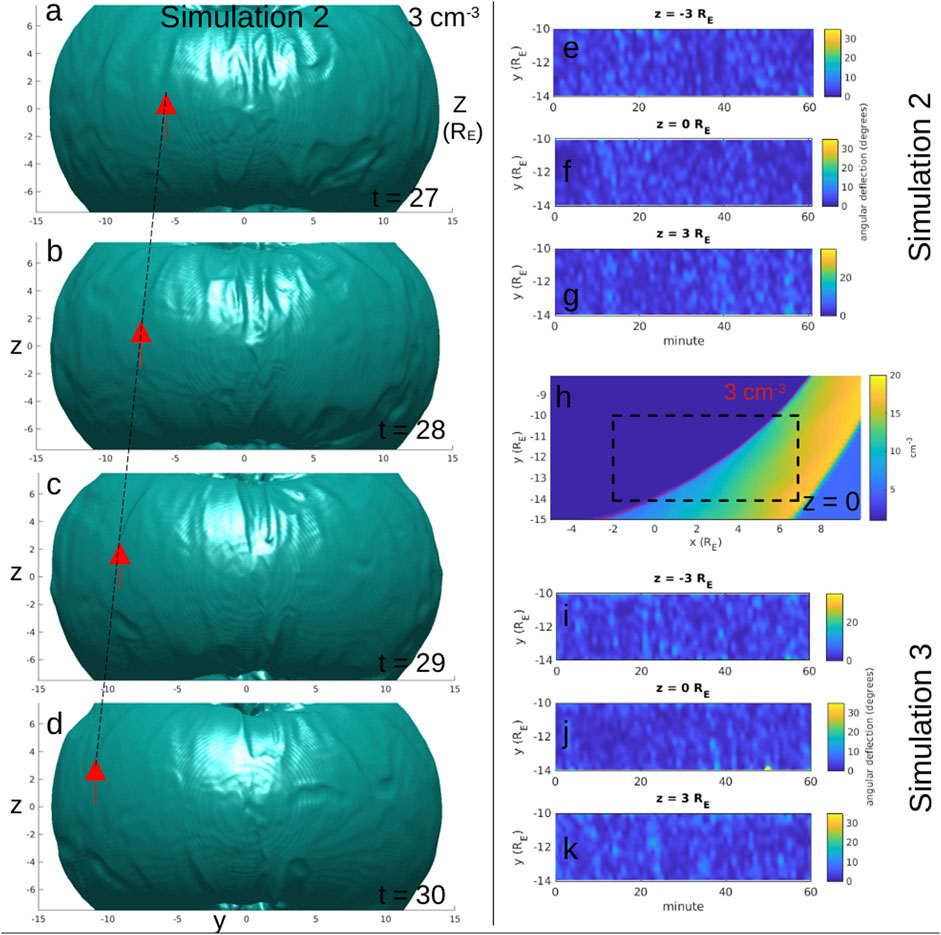
FIGURE 8. (A–D) Three-dimensional contours of plasma density (enclosing ρ > 3 cm−3) in simulation 2 with 1-min time separations. The value 3 cm−3 is chosen to represent the magnetopause boundary and the view is from the y-z plane. Red arrows with black dashed line show a surface wave traveling toward the dawn flank. (E–K) Compares the presence of surface waves on the magnetopause in simulation 2 versus simulation 3. (H) Highlights a portion of magnetopause boundary inside the black dashed box (colormap shows the plasma density and red contour is the value 3 cm−3 at z = 0 in simulation 2). The unperturbed boundary normal vectors are determined for each simulation by averaging the red contour over all time steps and panels (E–G) and (I–K) plot the instantaneous angular deflections from the unperturbed state along the y-coordinate range −14 to −10 RE. The z-cut for each time series is labeled in the corresponding title.
Figure 6 demonstrates that flux ropes spontaneously formed on the magnetopause boundary (in simulation 2) have a finite width in local time, which leads to a discontinuous structure of the x-line. Figure 6A is a three-dimensional representation of the simulation with closed magnetosphere field lines colored blue, magnetopause boundary colored red, and a magnetopause flux rope generated by day-side reconnection in black. The core of this magnetic flux rope is composed of flux mapping to the inner boundary of the simulation on both ends, while the whole 1–2 RE scale (diameter of the flux rope) structure is mostly made of flux with 1 end mapping to the inner boundary (not drawn in the 3D representation). Figures 6B–J compare magnetic flux rope connectivities at different y-cuts of the simulation. Each panel (b-j) shows a magnetic connectivity map in the y = −5 RE (left), y = 0 RE (middle), or y = 5 RE (right) plane, with each row at a different time step (labeled on the right of the figure). Purple represents magnetic flux that is closed (mapping to the inner boundary of the simulation) at both ends, orange closed at 1 end only, and blue open at both ends. Figure 6B shows a cut through the flux rope drawn in Figure 6A; Figures 6E, H show this flux rope moving towards the northern cusp (at about 1 RE/min). At the corresponding time steps, this same flux rope can not be identified at y = 0 (Figures 6C,F,I) or y = 5 RE (Figures 6D,G,J). This is because flux rope formation is spontaneous in these idealized simulations, and the entire DXL does not form a flux rope at the same time. Comparison of the simulation 1 and 2 movies in the Supplementary Material shows that for purely southward IMF the flux ropes have smaller extent in local time for higher simulation resolution. In simulation 1 their width is at minimum about 3–4 RE while in simulation 2 it is at minimum 1–2 RE. This is not surprising since simulation 2 has twice the resolution of simulation 1 (in each coordinate dimension), although the diameters of the flux ropes are similar for both simulations. It remains an open question whether these trends continue for higher resolution.
To investigate the relative occurrence of flux ropes in simulations 2 and 4, three-dimensional contours of the thermal pressure are examined at a value of 1.25 nPa, which reveals the pressure enhancements associated with flux ropes on the magnetopause (Dorelli and Bhattacharjee, 2009; Sun et al., 2019). Figure 7A shows the pressure contour in simulation 2 at the same time step as Figure 6A. The closed flux core of the flux rope is perfectly encased by the red pressure contour. Figure 7B shows t = 32 min, which has multiple pressure enhancements on the magnetopause boundary. The three dimensional magnetic field lines traced through each of the pressure enhancements confirm that each one is associated with a magnetic flux rope. Note these do not all have a core of closed-flux, many are composed of only singly-open flux. An advantage of the idealized solar wind conditions is that a single value of the pressure is sufficient to identify flux ropes throughout the entire duration of the simulation. Therefore, to compare the rate of flux rope production across the three-dimensional day-side magnetopause in simulations 2 and 4, Figures 7C, D show all of the 1.25 nPa contours for 1 h of the simulation at 1 min output resolution. Clearly, simulation 4 generates fewer flux ropes than simulation 2, which is the reason the average x-line length calculated in Figure 5 was smaller in simulation 4 than simulation 2.
Observations have shown that flux transfer events occur about 45% of the time when the IMF has a southward component, with the highest rates for due southward IMF (Berchem and Russell, 1984), in agreement with our conclusion above. Hasegawa (2012) discussed the scenario of more than one X-line on the magnetopause during southward IMF, leading to large scale (1–2 RE) flux rope formation that was shown in simulations for the first time by Raeder (2006). When multiple flux ropes exist on the magnetopause at any one time, Winglee et al. (2008) described a three-dimensional “rippling” of the day-side magnetopause, similar to the time-dependent orientation of the three-dimensional x-line demonstrated here.
In addition to flux ropes, surface waves on the magnetopause boundary also lead to time-dynamics of the DXL orientation. These waves cause local deflections of the magnetopause normal direction, modifying the magnetic shear angle and therefore the structure of the global DXL. The presence of these waves is demonstrated in simulation 2 in Figures 8A–D in the same way as Michael et al. (2021), using a three-dimensional contour of the density as a proxy for the magnetopause boundary. The time separation is 1 min between panels and the contour is drawn at a value of 3 cm−3. The red arrow tracks a surface wave from t = 27 min when it is near x = −5 RE to t = 30 min when it is beyond y = −10 RE on the dawn flank. The dashed black line indicates it is moving at nearly constant velocity down-tail.
Figures 8E–K demonstrate that more surface wave activity is present on the magnetopause boundary in simulation 3 compared to simulation 2. For context, Figure 8H shows a cut of the plasma density at z = 0 RE in simulation 2. The red contour shows the value of 3 cm−3. The dashed black box outlines a subdomain where the red contour is calculated for each 1-min output of the simulation and then used to construct an average curve with y-range of −14 to −10 RE, representing an unperturbed magnetopause shape within the subdomain. At each time step the angular deflection of the instantaneous magnetopause shape from the unperturbed curve is plotted in Figures 8E–G for simulation 2. The rows from top to bottom show deflections at z = −3 RE, z = 0 RE, and z = 3 RE, respectively. The same procedure is applied to simulation 3 in Figures 8I–K. Surface waves are active on the flank regions in both simulations 2 and 3, and there is noticeably more activity in simulation 3. The presence of surface waves on the flank region affects the shape of the boundary and therefore the structure of the global day-side magnetopause x-line. This is why the average x-line length calculated in Figure 5 was larger in simulation 3 compared to simulation 2.
6 Discussion and conclusion
The GAMERA simulation results provide support that the MMS observations in Figure 1 during steady IMF can be attributed to the time-dependent structure of the DXL when southward magnetic fields abut the magnetopause. Although, Fuselier et al. (2019) concluded that the x-line was quasi-stationary after examining 2 magnetopause boundary crossings under southward IMF and having |By| > |Bz|. The FTE production rate in the simulations in this study is very high due to the strongly southward IMF orientations. Therefore, a full sensitivity study of the x-line dynamics during different solar wind and IMF orientations is warranted in the future. Phan et al. (2000) observed an x-line that was at least 3 RE long during persistent southward IMF and argued that it was likely much longer. The x-line lengths calculated in Figure 5 extend over the entire day-side in local time, but during strongly southward IMF the observed length would more likely correspond to an individual segment of the x-line due to the step-like discontinuities in the global DXL structure. For simulation 2 this is generally about
The MHD simulations in this study during steady strongly southward IMF show spontaneously formed flux ropes and surface waves on the magnetopause boundary are both present. Raeder (2006) demonstrated how flux ropes form on the magnetopause but also found FTEs only develop for large dipole tilt. However, more recent global MHD simulations have shown FTEs can still form without a dipole tilt (Dorelli and Bhattacharjee, 2009; Glocer et al., 2016), in agreement with the time-dynamics of the global-scale structures investigated in this study. Furthermore, a complete description of how surface waves and flux ropes are interacting will require higher resolution simulations and is left for future study. Indeed, the presence of surface waves and flux ropes on the magnetopause have been shown in previous simulations, but this study for the first time demonstrates their effect on the time evolution of the global DXL during steady solar wind driving. In addition, it should be noted that while the IMF is rarely steady for an entire hour, it is often steady for ∼10 min, longer than the time-scale of variations in Figure 5, which is sufficient to make apparent the time-dependent structure of the DXL in our simulations. This has implications for dispersion signatures observed by satellites in the cusp (Connor et al., 2015). The cross polar cap potential may also vary along with the x-line length, which will be explored in future studies. It is also the case that during strongly southward IMF the surface waves are least often observed (Kavosi and Raeder, 2015), which would imply that there are different sources of magnetopause structure depending on the IMF Bz, i.e., flux ropes for southward IMF and surface waves for other orientations.
Key conclusions about the global structure of the day-side magnetopause x-line in GAMERA MHD simulations.
• The x-line during southward IMF extends across the day-side magnetopause and is a discontinuous, time-dynamic structure, varying on a time scale of minutes during steady solar driving.
• The maximum magnetic shear model represents a time averaged state of the magnetic shear angle on the magnetopause surface.
• The x-line complexity during strongly southward IMF increases with higher solar wind velocity (due to surface waves) and a small component of By decreases the complexity (due to less flux rope generation).
Lastly, it should be noted that Glocer et al. (2016), for instance, described a method to identify magnetic separators which when applied to global magnetosphere simulations traces out the DXL, and other methods exist to search for reconnection in simulations. However, for strongly southward IMF scenarios, Figures 3E, F show that the x-line can be visualized with little effort, since the particular symmetry affords contours of vz that trace the x-line. In this study the fast flow reversal provides confirmation of active reconnection while Figures 3A–D are based on tracing a large number of field lines, similar to other topological studies of the magnetopause (e.g., Komar et al., 2013; Guo et al., 2020). These visualizations allow to compare with the maximum magnetic shear model and to calculate the time-dependent length as a measure of the complexity of the global DXL.
Data availability statement
The datasets presented in this study can be found in online repositories. The names of the repository/repositories and accession number(s) can be found below: doi:10.5281/zenodo.7675548.
Author contributions
BB performed the simulations and wrote the manuscript. L-JC provided funding and advised BB. KS, AS, and SM provided simulation expertise. KT provided the maximum magnetic shear model plots. DG, XM, and HK helped with preparing the manuscript. All authors contributed to the article and approved the submitted version.
Funding
Funding for this work is provided by the NASA MMS Mission and MMS Early Career Grant 80NSSC22K0949. The research at LASP is supported by NASA grants NNX14AF71G, 80NSSC20K0688 and 80NSSC19K0849. The research at JHU/APL was supported by the NASA DRIVE Science Center for Geospace Storms under grant 80NSSC20K0601 (Phase I) and cooperative agreement 80NSSC22M0163 (Phase II), as well as NASA grants 80NSSC19K0241, 80NSSC20K1833, 80NSSC19K0080, and 80NSSC19K0071.
Acknowledgments
We acknowledge use of NASA/GSFC’s Space Physics Data Facility’s OMNIWeb. The authors acknowledge the Texas Advanced Computing Center (TACC) at The University of Texas at Austin for providing HPC resources that have contributed to the research results reported within this paper http://www.tacc.utexas.edu.
Conflict of interest
The authors declare that the research was conducted in the absence of any commercial or financial relationships that could be construed as a potential conflict of interest.
Publisher’s note
All claims expressed in this article are solely those of the authors and do not necessarily represent those of their affiliated organizations, or those of the publisher, the editors and the reviewers. Any product that may be evaluated in this article, or claim that may be made by its manufacturer, is not guaranteed or endorsed by the publisher.
Supplementary material
The Supplementary Material for this article can be found online at: https://www.frontiersin.org/articles/10.3389/fspas.2023.1175697/full#supplementary-material
References
Arnold, H., Sorathia, K., Stephens, G., Sitnov, M., Merkin, V. G., and Birn, J. (2023). Data mining inspired localized resistivity in global mhd simulations of the magnetosphere. J. Geophys. Res. Space Phys.128, e2022JA030990. doi:10.1029/2022JA030990
Berchem, J., and Russell, C. T. (1984). Flux transfer events on the magnetopause: Spatial distribution and controlling factors. J. Geophys. Res. Space Phys.89, 6689–6703. doi:10.1029/JA089iA08p06689
Burch, J. L., Moore, T. E., Torbert, R. B., and Giles, B. L. (2016a). Magnetospheric multiscale overview and science objectives. Space Sci. Rev.199, 5–21. doi:10.1007/s11214-015-0164-9
Chen, L.-J., Ng, J., Omelchenko, Y., and Wang, S. (2021a). Magnetopause reconnection and indents induced by foreshock turbulence. Geophys. Res. Lett.48, e2021GL093029. doi:10.1029/2021GL093029
Connor, H. K., Raeder, J., Sibeck, D. G., and Trattner, K. J. (2015). Relation between cusp ion structures and dayside reconnection for four imf clock angles: Openggcm-ltpt results. J. Geophys. Res. Space Phys.120, 4890–4906. doi:10.1002/2015JA021156
Denton, R. E., Sonnerup, B. U. O., Russell, C. T., Hasegawa, H., Phan, T.-D., Strangeway, R. J., et al. (2018). Determining l-m-n current sheet coordinates at the magnetopause from magnetospheric multiscale data. J. Geophys. Res. Space Phys.123, 2274–2295. doi:10.1002/2017JA024619
Dorelli, J. C., and Bhattacharjee, A. (2009). On the generation and topology of flux transfer events. J. Geophys. Res. Space Phys.114. doi:10.1029/2008JA013410
Dorelli, J. C., Bhattacharjee, A., and Raeder, J. (2007). Separator reconnection at earth’s dayside magnetopause under generic northward interplanetary magnetic field conditions. J. Geophys. Res. Space Phys.112. doi:10.1029/2006JA011877
Dunlop, M. W., Zhang, Q.-H., Bogdanova, Y. V., Trattner, K. J., Pu, Z., Hasegawa, H., et al. (2011). Magnetopause reconnection across wide local time. Ann. Geophys.29, 1683–1697. doi:10.5194/angeo-29-1683-2011
Fedder, J. A., and Lyon, J. G. (1995). The Earth’s magnetosphere is 165 RE long: Self-consistent currents, convection, magnetospheric structure, and processes for northward interplanetary magnetic field. J. Geophys. Res.100, 3623–3635. doi:10.1029/94JA02633
Fuselier, S. A., Frey, H. U., Trattner, K. J., Mende, S. B., and Burch, J. L. (2002). Cusp aurora dependence on interplanetary magnetic fieldB<sub>z</sub>. J. Geophys. Res. Space Phys.107, 1111. SIA 6–1–SIA 6–10. doi:10.1029/2001JA900165
Fuselier, S. A., Trattner, K. J., Petrinec, S. M., Pritchard, K. R., Burch, J. L., Cassak, P. A., et al. (2019). Stationarity of the reconnection x-line at earth’s magnetopause for southward imf. J. Geophys. Res. Space Phys.124, 8524–8534. doi:10.1029/2019JA027143
Glocer, A., Dorelli, J., Toth, G., Komar, C. M., and Cassak, P. A. (2016). Separator reconnection at the magnetopause for predominantly northward and southward imf: Techniques and results. J. Geophys. Res. Space Phys.121, 140–156. doi:10.1002/2015JA021417
Gonzalez, W. D., and Mozer, F. S. (1974). A quantitative model for the potential resulting from reconnection with an arbitrary interplanetary magnetic field. J. Geophys. Res.79, 4186–4194. doi:10.1029/JA079i028p04186
Gosling, J. T., Thomsen, M. F., Bame, S. J., Elphic, R. C., and Russell, C. T. (1990). Plasma flow reversals at the dayside magnetopause and the origin of asymmetric polar cap convection. J. Geophys. Res. Space Phys.95, 8073–8084. doi:10.1029/JA095iA06p08073
Greene, J. M. (1988). Geometrical properties of three-dimensional reconnecting magnetic fields with nulls. J. Geophys. Res. Space Phys.93, 8583–8590. doi:10.1029/JA093iA08p08583
Guo, Z., Lin, Y., Wang, X., Vines, S. K., Lee, S. H., and Chen, Y. (2020). Magnetopause reconnection as influenced by the dipole tilt under southward imf conditions: Hybrid simulation and mms observation. J. Geophys. Res. Space Phys.125, e2020JA027795. doi:10.1029/2020JA027795
Hasegawa, H. (2012). Structure and dynamics of the magnetopause and its boundary layers. Monogr. Environ. Earth Planets1, 71–119. doi:10.5047/meep.2012.00102.0071
Jacobsen, K. S., Phan, T. D., Eastwood, J. P., Sibeck, D. G., Moen, J. I., Angelopoulos, V., et al. (2009). Themis observations of extreme magnetopause motion caused by a hot flow anomaly. J. Geophys. Res. Space Phys.114. doi:10.1029/2008JA013873
Kavosi, S., and Raeder, J. (2015). Ubiquity of Kelvin-Helmholtz waves at Earth’s magnetopause. Nat. Commun.6, 7019. doi:10.1038/ncomms8019
Komar, C. M., Cassak, P. A., Dorelli, J. C., Glocer, A., and Kuznetsova, M. M. (2013). Tracing magnetic separators and their dependence on imf clock angle in global magnetospheric simulations. J. Geophys. Res. Space Phys.118, 4998–5007. doi:10.1002/jgra.50479
Laitinen, T. V., Janhunen, P., Pulkkinen, T. I., Palmroth, M., and Koskinen, H. E. J. (2006). On the characterization of magnetic reconnection in global MHD simulations. Ann. Geophys.24, 3059–3069. doi:10.5194/angeo-24-3059-2006
Lau, Y.-T., and Finn, J. M. (1990). Three-dimensional Kinematic reconnection in the presence of field nulls and closed field lines. Astrophysical J.350, 672. doi:10.1086/168419
Lin, D., Sorathia, K., Wang, W., Merkin, V., Bao, S., Pham, K., et al. (2021). The role of diffuse electron precipitation in the formation of subauroral polarization streams. J. Geophys. Res. Space Phys.126, e2021JA029792. doi:10.1029/2021JA029792
Lyon, J. G., Fedder, J. A., and Mobarry, C. M. (2004). The Lyon-Fedder-Mobarry (LFM) global MHD magnetospheric simulation code. J. Atmos. Solar-Terrestrial Phys.66, 1333–1350. doi:10.1016/j.jastp.2004.03.020
Ma, X., Otto, A., and Delamere, P. A. (2014a). Interaction of magnetic reconnection and kelvin-helmholtz modes for large magnetic shear: 1. Kelvin-helmholtz trigger. J. Geophys. Res. Space Phys.119, 781–797. doi:10.1002/2013JA019224
Ma, X., Otto, A., and Delamere, P. A. (2014b). Interaction of magnetic reconnection and kelvin-helmholtz modes for large magnetic shear: 2. Reconnection trigger. J. Geophys. Res. Space Phys.119, 808–820. doi:10.1002/2013JA019225
Mejnertsen, L., Eastwood, J. P., and Chittenden, J. P. (2021). Control of magnetopause flux rope topology by non-local reconnection. Front. Astronomy Space Sci.8, 186. doi:10.3389/fspas.2021.758312
Merkin, V. G., Lyon, J. G., and Claudepierre, S. G. (2013). Kelvin-Helmholtz instability of the magnetospheric boundary in a three-dimensional global MHD simulation during northward IMF conditions. J. Geophys. Res. (Space Phys.118, 5478–5496. doi:10.1002/jgra.50520
Merkin, V. G., and Lyon, J. G. (2010). Effects of the low-latitude ionospheric boundary condition on the global magnetosphere. J. Geophys. Res. Space Phys.115. doi:10.1029/2010JA015461
Michael, A. T., Sorathia, K. A., Merkin, V. G., Nykyri, K., Burkholder, B., Ma, X., et al. (2021). Modeling kelvin-helmholtz instability at the high-latitude boundary layer in a global magnetosphere simulation. Geophys. Res. Lett.48, e2021GL094002. doi:10.1029/2021GL094002
Nykyri, K., and Otto, A. (2004). Influence of the hall term on kh instability and reconnection inside kh vortices. Ann. Geophys.22, 935–949. doi:10.5194/angeo-22-935-2004
Nykyri, K., and Otto, A. (2001). Plasma transport at the magnetospheric boundary due to reconnection in kelvin-helmholtz vortices. Geophys. Res. Lett.28, 3565–3568. doi:10.1029/2001GL013239
Ong, R., and Roderick, N. (1972). On the kelvin-helmholtz instability of the earth’s magnetopause. Planet. Space Sci.20, 1–10. doi:10.1016/0032-0633(72)90135-3
Ouellette, J. E., Rogers, B. N., Wiltberger, M., and Lyon, J. G. (2010). Magnetic reconnection at the dayside magnetopause in global lyon-fedder-mobarry simulations. J. Geophys. Res. Space Phys.115. doi:10.1029/2009JA014886
Peterson, W. K., Tung, Y.-K., Carlson, C. W., Clemmons, J. H., Collin, H. L., Ergun, R. E., et al. (1998). Simultaneous observations of solar wind plasma entry from fast and polar. Geophys. Res. Lett.25, 2081–2084. doi:10.1029/98GL00668
Pham, K. H., Zhang, B., Sorathia, K., Dang, T., Wang, W., Merkin, V., et al. (2022). Thermospheric density perturbations produced by traveling atmospheric disturbances during august 2005 storm. J. Geophys. Res. Space Phys.127, e2021JA030071. doi:10.1029/2021JA030071
Phan, T. D., Kistler, L. M., Klecker, B., Haerendel, G., Paschmann, G., Sonnerup, B. U. Ö., et al. (2000). Extended magnetic reconnection at the Earth’s magnetopause from detection of bi-directional jets. Nature404, 848–850. doi:10.1038/35009050
Phan, T. D., Paschmann, G., Gosling, J. T., Oieroset, M., Fujimoto, M., Drake, J. F., et al. (2013). The dependence of magnetic reconnection on plasma beta and magnetic shear: Evidence from magnetopause observations. Geophys. Res. Lett.40, 11–16. doi:10.1029/2012GL054528
Pinnock, M., and Rodger, A. S. (2000). On determining the noon polar cap boundary from SuperDARN HF radar backscatter characteristics. Ann. Geophys.18, 1523–1530. doi:10.1007/s00585-001-1523-2
Plaschke, F., Angelopoulos, V., and Glassmeier, K.-H. (2013). Magnetopause surface waves: Themis observations compared to mhd theory. J. Geophys. Res. Space Phys.118, 1483–1499. doi:10.1002/jgra.50147
Pollock, C., Moore, T., Jacques, A., Burch, J., Gliese, U., Saito, Y., et al. (2016). Fast plasma investigation for magnetospheric multiscale. Space Sci. Rev.199, 331–406. doi:10.1007/s11214-016-0245-4
Pu, Z. Y., and Kivelson, M. G. (1983). Kelvin-Helmholtz instability at the magnetopause: Solution for compressible plasmas. J. Geophys. Res.88, 841–852. doi:10.1029/JA088iA02p00841
Raeder, J. (2006). Flux transfer events: 1. Generation mechanism for strong southward IMF. Ann. Geophys.24, 381–392. doi:10.5194/angeo-24-381-2006
Russell, C. T., Anderson, B. J., Baumjohann, W., Bromund, K. R., Dearborn, D., Fischer, D., et al. (2016). The magnetospheric multiscale magnetometers. Space Sci. Rev.199, 189–256. doi:10.1007/s11214-014-0057-3
Russell, C. T., and Elphic, R. C. (1978). Initial ISEE magnetometer results: Magnetopause observations. Space Sci. Rev.22, 681–715. doi:10.1007/BF00212619
Scurry, L., Russell, C. T., and Gosling, J. T. (1994). A statistical study of accelerated flow events at the dayside magnetopause. J. Geophys. Res. Space Phys.99, 14815–14829. doi:10.1029/94JA00793
Sonnerup, B. U. Ö., Papamastorakis, I., Paschmann, G., and Lühr, H. (1987). Magnetopause properties from ampte/irm observations of the convection electric field: Method development. J. Geophys. Res. Space Phys.92, 12137–12159. doi:10.1029/JA092iA11p12137
Sonnerup, B. U. Ö., Paschmann, G., and Phan, T.-D. (1995). Fluid aspects of reconnection at the magnetopause: In situ observations (American geophysical union (AGU)). 167–180. doi:10.1029/GM090p0167
Sorathia, K. A., Merkin, V. G., Panov, E. V., Zhang, B., Lyon, J. G., Garretson, J., et al. (2020). Ballooning-interchange instability in the near-earth plasma sheet and auroral beads: Global magnetospheric modeling at the limit of the mhd approximation. Geophys. Res. Lett.47, e2020GL088227. doi:10.1029/2020GL088227
Sorathia, K. A., Merkin, V. G., Ukhorskiy, A. Y., Allen, R. C., Nykyri, K., and Wing, S. (2019). Solar wind ion entry into the magnetosphere during northward imf. J. Geophys. Res. Space Phys.124, 5461–5481. doi:10.1029/2019JA026728
Sorathia, K. A., Merkin, V. G., Ukhorskiy, A. Y., Mauk, B. H., and Sibeck, D. G. (2017). Energetic particle loss through the magnetopause: A combined global mhd and test-particle study. J. Geophys. Res. Space Phys.122, 9329–9343. doi:10.1002/2017JA024268
Souza, V. M., Gonzalez, W. D., Sibeck, D. G., Koga, D., Walsh, B. M., and Mendes, O. (2017). Comparative study of three reconnection x line models at the earth’s dayside magnetopause using in situ observations. J. Geophys. Res. Space Phys.122, 4228–4250. doi:10.1002/2016JA023790
Sun, T. R., Tang, B. B., Wang, C., Guo, X. C., and Wang, Y. (2019). Large-scale characteristics of flux transfer events on the dayside magnetopause. J. Geophys. Res. Space Phys.124, 2018JA026395–2434. doi:10.1029/2018JA026395
Swisdak, M., and Drake, J. F. (2007). Orientation of the reconnection x-line. Geophys. Res. Lett.34, L11106. doi:10.1029/2007GL029815
Trattner, K. J., Mulcock, J. S., Petrinec, S. M., and Fuselier, S. A. (2007). Probing the boundary between antiparallel and component reconnection during southward interplanetary magnetic field conditions. J. Geophys. Res. Space Phys.112. doi:10.1029/2007JA012270
Trattner, K. J., Petrinec, S. M., and Fuselier, S. A. (2021). The location of magnetic reconnection at earth’s magnetopause. Space Sci. Rev.217, 41. doi:10.1007/s11214-021-00817-8
Wiltberger, M., Merkin, V., Lyon, J. G., and Ohtani, S. (2015). High-resolution global magnetohydrodynamic simulation of bursty bulk flows. J. Geophys. Res. (Space Phys.120, 4555–4566. doi:10.1002/2015JA021080
Winglee, R. M., Harnett, E., Stickle, A., and Porter, J. (2008). Multiscale/multifluid simulations of flux ropes at the magnetopause within a global magnetospheric model. J. Geophys. Res. Space Phys.113. doi:10.1029/2007JA012653
Zhang, B., Lotko, W., Brambles, O., Wiltberger, M., and Lyon, J. (2015). Electron precipitation models in global magnetosphere simulations. J. Geophys. Res. (Space Phys.120, 1035–1056. doi:10.1002/2014JA020615
Keywords: magnetic reconnection, day-side magnetopause, global simulation, magnetohydro-dynamics, flux ropes, surface waves
Citation: Burkholder BL, Chen L-J, Sorathia K, Sciola A, Merkin S, Trattner KJ, Gershman D, Ma X and Connor H (2023) The complexity of the day-side X-line during southward interplanetary magnetic field. Front. Astron. Space Sci. 10:1175697. doi: 10.3389/fspas.2023.1175697
Received: 27 February 2023; Accepted: 04 July 2023;
Published: 18 July 2023.
Edited by:
Thomas Earle Moore, Third Rock Research, United StatesReviewed by:
Giovanni Lapenta, KU Leuven, BelgiumSteven Petrinec, Lockheed Martin Solar and Astrophysics Laboratory (LMSAL), United States
Copyright © 2023 Burkholder, Chen, Sorathia, Sciola, Merkin, Trattner, Gershman, Ma and Connor. This is an open-access article distributed under the terms of the Creative Commons Attribution License (CC BY). The use, distribution or reproduction in other forums is permitted, provided the original author(s) and the copyright owner(s) are credited and that the original publication in this journal is cited, in accordance with accepted academic practice. No use, distribution or reproduction is permitted which does not comply with these terms.
*Correspondence: Brandon L. Burkholder, YmxidXJraG9sZGVyQGFsYXNrYS5lZHU=