 Benjamin C. Martinez
 Xian Lu
- Department of Physics and Astronomy, Clemson University, Clemson, SC, United States
We quantify the short-term (<30 day) variability of column O/N2 measured by GOLD from January 2019 to August 2022 for various geomagnetic activity conditions. We find enhanced variabilities at high latitudes during active (Kp ≥ 3.0) times and weak but statistically significant variabilities at low latitudes. For active times, the largest absolute variability of O/N2 ratio is 0.14 and the largest relative variability is 20.6% at ∼60.0°N in Fall, which are about twice those of quiet times. The variability at higher latitudes can be larger than that of lower latitudes by a factor of 5–8. We further quantify contributions of magnetospheric forcing to O/N2 variability in the Ionosphere-Thermosphere region by correlating O/N2 perturbations with Dst. During geomagnetic active times, positive correlations as large as +0.66 and negative correlations as large as −0.65 are found at high and low latitudes, respectively, indicative of storm-induced O and N2 upwelling at high latitudes and down welling at low latitudes. During quiet times, correlations between O/N2 perturbations and Dst become insignificant at all latitudes, implying a more substantial contribution from below. O/N2 variabilities maximize in Fall and decrease towards Summer, while correlations maximize in Spring/Summer and decrease in Winter/Spring, which may be related to seasonal variations of geomagnetic activity and mean circulation.
1 Introduction
The Ionosphere-Thermosphere (IT) environment is strongly coupled to the magnetosphere above and the regions of the lower atmosphere below (Rishbeth et al., 2000). During active times, the short-term variability of the IT region is dominated by forcing from above in the form of enhanced magnetospheric forcing related to geomagnetic storms and substorms. During quiet times, the short-term variability of the IT region is modulated primarily by in-situ generated tides and/or upward-propagating waves originating from the lower atmosphere (Richmond, 1979; Rishbeth, 1997; Immel et al., 2006; Oberheide et al., 2011; Oberheide et al., 2013). Even during quiet times, however, solar geomagnetic activity can still have a significant impact on IT preconditioning (Cai et al., 2020), and it can take as long as 2 days for the IT to return to pre-storm conditions after a strong or moderate geomagnetic disturbance (Richmond et al., 2003; Lu et al., 2015; Yao et al., 2016). This makes the accurate characterization of the day-to-day variability difficult because it requires that we disentangle the effects of the different forcings in order to understand the relative contributions of each.
Strong agreement between the observed climatology of the IT region and the modeled climatology [from models like the Thermosphere-Ionosphere-Electrodynamics General Circulation Model (TIEGCM), its predecessor the Thermosphere General Circulation Model (TGCM), and the Whole Atmosphere Community Climate Model with thermosphere and ionosphere eXtension (WACCM-X)] has been demonstrated since as early as 1981 (Dickinson et al., 1981; Richmond et al., 1992; Fesen et al., 2002; Qian et al., 2014; Liu et al., 2018), but the day-to-day variations are comparatively difficult to model/study and therefore less understood (Zhou et al., 2020, Zhou et al., 2021; Andoh et al., 2022). Many details of the state of the IT system can be captured by parameters such as the ratio of atomic Oxygen (O) to molecular Nitrogen (N2) (O/N2). The seasonal O/N2 composition of the IT region depends, in particular, on global, vertical circulation in the ionosphere (Burns et al., 1995; Rishbeth et al., 2000; Qian et al., 2010; Luan et al., 2017; Li et al., 2022), the absorption of solar EUV during geomagnetic active periods, which changes the ratio via a combination of photodissociation and ionization processes (Kelley, 2009; Schmölter et al., 2020; Yu et al., 2020), and auroral heating-induced vertical winds which bring up atomic oxygen-poor air from the lower atmosphere (Hays et al., 1973).
The recently launched Global Observations of the Limb and Disk (GOLD) satellite provides full-disk ionospheric column O/N2 as a Level 2 data product from a geostationary orbit centered over the mouth of the Amazon River basin (Eastes et al., 2017). GOLD is the first satellite to observe the IT region from a fixed, geostationary orbit, which allows for the unambiguous separation of spatial and temporal IT variability and therefore makes possible unprecedented analysis of the day-to-day variability of O/N2. Recent studies have utilized GOLD O/N2 and temperature measurements to study seasonal variations of O/N2 as well as the response of O/N2 to both strong and weak geomagnetic activity (Cai et al., 2020; Laskar et al., 2021; Qian et al., 2022), but the seasonal, short-term response to varying geomagnetic activity levels has not yet been studied systematically across the full, presently available GOLD O/N2 dataset. Efforts to assimilate GOLD disk temperatures into whole atmosphere models have already led to significant improvements in model effective temperature root-mean square error (RMSE) (Laskar et al., 2021), and it should be possible to use GOLD O/N2 in a similar fashion to improve the abilities of models to capture day-to-day IT variability.
2 Data and methodology
2.1 GOLD data and data selection
GOLD measures the ratio of the vertical column density of O relative N2 defined at a standard reference N2 depth of 1017 cm−2. This reference depth is chosen to minimize uncertainty in O/N2 as a function of 135.6 nm/LBH and is equivalent to ∼4 nanobar, or ∼160 km (Correira et al., 2021). The O/N2 ratio is retrieved directly from dayside disk measurements of the OI-135.6 nm and N2-LBH band emission lines in the ∼134–164 nm wavelength range. We use version 3 of the O/N2 data product. The GOLD O/N2 data product is not optimized for auroral latitudes, so we limit our analysis to ±60° lat. The observations have longitudinal coverage ranging from 113.5°W to 19.5°E.
The O/N2 data from January 2019 to August 2022 and universal time (UTC) = ∼14:00–15:00 are used for the current study. This UTC time range is chosen because the full footprint of GOLD is illuminated at this time and because GOLD scanned at a cadence of one full disk every half hour from 2019–2021, and every hour in 2022. We omit several days in which the data are unreliable for instrumental reasons. We omit the data from the days surrounding a Gyrating Yaw Mechanism (GYM) actuation. GYM actuations, which lead to abrupt changes in 135.6 nm radiance and therefore make standard deviations unreliable, were applied twice in 2019 (4/26/2019 and 10/10/2019), twice in 2020 (3/20/2020 and 8/11/2020), and three times in 2021 (2/8/2021, 6/12/2021, and 8/27/2021) to mitigate the effects of detector burn-in. To quantify the uncertainties associated with each data point, we add the random, system, and model uncertainties reported for the column O/N2 data product in quadrature. We then omit all data points in which the uncertainties exceed 0.3.
For a particular UTC, there is a 2-D snapshot image of the O/N2 provided by GOLD for each individual day. In order to spatially suppress the noise, we take the average O/N2 ratio in a 10° × 10° (longitude × latitude) grid box and attribute this value to the center grid, and we collect all the data from January 2019 to August 2022 to each grid box. In order to have enough data points for calculating the standard deviation with significance, we omit all grid points where less than half of the days had reliable data. This results in the removal of much of the equatorial region, where uncertainties are generally higher because of flat-field correction errors (see the GOLD instrument documentation, available at https://gold.cs.ucf.edu/).
2.2 Calculation of short-term day-to-day variability
After binning the data for each grid box each day, we have obtained a time series with a temporal resolution of 1 day. We apply a 30-day high-pass filter to the time series at each longitude-latitude grid point to obtain the perturbations with periods shorter than 30 days, which are defined as O/N2 residuals hereinafter. After these perturbations are obtained, they are grouped together according to different seasons and their standard deviations (stds) are calculated. The seasonal and year-to-year variations are suppressed by the high-pass filter and therefore do not contribute to the std. The std is treated as a proxy for the day-to-day variability shorter than 30 days and longer than 2 days within a given season as a result of the temporal sampling (1 day) and filtering. Winter is defined as December, January, and February, Spring is defined as March, April, and May, Summer is defined as June, July, and August, and Fall/Autumn is defined as September, October, and November.
We consider all pre-screened data that fall into each season (∼270–360 points) first, then we divide the data into two activity classes categorized by Kp indices. We consider two separate activity thresholds based on Kp: days in which the maximum Kp ≥ 3.0 or 2.0 are considered to be active days, and days in which the maximum Kp < 3.0 or 2.0 were considered to be quiet days. To account for relatively long (∼24–48 h) IT recovery phases, we omit 1 day after each active day from the quiet day data. We use Kp to establish our quiet-time threshold to be consistent with, e.g., Cai et al. (2020). The stds are then calculated for these different groups of data (quiet, active, and all) and used to represent the variability under each condition. Finally, we calculate a relative std by dividing the absolute std by the quiet-time mean O/N2.
Geomagnetic conditions with the statistics of quiet and active days are summarized in Figure 1. In total, there are 440 active days (Kp ≥ 3.0) and 641 quiet days (Kp < 3.0). For the threshold of Kp = 2.0, there are 846 active days (Kp ≥ 2.0) and 220 quiet days (Kp < 2.0). Plotted Kp values are the daily maxima of 3-h Kp, and the reported Dst and F10.7 values are daily means. We choose daily maximum Kp as our quiet/active cutoff threshold in order to ensure that all days with any geomagnetic activity are considered active (using daily means could lead to misclassifications of days with short spikes of geomagnetic activity but low average Kp). We plot the solar F10.7 flux to show that our daily maximum Kp threshold is sufficient to account for periods of relatively high F10.7, and we show daily mean Dst because that value is used to track the O/N2 response to geomagnetic activity by correlating it with O/N2 residuals (see Section 3).
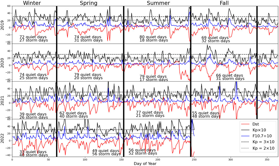
FIGURE 1. Solar and geomagnetic conditions for January 2019–August 2022. The solid black vertical lines divide the year into four seasons. Black, red, and blue lines show the daily maximum Kp, daily mean Dst (nT) and daily mean radio F10.7 (solar flux units). Dashed and dotted black lines show Kp = 3 and Kp = 2, respectively. The numbers in each box show the number of days with Kp ≥ 3.0 (storm days) and with Kp < 3.0 (quiet days). For viewing purposes, Kp index is multiplied by 10 and F10.7 is divided by 10.
3 Observations and results
Figure 2 shows the full-disk absolute stds of O/N2 perturbations as a proxy for the day-to-day variability with periods < 30 day in the IT region. Comparing different rows, variabilities are the strongest for Kp ≥ 3.0 (third row), with a maximum of 0.14 identified in Fall (Figure 2D3). Variabilities are the weakest during Kp < 2.0 (fourth row), with a maximum std of 0.07 also in Fall (Figure 2D4), which is about half of that in active time.
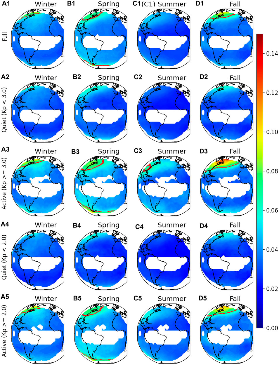
FIGURE 2. (A1–D1) Absolute stds of O/N2 ratios for the four seasons using all reliable data. (A2–D2), (A3–D3), (A4–D4) and (A5–D5) are the same except for the stds calculated using data with Kp < 3.0, Kp ≥ 3.0, Kp < 2.0 and Kp ≥ 2.0, respectively. Blank areas are regions where more than half of the daily O/N2 points had uncertainties exceeding 0.30. Red lines are the contours of 7.7%.
Figure 3 is the same as Figure 2 except for showing the relative stds of O/N2 perturbations. Relative stds are also the strongest when strong activities are considered (Kp ≥ 3.0) and decrease gradually towards moderate strong (Kp ≥ 2.0), moderate weak (Kp < 3.0) and the weakest (Kp < 2.0) conditions. We focus on the relative stds for the discussion of variabilities. For the Kp ≥ 3.0 case (third row of Figure 3), the averaged relative std is 4.9% across all seasons and grid points, and this value is 3.7% for Kp < 2.0, which gives a 28% difference between variabilities during most active and quiet times.
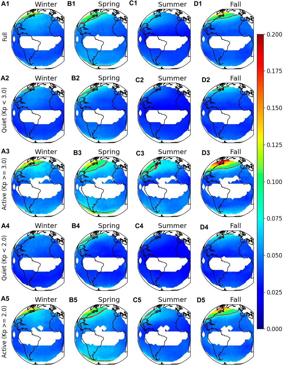
FIGURE 3. Same as Figure 2 except for relative stds. (A1–D1) are the relative stds of O/N2 ratios for the four seasons using all reliable data. (A2–D2), (A3–D3), (A4–D4), and (A5–D5) are the same except for the stds calculated using data with Kp < 3.0, Kp ≥ 3.0, Kp < 2.0, and Kp ≥ 2.0, respectively. Blank areas are regions where more than half of the daily O/N2 points had uncertainties exceeding 0.30. Red lines are the contours of 7.7%.
Variability is enhanced at high latitudes which may be related to auroral heating. For Kp ≥ 3.0 (third row), the highest variability observed is 20.6% at (70°W, 60.0°N) in Fall (Figure 2D3) and the weakest variability is 2.4% at (12°E, 6°N) in Summer which differs by a factor of 8–9 between high and low latitude variability for this activity category. During quiet conditions (Kp < 3.0, second row), the high latitude variability enhancement is weakened but still observed. The maximum variability is found to be ∼11.1% at a high latitude (70°W, 60°N) in Fall (Figure 3D2), which is about 4–5 times the minimum variability, that is, 2.4% at (8.0°E, 37°S) in Summer (Figure 3C2). The highest relative variability (20.6%) in active time is also about twice of that in quiet time (11.1%). The maximum and averaged variabilities for the various geomagnetic conditions and four seasons are plotted in Figures 6A, B.
In addition to the obvious latitudinal dependence, the magnitude of O/N2 variability and the extent of the high variability region at high northern latitudes also show a seasonal variation. The O/N2 maxima for the full dataset (Figures 3A1–D1) are 16%, 14%, 12% and 9% in Fall, Winter, Spring and Summer, which decrease from Fall to Summer. Maximum O/N2 variability also decreases from 21% to 11% from Fall to Summer for Kp ≥ 3.0. To quantify the extent of the high variability region which may be affected by aurora, we count all grid points where relative O/N2 stds exceed 7.7% (red contours in Figure 3) and convert that number to a percentage of the full GOLD field of view (fov). For each set of geomagnetic conditions, the extent of the region of influence is at maximum during Fall and Spring and at minimum during Winter and Summer. As an example, 5.0%, 13%, 2.5%, and 11% of the GOLD fov had relative O/N2 stds > 7.7% for Winter, Spring, Summer, and Fall, respectively considering the full dataset. The extents of the high variability region for different geomagnetic conditions and four seasons are illustrated in Figure 6C. It should be noted that 3–4 years of GOLD O/N2 data are used for this study: four Winters, Springs, and Summers and only three Falls. More data may help to better confirm the seasonal dependence.
From Figures 2, 3, variability increases with Kp index, which implies that magnetospheric forcing plays a role in the day-to-day variability of O/N2, especially at high latitudes. In order to better quantify this contribution, we calculate the correlation between the time series of O/N2 residuals and the Dst index. Figure 4 shows the correlation between these two parameters at (45°W, 59°N, a relatively high latitude region) during Summer and (2°W, 20°S, a relatively low latitude region) during Spring. The active-time data points (red in Figures 4A1, A2) are more tightly clustered than their quiet time (light blue) counterparts, and a linear fit shows a steep, positive (+0.66) correlation at (45°W, 59°N) and a steep negative (−0.65) correlation at (2°W, 20°S). In contrast, correlations are small when only quiet days are considered: +0.21 for (45°W, 59°N) and +0.07 for (2°W, 20°S). Magnitudes of the correlations decrease compared to active times when both quiet and active days are considered: they become +0.46 for (45°W, 59°N) and −0.38 for (2°W, 20°S). Figures 4B1, B2 show the time series of O/N2 residuals overplotted with Dst indices (both quiet and storm times are considered). The correlation at high latitudes and the anti-correlation at low latitudes are apparent.
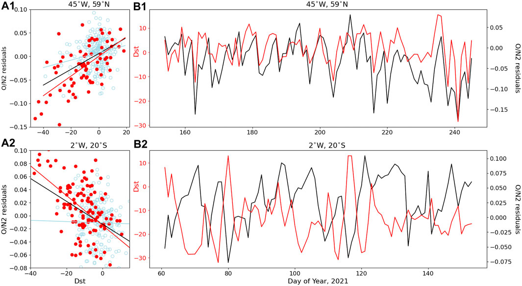
FIGURE 4. (A1,A2) O/N2 residuals versus Dst (scattered points) and their corresponding linear fits (straight lines) at (45°W, 59°N), and (2°W, 20°S). Light blue and red colors represent quiet and storm-times. The solid black line in each panel is fitted to all data points. (B1,B2) O/N2 residuals (black lines) and daily mean Dst (red lines) as a function of day of year at (45°W, 59°N), and (2°W, 20°N).
Shown in Figure 5 are the calculated correlation coefficients for each grid point in the GOLD fov for each season. Data gaps are present where correlations are determined to be insignificant based on a Student’s t-test and its associated p-value. We keep correlations where the p-value is less than 0.05, which means that the significance level of the correlation is greater than 95%. Figures 5A1–D1 show correlation maps where all reliable data for both quiet and storm conditions are considered. Red regions indicate positive correlations, and blue regions indicate negative correlations. Since Dst decreases in response to enhanced geomagnetic activity, a positive correlation means that the O/N2 ratio decreases as Dst decreases which corresponds to a storm-induced depletion in O/N2. A negative correlation means O/N2 ratio increases as Dst decreases, corresponding to a storm-induced enhancement in O/N2.
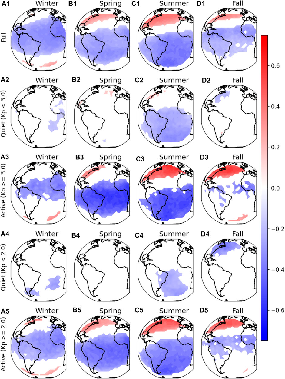
FIGURE 5. (A1–D1) Correlation maps between O/N2 residuals and Dst indices for the four seasons. Data gaps are present where the significance level is less than 95%. (A2–D2) and (A3–D3) are the same except only for quiet time (with Kp < 3.0) and active (Kp ≥ 3.0) times. (A4–D4) and (A5–D5) are the same except for quiet time with Kp < 2.0 and Kp ≥ 2.0 times.
By comparing different rows of Figure 5, which are grouped according to Kp, absolute correlations are the highest when large Kp values are considered (Kp ≥ 3.0, Figures 5A3–D3). Correlations as strong as +0.66 at (45°W, 59°N) and −0.65 at (2°W, 20°S) are observed during active time (Kp ≥ 3.0) in Summer (Figure 5C3). The highest correlations for Kp ≥ 2.0 are +0.55 at (45°W, 59°N) and −0.57 at (76°W, 55°S) in Summer (Figure 5C5). Maximum correlations for the full dataset (Figures 4A1–D1) are +0.47 at (72°W, 42°N) and −0.47 at (66°W, 54°S) during Summer (Figure 5C1). The maximum correlation and anti-correlation for the full dataset, and two active conditions are provided in Table 1.
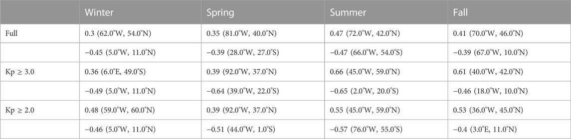
TABLE 1. The maximum correlation and largest anti-correlation for each season and activity class which includes active time data. The position of each correlation is given in parentheses.
There are very few significant correlations for quiet conditions (Kp < 3.0 and Kp < 2.0, Figures 5A2–D2, A4–D4) except for the quiet Summer. However, the region of significant correlation during Kp < 3.0 (Figure 5C2) shrinks significantly when only Kp < 2.0 is considered (Figure 5C4), which indicates that the threshold of Kp < 2.0 and the omission of 1 day after geomagnetic active days significantly reduces the contribution of magnetospheric forcing on IT variability. Cross-comparing Figures 2, 5, even though correlations are robust at both high and low latitudes during active times, variabilities are much larger at high latitudes, implying a more direct influence locally from aurora.
Similar to the variability, the extent of the positive correlation region and the maximum correlation show apparent seasonal dependencies. The extent of the positive correlation region is smallest during Winter (8.3% of the GOLD fov) and largest during Summer (27% of the GOLD fov) for the full dataset (Figure 6D). Similar trends exist for Kp ≥ 3.0 and Kp ≥ 2.0 of the positive correlation regions, and for maximum correlation values (Figure 6E). For example, when all data points are considered, the maximum positive correlations are 0.30, 0.35, 0.41, and 0.47 for Winter, Spring, Fall, and Summer respectively. The absolute values of largest anti-correlations for the three geomagnetic conditions (all data, Kp ≥ 3.0 and Kp ≥ 2.0) and four seasons are plotted in Figure 6F.
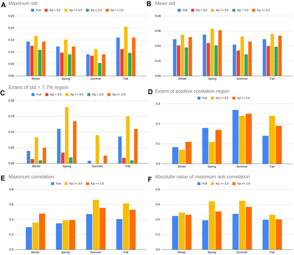
FIGURE 6. (A) Maximum and (B) mean standard deviation over the full disk for each season and each activity class. (C) Extent of the high variability region (relative stds ≥ 7.7%) as a percentage of the GOLD fov for each season and activity class. (D) Extent of the positive correlation region as a percentage of the GOLD fov. (E) Maximum positive correlation and (F) absolute value of maximum anti-correlation for each season and activity class.
4 Discussion and summary
The dependence of variability and correlation on Kp index, and the statistically significant correlation with Dst index indicate that the day-to-day O/N2 variabilities are strongly coupled to storm activities. Both auroral particle precipitation and Joule heating are enhanced during active times, with the auroral oval itself expanding and contracting with the activity level in a similar manner to the expansion and contraction of the high variability region (Figures 2, 3) and positive correlation region (Figure 5) observed at high latitudes. The fact that the high latitude enhancement in O/N2 variability is present (albeit weakened) during quiet times indicates that forcing from above can still dominate at high latitudes, regardless of geomagnetic activity levels.
The correlation maps shown in Figure 5 reflect the storm-induced, global, thermospheric circulation patterns which influence the distribution of O and N2. Joule heating causes the upwelling of N2-rich air and O-depleted air from the lower atmosphere, which is then distributed over high and mid latitudes by neutral winds (Strickland et al., 2004; Zhang et al., 2004; Zhang et al., 2015). The high latitude, positive correlation regions in Figure 5 are indicative of this upwelling. The corresponding negative correlations at low latitudes can be explained by the storm induced change in global circulation which drives low latitude downwelling (Fuller-Rowell et al., 2002). The low latitude response required to maintain continuity of mass flow is both delayed and weakened relative to the high latitude response (Forbes, 2007), which explains the smaller variabilities at low latitudes seen in Figures 2, 3. Based on this interpretation, the correlation map for the storm-time matches very closely the accepted circulation patterns for O and N2.
Luan et al. (2017) used data from the Global Ultraviolet Imager (GUVI) on board the TIMED (Thermosphere, Ionosphere, and Mesosphere, Energetics and Dynamics) satellite to obtain global maps of O/N2. The group reported larger values of O/N2 at high latitudes, which increased with increasing F10.7. They also reported significant longitudinal variations in O/N2 at a particular LT. These results compliment our own work, which instead focuses on the day-to-day variability of O/N2. Similar to the high latitude enhancement in mean O/N2 reported by Luan et al. (2017), we report high latitude enhancements in the day-to-day variability of O/N2 (Figures 2, 3). Luan et al. (2017) attributed the enhancement in mean O/N2 to auroral heating, which agrees with our own conclusions about auroral heating as the source of enhanced variability in O/N2.
Luan et al. (2017) also made use of TIE-GCM to further study the contribution of Joule heating to the observed O/N2 latitude-longitudinal patterns. This study showed that stronger auroral precipitation causes a decrease in O/N2 at high latitudes, which is consistent with the positive correlations between O/N2 and Dst that we report at high latitudes (Figure 5). Our work demonstrates that geomagnetic activity not only changes the absolute values of O/N2, it also contributes to the absolute and relative short-term temporal variability of O/N2. This implies that O/N2 changes more dramatically during storms and substorms.
The seasonal dependence of O/N2 variability and O/N2 residuals/Dst correlations may be partly explained by the seasonal dependence of auroral activity (Newell et al., 2010; Bower et al., 2022). O/N2 variabilities are strongest during Fall and Winter and weakest during Summer, which is consistent with observations of stronger auroral hemispheric power (HP) during Winter months (Zheng et al., 2013). Although auroral activity is at a minimum during Summer months, geomagnetic active-time upper thermospheric winds are at a maximum during these months (Dhadly and Conde, 2017), which may cause N2 rich and O poor air that has been brought up by upwelling to spread to lower latitudes. This may have the effect of increasing the auroral region of influence during Summer and enhancing the correlation, which is reflected in Figure 5.
In summary, the day-to-day (2–30 day) variability of GOLD O/N2 column density has been quantified and its correlation with Dst has been evaluated for various geomagnetic conditions and seasons for the first time. The main findings include:
1. Variability is significantly enhanced at high latitudes and during active (Kp ≥ 3.0) times, during which the largest absolute and relative variabilities of O/N2 ratio are found to be 0.14% and 21%, respectively, at ∼60.0°N in Fall. Variabilities are the weakest during Summer. Small but statistically significant variabilities are also observed at low latitudes and during quiet (Kp < 3.0) times. The maximum variability at high latitude during quiet times can decrease to half of the that during active times. The variability at low latitudes is smaller than that at high latitudes by a factor of 5–8 in general.
2. The active-time (Kp > 3.0) O/N2 residuals show the strongest positive correlation with Dst index at high latitude [+0.66 at (45°W, 59°N)] and strongest negative positive correlation at low latitude [−0.65 at (2°W, 20°S)] in Summer. Quiet-time correlation with Dst index is not statistically significant.
3. Correlations between Dst and O/N2 residuals become insignificant across the GOLD fov when only quiet (Kp < 2.0) days are considered, which implies a more substantial contribution from forcing from below to the observed variability during quiet conditions.
4. O/N2 variability and the correlation between Dst and O/N2 residuals have apparent seasonal dependencies. O/N2 variability is at a maximum during Fall and at minimum during Summer, whereas correlations are strongest during Summer and weakest during Winter.
This work has provided baseline/references for numerical models to capture the short-term variability of an important parameter (O/N2) of the IT system. To further diagnose the contributions from each source and find quantitative explanations for the ways that chemistry, dynamics, and electrodynamics contribute to the observed variability, for instance geomagnetic origin versus lower-atmosphere forcing, we will involve model sensitivity runs in a future work.
Data availability statement
Publicly available datasets were analyzed in this study. This data can be found here: https://gold.cs.ucf.edu/data/search/.
Author contributions
BM and XL contributed to conceptualization, methodology, and writing. BM performed the analysis. XL contributed to funding acquisition, investigation, supervision, and review editing. All authors have read and agreed to the published version of the manuscript.
Funding
This work is supported by NASA 80NSSC22K0018, NNX17AG10G, 80NSSC22K1010, 80NSSCK19K0810, and NSF AGS-2149695 and CAREER-1753214, and AGS-2012994.
Acknowledgments
We are grateful for discussions with Jens Oberheide and Haonan Wu at Clemson University, Jintai Li at University of Alaska, Fairbanks, Richard Eastes and Quan Gan at LASP, University of Colorado Boulder, and Nick Pedatella at the High Altitude Observatory, NCAR.
Conflict of interest
The authors declare that the research was conducted in the absence of any commercial or financial relationships that could be construed as a potential conflict of interest.
Publisher’s note
All claims expressed in this article are solely those of the authors and do not necessarily represent those of their affiliated organizations, or those of the publisher, the editors and the reviewers. Any product that may be evaluated in this article, or claim that may be made by its manufacturer, is not guaranteed or endorsed by the publisher.
References
Andoh, S., Saito, A., and Shinagawa, H. (2022). Numerical simulations on day-to-day variations of low-latitude Es layers at Arecibo. Geophys. Res. Lett. 49, e2021GL097473. doi:10.1029/2021GL097473
Bower, G. E., Milan, S. E., Paxton, L. J., and Anderson, B. J. (2022). Occurrence statistics of horse collar aurora. J. Geophys. Res. Space Phys. 127, e2022JA030385. doi:10.1029/2022JA030385
Burns, A. G., Killeen, T. L., Carignan, G. R., and Roble, R. G. (1995). Large enhancements in the O/N2 ratio in the evening sector of the winter hemisphere during geomagnetic storms. J. Geophys. Res. 100 (A8), 14661–14671. doi:10.1029/94JA03235
Cai, X., Burns, A. G., Wang, W., Coster, A., Qian, L., Liu, J., et al. (2020). Comparison of GOLD nighttime measurements with total electron content: Preliminary results. J. Geophys. Res. Space Phys. 125, e2019JA027767. doi:10.1029/2019JA027767
Correira, J., Evans, J. S., Lumpe, J. D., Krywonos, A., Daniell, R., Veibell, V., et al. (2021). Thermospheric composition and solar EUV flux from the global-scale observations of the Limb and disk (GOLD) mission. J. Geophys. Res. Space Phys. 126, e2021JA029517. doi:10.1029/2021JA029517
Dhadly, M., and Conde, M. (2017). Trajectories of thermospheric air parcels flowing over Alaska, reconstructed from ground-based wind measurements. J. Geophys. Res. Space Phys. 122, 6635–6651. doi:10.1002/2017JA024095
Dickinson, R. E., Ridley, E. C., and Roble, R. G. (1981). A three-dimensional general circulation model of the thermosphere. J. Geophys. Res. 86 (A3), 1499–1512. doi:10.1029/JA086iA03p01499
Eastes, R. W., McClintock, W. E., Burns, A. G., Anderson, D. N., Andersson, L., Codrescu, M., et al. (2017). The global-scale observationsof the Limb and disk (GOLD) mission. Space Sci. Rev. 212 (1–2), 383–408. doi:10.1007/s11214-017-0392-2
Fesen, C. G., Hysell, D. L., Meriwether, J. M., Mendillo, M., Fejer, B. G., Roble, R. G., et al. (2002). Modeling the low-latitude thermosphere and ionosphere. J. Atmos. Sol. Terr. Phys. 64, 1337–1349. doi:10.1016/s1364-6826(02)00098-6
Forbes, J. M. (2007). Dynamics of the thermosphere. J. Meteorol. Soc. Jpn. 85B, 193–213. doi:10.2151/jmsj.85b.193
Fuller-Rowell, T. J., Millward, G. H., Richmond, A. D., and Codrescu, M. V. (2002). Storm-time changes in the upper atmosphere at low latitudes. J. Atmos. Solar-Terrestrial Phys. 64 (12–14), 1383–1391. doi:10.1016/s1364-6826(02)00101-3
Hays, P. B., Jones, R. A., and Rees, M. H. (1973). Auroral heating and the composition of the neutral atmosphere. Planet. Space Sci. 21 (4), 559–573. doi:10.1016/0032-0633(73)90070-6
Immel, T. J., Sagawa, E., England, S. L., Henderson, S. B., Hagan, M. E., Mende, S. B., et al. (2006). Control of equatorial ionospheric morphology by atmospheric tides. Geophys. Res. Lett. 33, L15108. doi:10.1029/2006GL026161
Kelley, M. C. (2009). The earth’s ionosphere: Plasma physics and electrodynamics, international geophysics series, 43. Academic Press.
Laskar, F. I., Eastes, R. W., Codrescu, M. V., Evans, J. S., Burns, A. G., Wang, W., et al. (2021). Response of GOLD retrieved thermospheric temperatures to geomagnetic activities of varying magnitudes. Geophys. Res. Lett. 48, e2021GL093905. doi:10.1029/2021GL093905
Li, Z., Luan, X., Lei, J., and Ren, D. (2022). A simulation study on the variation of thermospheric O/N2 with solar activity. J. Geophys. Res. Space Phys. 127, e2022JA030305. doi:10.1029/2022JA030305
Liu, H.-L., Bardeen, C. G., Foster, B. T., Lauritzen, P., Liu, J., Lu, G., et al. (2018). Development and validation of the whole atmosphere community climate model with thermosphere and ionosphere extension (WACCM-X 2.0). J. Adv. Model. Earth Syst. 10, 381–402. doi:10.1002/2017MS001232
Lu, G., Hagan, M. E., Häusler, K., Doornbos, E., Bruinsma, S., Anderson, B. J., et al. (2015). Global ionospheric and thermospheric response to the 5 April 2010 geomagnetic storm: An integrated data-model investigation. J. Geophys. Res. Space Phys. 119 (10), 375. doi:10.1002/2014JA020555
Luan, X., Wang, W., Burns, A., and Dou, X. (2017). Solar cycle variations of thermospheric O/N2 longitudinal pattern from TIMED/GUVI. J. Geophys. Res. Space Phys. 122, 2605–2618. doi:10.1002/2016JA023696
Newell, P. T., Sotirelis, T., and Wing, S. (2010). Seasonal variations in diffuse, monoenergetic, and broadband aurora. J. Geophys. Res. 115, A03216. doi:10.1029/2009JA014805
Oberheide, J., Forbes, J. M., Zhang, X., and Bruinsma, S. L. (2011). Climatology of upward propagating diurnal and semidiurnal tides in the thermosphere. J. Geophys. Res. 116, A11306. doi:10.1029/2011JA016784
Oberheide, J., Mlynczak, M. G., Mosso, C. N., Schroeder, B. M., Funke, B., and Maute, A. (2013). Impact of tropospheric tides on the nitric oxide 5.3 μm infrared cooling of the low-latitude thermosphere during solar minimum conditions. J. Geophys. Res. Space Phys. 118, 7283–7293. doi:10.1002/2013JA019278
Qian, L., Burns, A. G., Emery, B. A., Foster, B., Lu, G., Maute, A., et al. (2014). “The NCAR TIE-GCM,” in Modeling the ionosphere–thermosphere system Editors J. Huba, R. Schunk, and G. Khazanov doi:10.1002/9781118704417.ch7
Qian, L., Gan, Q., Wang, W., Cai, X., Eastes, R., and Yue, J. (2022). Seasonal variation of thermospheric composition observed by NASA GOLD. J. Geophys. Res. Space Phys. 127, e2022JA030496. doi:10.1029/2022JA030496
Qian, L., Solomon, S. C., and Mlynczak, M. G. (2010). Model simulation of thermospheric response to recurrent geomagnetic forcing. J. Geophys. Res. 115, A10301. doi:10.1029/2010JA015309
Richmond, A. D. (1979). Large-amplitude gravity wave energy production and dissipation in the thermosphere. J. Geophys. Res. 84 (5), 1880–1890. doi:10.1029/JA084iA05p01880
Richmond, A. D., Peymirat, C., and Roble, R. G. (2003). Long-lasting disturbances in the equatorial ionospheric electric field simulated with a coupled magnetosphere-ionosphere-thermosphere model. J. Geophys. Res. 108, 1118. doi:10.1029/2002ja009758
Richmond, A. D., Ridley, E. C., and Roble, R. G. (1992). A thermosphere/ionosphere general circulation model with coupled electrodynamics. Geophys. Res. Lett. 19 (6), 601–604. doi:10.1029/92GL00401
Rishbeth, H. (1997). Long-term changes in the ionosphere. Adv. Space Res. 20 (11), 2149–2155. doi:10.1016/S0273-1177(97)00607-8
Rishbeth, H., Müller-Wodarg, I. C. F., Zou, L., Fuller-Rowell, T. J., Millward, G. H., Moffett, R. J., et al. (2000). Annual and semiannual variations in the ionospheric F2-layer: II. Physical discussion. Phys. Discuss. Ann. Geophys. 18, 945–956. doi:10.1007/s00585-000-0945-6
Schmölter, E., Berdermann, J., Jakowski, N., and Jacobi, C. (2020). Spatial and seasonal effects on the delayed ionospheric response to solar EUV changes. Ann. Geophys. 38, 149–162. doi:10.5194/angeo-38-149-2020
Strickland, D. J., Meier, R. R., Walterscheid, R. L., Craven, J. D., Christensen, A. B., Paxton, L. J., et al. (2004). Quiet-time seasonal behavior of the thermosphere seen in the far ultraviolet dayglow. J. Geophys. Res. 109, A01302. doi:10.1029/2003JA010220
Yao, Y., Liu, L., Kong, J., and Zhai, C. (2016). Analysis of the global ionospheric disturbances of the March 2015 great storm. J. Geophys. Res. Space Phys. 121, 12,157–12,170. doi:10.1002/2016JA023352
Yu, T., Ye, H., Liu, H., Xia, C., Zuo, X., Yan, X., et al. (2020). Ionospheric F layer scintillation weakening as observed by COSMIC/FORMOSAT-3 during the major sudden stratospheric warming in january 2013. J. Geophys. Res. Space Phys. 125, e2019JA027721. doi:10.1029/2019JA027721
Zhang, B., Lotko, W., Brambles, O., Wiltberger, M., and Lyon, J. (2015). Electron precipitation models in global magnetosphere simulations. J. Geophys. Res. Space Phys. 120, 1035–1056. doi:10.1002/2014JA020615
Zhang, Y., Paxton, L. J., Morrison, D., Wolven, B., Kil, H., Meng, C.-I., et al. (2004). O/N2 changes during 1–4 october 2002 storms: IMAGE SI-13 and TIMED/GUVI observations. J. Geophys. Res. 109, A10308. doi:10.1029/2004JA010441
Zheng, L., Fu, S., Zong, Q., Parks, G., Wang, C., and Chen, X. (2013). Solar cycle dependence of the seasonal variation of auroral hemispheric power. Chin. Sci. Bull. 58 (4–5), 525–530. doi:10.1007/s11434-012-5378-6
Zhou, X., Liu, H., Lu, X., Zhang, R., Maute, A., Wu, H., et al. (2020). Quiet-time day-to-day variability of equatorial vertical E×B drift from atmosphere perturbations at dawn. J. Geophys. Res. Space Phys. 125. doi:10.1029/2020JA027824
Keywords: day-to-day variability, GOLD, geomagnetic activity, auroral heating, O/N2 ratio, general circulation
Citation: Martinez BC and Lu X (2023) Quantifying day-to-day variability of O/N2 and its correlation with geomagnetic activity using GOLD. Front. Astron. Space Sci. 10:1129279. doi: 10.3389/fspas.2023.1129279
Received: 21 December 2022; Accepted: 09 February 2023;
Published: 20 February 2023.
Edited by:
Christina Arras, GFZ German Research Centre for Geosciences, GermanyReviewed by:
Juha Vierinen, UiT The Arctic University of Norway, NorwayAndrés Calabia, University of Alcalá, Spain
Copyright © 2023 Martinez and Lu. This is an open-access article distributed under the terms of the Creative Commons Attribution License (CC BY). The use, distribution or reproduction in other forums is permitted, provided the original author(s) and the copyright owner(s) are credited and that the original publication in this journal is cited, in accordance with accepted academic practice. No use, distribution or reproduction is permitted which does not comply with these terms.
*Correspondence: Benjamin C. Martinez, YmVuOEBjbGVtc29uLmVkdQ==
†These authors have contributed equally to this work and share first authorship