Semi-analytical orbital model around an oblate body with an inclined eccentric perturber

The semi-analytical model (based on the averaging technique) for long-term orbital evolution has proven to be useful in both astrophysical and astrodynamical contexts. In this secular approximation, orbits exhibit rich evolutionary behaviors under the effects of various perturbations. For example, in the hierarchical three-body systems, the Lidov-Kozai mechanism based on the quadrupole-level third-body perturbation model can produce large-amplitude oscillations of the eccentricity and inclination. In recent years, the octupole order has been found to induce dramatically new features when the perturbing body’s orbit is eccentric, including extremely high eccentricities and orbit flips between prograde and retrograde. Motivated by the striking effects of the octupole-order terms, we intend to derive a more general dynamical model by incorporating J₂ of the central body and the inclined eccentric third-body perturbation to the hexadecapole order with its non-spherical gravity also included. This issue can be relevant for astrophysical and astrodynamical systems such as planets in stellar binaries, irregular satellites in planetary systems, and artificial probes about binary asteroid systems. Applications to the binary asteroid system 4951 Iwamoto and a fictitious exoplanetary system are illustrated as examples to validate our secular model. From these numerical results, we show the high accuracy of our secular model. Also, we show the important role of these high-order terms and the effects of the third-body’s inclination and eccentricity. Besides, we have found several different secular effects that could drive large eccentricities.

1 Introduction

The secular perturbation theory was initially motivated by studying planetary and planetary satellite motions in the Solar system. The launch of artificial satellites in the 1960s, which brought new challenges and requirements, has sparked modern analyses of this problem. In complex perturbed environments, the semi-analytical model based on the averaging approach is widely employed as the standard technique in studying secular evolution, providing analytical insights into these perturbing effects, which is quite helpful for mission design. For example, orbital stability analysis (Scheeres et al., 2001; Lara and Juan, 2005; Fu and Wang, 2021), frozen orbit solutions (Delsate et al., 2010; Ulivieri et al., 2013; Condoleo et al., 2016; Circi et al., 2017), and orbits with specific evolution performances (Kamel and Tibbitts, 1973; Liu et al., 2010) have been extensively studied, and relevant results have been applied to a wide range of space missions, as well as lifetime reduction of space debris (Wang and Gurfil, 2016; Wang et al., 2020).

The motion of the hierarchical three-body system, in which the inner two bodies are orbited by an outer body in a wider orbit, is one of the most common problems in astrophysical and astrodynamical contexts. In astrodynamical settings, one of the inner bodies (generally, the spacecraft) can be considered massless, and its motion is dominated by the gravity of the central body and perturbed by the outer body (i.e., the third body or the perturbing body). Considering a highly hierarchical three-body system, the quadrupole level of approximation (also known as the Hill approximation, truncated to the second order of the semimajor axis ratio) is generally retained. In this approximation, based on the framework of the circular restricted-three body problem, both Lidov (1963); Kozai (1962) found that the system is axisymmetric after the double averaging over the inner and outer orbits, leading to the conservation of the z-component of the angular momentum of the inner orbit and, thereby, the integrability of this system. In particular, when the orbit inclination is above the critical inclination (∼$39.2°$), the eccentricity and inclination undergo long-periodic, large-amplitude oscillations. In the following decades, many studies have been devoted to this problem. Allan and Cook (1963) studied the orbital plane precession of circular orbits. The secular effect of the lunisolar perturbation on high-altitude earth satellites was analyzed (Broucke, 2003; De Moraes et al., 2008). The analytical solutions expressed in terms of Jacobi elliptic functions (Šidlichovskyý, 1983; Kinoshita and Nakai, 1991; Kinoshita and Nakai, 1999; Kinoshita and Nakai, 2007) or only simple trigonometric and hyperbolic functions (Lubow, 2021) were derived. By using the vectorial approach, Lara et al. (2020) developed the formulas for the expansion of the third-body disturbing function up to an arbitrary order, as well as long-term equations of motion by single averaging over the inner orbit.

We note that there are other two subcases in which the system exhibits more complex evolutionary behaviors but is still integrable based on a similar mechanism as the Lidov-Kozai ones (i.e., axisymmetry).

1) When the oblateness of the central body is further included but assuming a coplanar geometry (i.e., the perturbing body lies in the central body’s equator) (Kozai, 1969; Scheeres et al., 2001; Delsate et al., 2010; Fu and Wang, 2021). It has been found that the oblateness has changed the phase structures of the orbital dynamics by introducing new equilibrium points, and the critical inclination of the orbital stability changes as a function of the ratio between the perturbing forces of the oblateness and the third-body gravity (namely, the oblateness-related coefficient, $\kappa$, defined later) (Scheeres et al., 2001; Delsate et al., 2010).

2) The quadrupole-order approximation of the eccentric third-body perturbation (Lidov, 1963; Delsate et al., 2010; Naoz et al., 2013). That is, in the quadrupole-level model, even though the perturbing body is eccentric, the system is integrable. The eccentricity of the perturbing body only induces a small modification in the period of the eccentricity oscillation (De Moraes et al., 2008). However, this is an erroneous conclusion because the quadrupole level approximations have covered up the asymmetry of the system by the exclusion of the argument of perigee of the perturbing body’s orbit (which can be corrected by the octupole order). It has been found that the octupole order can cause a slow, cyclic modulation of the Lidov-Kozai cycles, resulting in orbit flips of the inner orbit (Katz et al., 2011; Lithwick and Naoz, 2011; Naoz, 2016), as well as chaotic motions (Li et al., 2014).

In fact, relaxing either one of the two assumptions (coplanarity or quadrupole-order approximation) will break the integrability of the system and thus lead to qualitatively different evolution behaviors. First, consider an inclined third-body perturbation. Different from the eccentric third-body perturbation problem, there is no special integral of motion in the quadrupole-level model compared to the higher-level models. Actually, only two integrals exist: the semi-major axis and the double-averaged perturbing potential (or the double-averaged Hamiltonian). There are only a few studies contributing to studying the secular evolution including the inclination of the perturbing body, and most of them were based on the quadrupole-order approximation (Yokoyama, 1999; Liu et al., 2012; Circi et al., 2017; Nie et al., 2019; Nie and Gurfil, 2021). Yokoyama (1999) pointed out that the high third-body inclination, with $J_2$ of the central body included, can produce strong chaotic motions and large eccentricities. Liu et al. (2012) and Nie et al. (2019) have developed a double-averaged model with the perturbing body in an eccentric and inclined orbit. However, although they assume an inclined eccentric perturbing body, the central body’s oblateness is not included, which, actually, can be related to the classical Lidov-Kozai mechanism via a coordinate transformation. Moreover, since the secular model is based on the quadrupole-order approximation, the critical features of the third-body eccentricity induced by the octupole order are not really included in their models. Then, consider a moderately hierarchical three-body system with an eccentric perturbing body. As stated above, when the perturbing boy’s orbit is eccentric, the quadrupole-order approximation is not enough to describe the secular dynamics and the octupole order is required. In the octupole-level model, the system can be very chaotic and extremely high eccentricities can be excited. In particular, the inner orbit can flip its orientation between prograde and retrograde periodically, accompanied by the eccentricity extremely approaching unity. This secular mechanism is also referred as the eccentric Lidov-Kozai effect (Naoz et al., 2011; Naoz, 2016). Beyond the octupole order, Naoz et al. (2013) point out that higher orders are expected to induce no more dramatic qualitative new features since the integrals of motion remain the same as the octupole order when moving to the higher orders. However, important modifications are possible. Carvalho et al. (2016) extended the perturbing potential to the hexadecapole and dotriocontupole orders and showed the importance of these high-order terms in changing the inversion times of the flip. Will (2017) presented the complete secular equations for both the inner and outer orbits to the hexadecapole order in classical orbit elements. He found that if the system has an equal-mass inner binary, the hexadecapole terms can alone generate orbit flips.

As a consequence, both the inclination and eccentricity of the perturbing body can break the integrability of the classical Lidov-Kozai mechanism. To the best of our knowledge, the two effects have been studied separately, but their joint effects have never been focused. Although several studies considered the eccentricity and inclination of the perturbing body simultaneously, they either focused on the quadrupole level of approximation, actually neglecting the critical effects of the third-body’s eccentricity, or they did not consider the central body’s oblateness, where the third-body’s inclination is actually a problem of coordinate selection.

On the other hand, in the astrophysical context, the discoveries of exoplanetary systems recently have promoted research into this problem (Tokovinin, 2014; Wang et al., 2015; Naoz, 2016; Moe and Kratter, 2021). Compared to the planets in the Solar system with nearly circular and coplanar configurations, the exoplanet systems are found to possess rich geometric architectures, such as eccentric and/or inclined planetary orbits as well as significant stellar oblateness and obliquity (Winn and Fabrycky, 2015). In recent years, dynamical behaviors involving highly eccentric orbits have been invoked to explain a wide range of astrophysical phenomena. For example, at the octupole order (i.e., third order of the semi-major axis ratio), the eccentric outer orbit can drive the inner orbit into extremely high eccentricities, and the sequent tidal dissipation near the pericenter rapidly circularizes that orbit, forming short-period even retrograde planets (Naoz et al., 2011; Naoz et al., 2013; Naoz, 2016). It has also been recently found that the oblateness of a rapidly rotating host star may be responsible for the large mutual inclinations of the exoplanetary systems (Li et al., 2020; Spalding and Millholland, 2020).

Therefore, we see that in a wide array of astrophysical and astrodynamical systems, the two effects can be simultaneously significant and strongly coupled. Concerning this, in this paper, we intend to develop a secular model including the perturbations of the central body’s oblateness and the gravity of an inclined eccentric perturbing body to the hexadecapole order (i.e., the fourth order of the semi-major axis ratio). In particular, the non-spherical gravity of the perturbing body is also incorporated to be applicable for asteroid systems. In order to simplify expressions, we formulate the equations of motion in terms of vectorial elements.

In what follows, we show the applications of our secular model to the binary asteroid system 4951 Iwamoto and a fictitious astrophysical system with assumed parameters to demonstrate its validity and to present some numerical results. Binary asteroid systems are pretty common in the solar asteroid population. About 16 per cent of near-Earth asteroids and main-belt asteroids with diameters below 10 km are binary systems. In recent years, many studies have been devoted to studying the orbital dynamics about these systems, including equilibrium and stability, as well as periodic orbits and invariant manifolds based on the restricted full three-body problem (Bellerose and Scheeres, 2008; Chappaz & Howell, 2015; Dell’Elce et al., 2017; Shi et al., 2019; Shi et al., 2020; Zhang et al., 2020; Li et al., 2021). Recently, Wang and Fu (2020) and Fu and Wang (2021) have extended the semi-analytical orbital theory to an orbiter of a binary asteroid system, assuming a coplanar and circular configuration, by retaining the third-body gravity to the hexadecapole order and including the non-spherical third-body gravity.

This paper is organized as follows. In Section 2, we present the exact Newtonian equations and the double-averaged equations to the hexadecapole order. The process of performing the double averaging, in the form of the vectorial elements, over the inner and outer orbits is elaborated. Next, we extend the hexadecapole-level model to include the non-spherical terms of the third-body gravity in Section 3. Then, we discuss a few applications in Section 4. We compare the different levels of approximation equations with the full equations to validate our semi-analytical model and to show some secular evolutionary behaviors. Finally, we conclude the paper in Section 5.

2 Double-averaged model to the hexadecapole order

In this Section, we derive the secular model of the hierarchical restricted three-body system beginning with the full Newtonian equations of motion. By using Legendre polynomials, the disturbing function of the perturbing body is truncated to the hexadecapole order. Then, the average over the inner and outer orbits is performed to filter out the high-frequency variations, arriving at equations that capture the secular orbital evolutions. The averaging results and the final equations are given in terms of the vectorial elements, where the mutual inclination between the central body’s equator and the perturbing body’s orbit is implied in the directions of these vectors.

2.1 Full equations of motion

The considered three-body system consists of a massless particle in a close orbit around the central body orbited by a perturbing body in a wider inclined and eccentric orbit (see Figure 1). In this part, the perturbing and the perturbed bodies are assumed to be point masses (the perturbing body in Figure 1 is depicted as an ellipsoid for later purposes), and the central body is an oblate spheroid. We choose the central body’s equatorial plane as the reference plane (the mutual orbit plane of the two massive bodies undergoes secular evolution when their non-spherical gravity is included and is therefore not suitable for the reference plane). The inertial reference frame $\left\{\mathit{x},\mathit{y},\mathit{z}\right\}$ is established with the origin located at the mass center of the central body and with the $x-y$ plane lying in the reference plane, the $x$ -axis initially along the nodal line of the perturbing body’s orbit, and the z-axis along the pole of the central body. For convenient, we represent the perturbing body’s orbital coordinate system as $\left\{{\widehat{\mathit{e}}}_{\mathrm{B}},{\widehat{\mathit{e}}}_{\perp \mathrm{B}},{\widehat{\mathit{h}}}_{\mathrm{B}}\right\}$ (the superscript denotes unit vector) where ${\mathit{e}}_{\mathrm{B}}$ is the orbit eccenrticity vector pointing to the periapse, ${\mathit{h}}_{\mathrm{B}}$ is the normalized orbit angular momentum vector, and ${\widehat{\mathit{e}}}_{\perp \mathrm{B}}$ complete the righ-hand coordinate system. If we ignore the evolution of the perturbing body’s orbit, this frame is also inertially fixed. Similarly, the particle’s orbital coordinate system can be denoted as $\left\{\widehat{\mathit{e}},{\widehat{\mathit{e}}}_{\perp },\widehat{\mathit{h}}\right\}$.

FIGURE 1

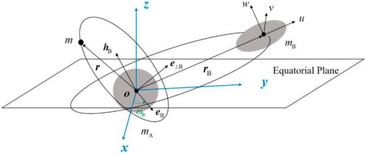
FIGURE 1. Geometry of the three-body system.

The perturbation effects of the perturbing body’s gravity on the particle can be stated in the potential form (called the disturbing function) as

$R_{\mathrm{P}\mathrm{B}}={\mu }_{\mathrm{B}}\left(\frac{1}{\left|\mathit{r}-{\mathit{r}}_{\mathrm{B}}\right|}-\frac{{\mathit{r}}_{\mathrm{B}}\cdot \mathit{r}}{r_{\mathrm{B}}^3}\right)(1)$

where ${\mu }_{\mathrm{B}}=G{m}_{\mathrm{B}}$ is the perturbing body’s gravitational parameter; ${\mathit{r}}_{\mathrm{B}}$ and $\mathit{r}$ are the position vectors of the perturbing body and the particle with respect to the central body’s mass center, respectively.

In hierarchical systems, the disturbing function can be expanded into an infinite series in the form of Legendre polynomials as

$R_{\mathrm{P}\mathrm{B}}=\frac{{\mu }_{\mathrm{B}}}{r_{\mathrm{B}}}{\displaystyle \sum }_{n=2}^{\infty }{\left(\frac{r}{r_{\mathrm{B}}}\right)}^n{P}_n\left(\widehat{\mathit{r}}\cdot {\widehat{\mathit{r}}}_{\mathrm{B}}\right)(2)$

where $P_n\left(x\right)$ are the Legendre polynomials about $x$. According to this formula, the disturbing function can be approximated by truncating the expansion to an arbitrary order, among which the lowest-order approximation, i.e., the quadrupole order, is most widely used in previous studies. However, if the three-body system is not highly hierarchical, especially when considering an eccentric perturbing body, the next several higher orders may be surprisingly important. To this end, here, we truncate the expansion to the hexadecapole order as

$R_{\mathrm{P}\mathrm{B}}=-\frac{{\mu }_{\mathrm{B}}}{2r_{\mathrm{B}}}\{{\left(\frac{r}{r_{\mathrm{B}}}\right)}^2\left[3{\left({\widehat{\mathit{r}}}_{\mathrm{B}}\cdot \widehat{\mathit{r}}\right)}^2-1\right]+{\left(\frac{r}{r_{\mathrm{B}}}\right)}^3\left[5{\left({\widehat{\mathit{r}}}_{\mathrm{B}}\cdot \widehat{\mathit{r}}\right)}^3-3\left({\widehat{\mathit{r}}}_{\mathrm{B}}\cdot \widehat{\mathit{r}}\right)\right]+{\left(\frac{r}{r_{\mathrm{B}}}\right)}^4\left[35{\left({\widehat{\mathit{r}}}_{\mathrm{B}}\cdot \widehat{\mathit{r}}\right)}^4-30{\left({\widehat{\mathit{r}}}_{\mathrm{B}}\cdot \widehat{\mathit{r}}\right)}^2+3\right]\}(3)$

The disturbing function of the oblateness of the central body can be represented by the gravitational coefficient $J_2$ as

$R_{J_2}=\frac{{\mu }_{\mathrm{A}}{J}_2{r}_{\mathrm{E}}^2}{2r^3}\left[1-3{\left(\widehat{\mathit{r}}\cdot \mathit{z}\right)}^2\right](4)$

where ${\mu }_{\mathrm{A}}=G{m}_{\mathrm{A}}$ is the gravitational parameter of the central body and $r_{\mathrm{E}}$ is its mean radius.

Then, the full Newtonian equations of motion, including perturbations of the central body’s oblateness and the third-body gravity, written in the inertial reference frame, are given as

$\ddot{\mathit{r}}=-\frac{{\mu }_{\mathrm{A}}}{r^3}\mathit{r}+\frac{\partial R_{J_2}}{\partial \mathit{r}}+\frac{\partial R_{\mathrm{P}\mathrm{B}}}{\partial \mathit{r}}(5)$

where the disturbing functions $R_{\mathrm{P}\mathrm{B}}$ and $R_{J_2}$ are given in Eqs. 1 and 4. If we replace the $R_{\mathrm{P}\mathrm{B}}$ in Eq. 5 with that in Eq. 3, we can obtain the hexadecapole-order (non-averaged) equations.

2.2 Semi-analytical model

In order to reduce the degrees of the system and provide analytical insight into the perturbation effects, the averaging method is proposed to eliminate the short-period terms and derive the equations that capture the long-term evolution of the system. According to the Krylov–Bogoliubov–Mitropolski method of averaging (Bogoliubov and Mitropolsky 1961; Rosengren, 2014), the averaging of the disturbing function is defined as

$\overline{R}\left(\mathit{\alpha }\right)=\frac{1}{2\pi }\underset{0}{\overset{2\pi }{{\displaystyle \int }}}R\left(\mathit{\alpha },M\right)dM(6)$

where $\mathit{\alpha }$ denotes the orbital elements except the mean anomaly $M$, which is proportional to time.

The validity of the averaging requires that $\mathit{\alpha }$ is nearly constant in the integration process. Physically, it requires the perturbation forces to be sufficiently small so that it follows a Keplerian orbit within one orbital period. In addition, in the current system, there are two frequencies related to the inner and outer orbital motion respectively. Then, it also requires that the two frequencies are away from each other and there is no resonance between them (the averaged model is not applicable when mean motion resonance occurs). The mean motions of the inner and outer orbits are given as

$n=\sqrt{{\mu }_{\mathrm{A}}/a^3}(7)$

$N_{\mathrm{B}}=\sqrt{{\mu }_{\mathrm{A}\mathrm{B}}/a_{\mathrm{B}}^3}(8)$

where $a$ is the inner orbit semimajor axis; ${\mu }_{\mathrm{A}\mathrm{B}}=G\left(m_{\mathrm{A}}+m_{\mathrm{B}}\right)$; $a_{\mathrm{B}}$ is the perturbing body’s semimajor axis. In the previous studies treating highly hierarchical systems, the conditions of the averaging are rarely discussed in detail. However, considering a stronger perturbed system with moderate hierarchy, these will be no longer negligible. In dealing with secular dynamics of a orbiter of an binary asteroid system, Wang and Fu (2020) have investigated the specific conditions of the averaging for systems with combined effects of the central body’s oblateness and third-body gravity. They concluded that, approximately, the perturbing forces should not exceed 1 per cent of the dominated central body’s gravity, and $n/N_{\mathrm{B}}$ should be less than 0.4. Therefore, for a given three-body system possessing the geometry in Figure 1, one can easily determine the range of the orbital altitude that ensures the reliability of the averaging. In the following calculations, we assume the averaging is performed within the valid range of the orbital altitude.

By the averaging theory, the secular Lagrange planetary equations in terms of vector elements, taking the compact and symmetrical form, are given by

$\left\{\begin{array}{c}\dot{\mathit{h}}=\mathit{h}\times \frac{\partial {\overline{R}}^{\prime }}{\partial \mathit{h}}+\mathit{e}\times \frac{\partial {\overline{R}}^{\prime }}{\partial \mathit{e}}\\ \dot{\mathit{e}}=\mathit{e}\times \frac{\partial {\overline{R}}^{\prime }}{\partial \mathit{h}}+\mathit{h}\times \frac{\partial {\overline{R}}^{\prime }}{\partial \mathit{e}}\end{array}\right.(9)$

where ${\overline{R}}^{\prime }$ is the averaged disturbing function scaled by $\sqrt{{\mu }_{\mathrm{A}}a}$ (where $a$ is constant in the averaged dynamics); $\mathit{h}=\mathit{H}/\sqrt{{\mu }_{\mathrm{A}}a}$ is the scaled orbit angular momentum; $\mathit{e}$ is the eccentricity vector. $\mathit{h}$ and $\mathit{e}$ in Eq. 9 denote mean elements (we drop the over bar for simplicity).

In the hierarchical three-body systems, as stated above, there are two timescales associated with the orbital motion $n$ and $N_{\mathrm{B}}$ respectively. Under certain conditions, averaging over the two timescales is feasible. We perform the first averaging over the mean anomaly of the inner orbit. The quadrupole order in Eq. 3 is averaged as

${\overline{R}}_{\mathrm{Q}\mathrm{u}\mathrm{a}}=-\frac{{\mu }_B}{2r_{\mathrm{B}}^3}\left[3{\widehat{\mathit{r}}}_{\mathrm{B}}\cdot \overline{\left(\mathit{r}\mathit{r}\right)}\cdot {\widehat{\mathit{r}}}_{\mathrm{B}}-\overline{r^2}\right](10)$

where the product of arbitrary two vectors $\mathit{a}\mathit{b}$ is called a dyad and, in the language of the matrix algebra, is equivalent to $\left[\mathit{a}\right]{\left[\mathit{b}\right]}^T$. The related terms are averaged as (Rosengren and Scheeres, 2013)

$\overline{r^2}=a^2\left(1+\frac{3}{2}{e}^2\right)(11)$

$\overline{\mathit{r}\mathit{r}}=\frac{1}{2}{a}^2\left[\left(1+4e^2\right)\widehat{\mathit{e}}\widehat{\mathit{e}}+\left(1-e^2\right){\widehat{\mathit{e}}}_{\perp }{\widehat{\mathit{e}}}_{\perp }\right](12)$

Substituting Eqs. 11–12 into Eq. 10, disregarding the irrelevant constant terms and scaling to $\sqrt{{\mu }_{\mathrm{A}}a}$, we have

${\overline{R}}_{\mathrm{Q}\mathrm{u}\mathrm{a}}^{\prime }=\frac{3{\mu }_B}{4n{r}_{\mathrm{B}}^3}\left[5{\left({\widehat{\mathit{r}}}_{\mathrm{B}}\cdot \mathit{e}\right)}^2-{\left({\widehat{\mathit{r}}}_{\mathrm{B}}\cdot \mathit{h}\right)}^2-2e^2\right](13)$

by virtue of the dyadic identity $\widehat{\mathit{e}}\widehat{\mathit{e}}+{\widehat{\mathit{e}}}_{\perp }{\widehat{\mathit{e}}}_{\perp }=I-\widehat{\mathit{h}}\widehat{\mathit{h}}$ in which $I$ denotes the identity matrix.

Averaging of the octupole-order terms in Eq. 3 requires (Rosengren, 2014)

$\overline{\mathit{r}}=-\frac{3}{2}a\mathit{e}(14)$

$\overline{r^2\mathit{r}}=-\frac{5}{8}{a}^3\left(4+3e^2\right)\mathit{e}(15)$

$\overline{\mathit{r}\mathit{r}\mathit{r}}=-\frac{5}{8}{a}^{3}e\left\{\left(3+4e^2\right)\widehat{\mathit{e}}\widehat{\mathit{e}}\widehat{\mathit{e}}+\left(1-e^2\right)\left[{\widehat{\mathit{e}}}_{\perp }{\widehat{\mathit{e}}}_{\perp }\widehat{\mathit{e}}+\widehat{\mathit{e}}{\widehat{\mathit{e}}}_{\perp }{\widehat{\mathit{e}}}_{\perp }+{\widehat{\mathit{e}}}_{\perp }\widehat{\mathit{e}}{\widehat{\mathit{e}}}_{\perp }\right]\right\}(16)$

where the product of three vectors $\mathit{a}\mathit{b}\mathit{c}$ is called a triad. To illustrate how it is calculated with other vectors, considering the averaging of ${\left({\widehat{\mathit{r}}}_{\mathrm{B}}\cdot \mathit{r}\right)}^3$ and by Eq. 16, we have

$\overline{{\left({\widehat{\mathit{r}}}_{\mathrm{B}}\cdot \mathit{r}\right)}^3}=-\frac{5}{8}{a}^3\left\{7{\left({\widehat{\mathit{r}}}_{\mathrm{B}}\cdot \mathit{e}\right)}^3+3\left({\widehat{\mathit{r}}}_{\mathrm{B}}\cdot \mathit{e}\right)\left[h^2-{\left({\widehat{\mathit{r}}}_{\mathrm{B}}\cdot \mathit{h}\right)}^2\right]\right\}(17)$

by dotting ${\widehat{\mathit{r}}}_{\mathrm{B}}$ with each of the vector elements in each triad on the right-hand side of Eq. 16. Through Eqs. 14–17, the octupole order is averaged as

${\overline{R}}_{\mathrm{O}\mathrm{c}\mathrm{t}}^{\prime }=-\frac{5{\mu }_{B}a}{16n{r}_{\mathrm{B}}^4}\left[35{\left({\widehat{\mathit{r}}}_{\mathrm{B}}\cdot \mathit{e}\right)}^3+3\left(1-8e^2\right)\left({\widehat{\mathit{r}}}_{\mathrm{B}}\cdot \mathit{e}\right)-15\left({\widehat{\mathit{r}}}_{\mathrm{B}}\cdot \mathit{e}\right){\left({\widehat{\mathit{r}}}_{\mathrm{B}}\cdot \mathit{h}\right)}^2\right](18)$

The averaging of the hexadecapole order follows a similar procedure and is elaborated in Appendix B. Then, combining Eqs. 10 and 18, and (B5), the single-averaged third-body disturbing function to the hexadecapole order is given as

${\overline{R}}_{\mathrm{P}\mathrm{B}}^{\prime }={\overline{R}}_{\mathrm{Q}\mathrm{u}\mathrm{a}}^{\prime }+{\overline{R}}_{\mathrm{O}\mathrm{c}\mathrm{t}}^{\prime }+{\overline{R}}_{\mathrm{H}\mathrm{e}\mathrm{x}}^{\prime }(19)$

Performing the averaging over the disturbing function of the central body’s oblateness, Eq. 4, gives

${\overline{R}}_{J_2}=\frac{{\mu }_{\mathrm{A}}{J}_2{r}_{\mathrm{E}}^2}{2}\left[3\mathit{z}\cdot \overline{\left(\frac{\widehat{\mathit{r}}\widehat{\mathit{r}}}{r^3}\right)}\cdot \mathit{z}-\overline{\left(\frac{1}{r^3}\right)}\right](20)$

in which, we note

$\overline{\frac{1}{r^3}}=\frac{1}{a^3{h}^3}(21)$

$\overline{\left(\frac{\widehat{\mathit{r}}\widehat{\mathit{r}}}{r^3}\right)}=\frac{1}{2a^3{h}^3}\left(\mathit{I}-\widehat{\mathit{h}}\widehat{\mathit{h}}\right)(22)$

Then, yields

${\overline{R}}_{J_2}^{\prime }=\frac{n{J}_2{r}_{\mathrm{E}}^2}{4a^2{h}^3}\left[3{\left(\mathit{z}\cdot \widehat{\mathit{h}}\right)}^2-1\right](23)$

Finally, by substituting Eqs. 19–23 into the secular Lagrange planetary equations, Eq. 9, the single-averaged equations of motion in terms of $\mathit{h}$ and $\mathit{e}$, with the combined effects of the third-body gravity and the central body’s oblateness, can be obtained (we do not show the explicit expressions here and please refer to Wang and Fu (2020) if necessary). The single-averaged dynamical model is derived by only averaging over the orbital motion of the inner orbit. That is, this model provides chance to study the resonance between the secular precession of the inner orbit and the mean motion of the outer body. On the other hand, the single-averaged model may be significantly more accurate than the double-averaged model in certain conditions (Wang and Gurfil, 2016; Nie et al., 2019; Carvalho et al., 2022).

Here, we do not discuss the applications of the single-averaged model and directly perform the second averaging over the outer orbit. Since the inclination and eccentricity of the perturbing body are included, the second-averaged disturbing functions would be different from previous studies that assuming a coplanar and circular configuration (Rosengren and Scheeres, 2013; Fu and Wang, 2021). The eccentricity $e_{\mathrm{B}}$ and inclination $i_{\mathrm{B}}$ are implied in the vectorial elements ${\mathit{e}}_{\mathrm{B}}$ and ${\mathit{h}}_{\mathrm{B}}$.

The second averaging of the quadrupole-order approximation, Eq. 13, is given as

${\stackrel{=}{R}}_{\mathrm{Q}\mathrm{u}\mathrm{a}}^{\prime }=\frac{3{\mu }_B}{4n}\left[5\mathit{e}\cdot \overline{\left(\frac{{\widehat{\mathit{r}}}_{\mathrm{B}}{\widehat{\mathit{r}}}_{\mathrm{B}}}{r_{\mathrm{B}}^3}\right)}\cdot \mathit{e}-\mathit{h}\cdot \overline{\left(\frac{{\widehat{\mathit{r}}}_{\mathrm{B}}{\widehat{\mathit{r}}}_{\mathrm{B}}}{r_{\mathrm{B}}^3}\right)}\cdot \mathit{h}-2e^2\overline{\left(\frac{1}{r_{\mathrm{B}}^3}\right)}\right](24)$

in which we note

$\overline{\frac{1}{r_{\mathrm{B}}^3}}=\frac{1}{{a_B}^3{h_B}^3}(25)$

$\overline{\left(\frac{{\widehat{\mathit{r}}}_{\mathrm{B}}{\widehat{\mathit{r}}}_{\mathrm{B}}}{r_{\mathrm{B}}^3}\right)}=\frac{1}{2{a_B}^3{h_B}^3}\left(\mathit{I}-{\widehat{\mathit{h}}}_B{\widehat{\mathit{h}}}_B\right)(26)$

and thus, we have

${\stackrel{=}{R}}_{\mathrm{Q}\mathrm{u}\mathrm{a}}^{\prime }=\frac{3{\mu }_B}{8n}\frac{1}{a_B^3{h}_B^3}\left[e^2-5{\left(\mathit{e}\cdot {\widehat{\mathit{h}}}_B\right)}^2-h^2+{\left(\mathit{h}\cdot {\widehat{\mathit{h}}}_B\right)}^2\right](27)$

This is the classical double-averaged third-body disturbing function in the Hill approximation in vectorial elements. Substituting it into the Lagrange planetary equations, Eq. 9, the quadrupole-level equations of motion are derived as

${\dot{\mathit{h}}}_{\mathrm{Q}\mathrm{u}\mathrm{a}}=\frac{3{\mu }_B}{4n}\frac{1}{a_B^3{h}_B^3}\left[5\left(\mathit{e}\cdot {\widehat{\mathit{h}}}_B\right){\widehat{\mathit{h}}}_B\times \mathit{e}-\left(\mathit{h}\cdot {\widehat{\mathit{h}}}_B\right){\widehat{\mathit{h}}}_B\times \mathit{h}\right](28)$

${\dot{\mathit{e}}}_{\mathrm{Q}\mathrm{u}\mathrm{a}}=\frac{3{\mu }_B}{4n}\frac{1}{a_B^3{h}_B^3}\left[2\mathit{h}\times \mathit{e}+5\left(\mathit{e}\cdot {\widehat{\mathit{h}}}_B\right){\widehat{\mathit{h}}}_B\times \mathit{h}-\left(\mathit{h}\cdot {\widehat{\mathit{h}}}_B\right){\widehat{\mathit{h}}}_B\times \mathit{e}\right](29)$

Note that, although we have included the eccentricity of perturbing body’s orbit, there is no components along ${\widehat{\mathit{e}}}_{\mathrm{B}}$ or ${\widehat{\mathit{e}}}_{\perp \mathrm{B}}$, which yields a dynamical axisymmetry about the pole of the perturbing body’s orbital plane (i.e., ${\widehat{\mathit{h}}}_{\mathrm{B}}$), leading to the conservation of the z-component of the inner orbit’s angular momentum.

The second averaging over the octupole order, Eq. 18, requires

$\overline{\left(\frac{{\widehat{\mathit{r}}}_{\mathrm{B}}}{r_{\mathrm{B}}^4}\right)}=\frac{{\mathit{e}}_B}{{a_B}^4{h_B}^5}(30)$

$\overline{\left(\frac{{\widehat{\mathit{r}}}_{\mathrm{B}}{\widehat{\mathit{r}}}_{\mathrm{B}}{\widehat{\mathit{r}}}_{\mathrm{B}}}{r_{\mathrm{B}}^4}\right)}=\frac{e_B}{4{a_B}^4{h_B}^5}\left\{3{\widehat{\mathit{e}}}_B{\widehat{\mathit{e}}}_B{\widehat{\mathit{e}}}_B+{\widehat{\mathit{e}}}_{\perp B}{\widehat{\mathit{e}}}_{\perp B}{\widehat{\mathit{e}}}_B+{\widehat{\mathit{e}}}_B{\widehat{\mathit{e}}}_{\perp B}{\widehat{\mathit{e}}}_{\perp B}\right.\left.+{\widehat{\mathit{e}}}_{\perp B}{\widehat{\mathit{e}}}_B{\widehat{\mathit{e}}}_{\perp B}\right\}(31)$

and through which, we have

$\begin{array}{l}{\stackrel{=}{R}}_{\mathrm{O}\mathrm{c}\mathrm{t}}^{\prime }=-\frac{5{\mu }_{B}a}{64n}\frac{e_B}{a_B^4{h}_B^5}\left\{105\left(\mathit{e}\cdot {\widehat{\mathit{e}}}_B\right)\left[e^2-{\left(\mathit{e}\cdot {\widehat{\mathit{h}}}_B\right)}^2\right]+12\left(1-8e^2\right)\left(\mathit{e}\cdot {\widehat{\mathit{e}}}_B\right)\right.+30\left(\mathit{e}\cdot {\widehat{\mathit{h}}}_B\right)\left(\mathit{h}\cdot {\widehat{\mathit{e}}}_B\right)\left(\mathit{h}\cdot {\widehat{\mathit{h}}}_B\right)\\ \left.-15\left(\mathit{e}\cdot {\widehat{\mathit{e}}}_B\right)\left[h^2-{\left(\mathit{h}\cdot {\widehat{\mathit{h}}}_B\right)}^2\right]\right\}\end{array}(32)$

The secular equations of motion in the octupole order are thus given as

$\begin{array}{l}{\dot{\mathit{h}}}_{\mathrm{O}\mathrm{c}\mathrm{t}}=-\frac{15{\mu }_{B}a}{64n}\frac{e_B}{a_B^4{h}_B^5}\left\{-10\left(\mathit{e}\cdot {\widehat{\mathit{h}}}_B\right)\left(\mathit{h}\cdot {\widehat{\mathit{h}}}_B\right){\widehat{\mathit{e}}}_B\times \mathit{h}\right.-10\left[\left(\mathit{e}\cdot {\widehat{\mathit{h}}}_B\right)\left(\mathit{h}\cdot {\widehat{\mathit{e}}}_B\right)+\left(\mathit{e}\cdot {\widehat{\mathit{e}}}_B\right)\left(\mathit{h}\cdot {\widehat{\mathit{h}}}_B\right)\right]{\widehat{\mathit{h}}}_B\times \mathit{h}\\ +\left[35{\left(\mathit{e}\cdot {\widehat{\mathit{h}}}_B\right)}^2-5{\left(\mathit{h}\cdot {\widehat{\mathit{h}}}_B\right)}^2-8e^2+1\right]{\widehat{\mathit{e}}}_B\times \mathit{e}\left.+10\left[7\left(\mathit{e}\cdot {\widehat{\mathit{e}}}_B\right)\left(\mathit{e}\cdot {\widehat{\mathit{h}}}_B\right)-\left(\mathit{h}\cdot {\widehat{\mathit{e}}}_B\right)\left(\mathit{h}\cdot {\widehat{\mathit{h}}}_B\right)\right]{\widehat{\mathit{h}}}_B\times \mathit{e}\right\}\end{array}(33)$

$\begin{array}{l}{\dot{\mathit{e}}}_{\mathrm{O}\mathrm{c}\mathrm{t}}=-\frac{15{\mu }_{B}a}{64n}\frac{e_B}{a_B^4{h}_B^5}\left\{-10\left(\mathit{e}\cdot {\widehat{\mathit{h}}}_B\right)\left(\mathit{h}\cdot {\widehat{\mathit{h}}}_B\right){\widehat{\mathit{e}}}_B\times \mathit{e}-10\left[\left(\mathit{e}\cdot {\widehat{\mathit{h}}}_B\right)\left(\mathit{h}\cdot {\widehat{\mathit{e}}}_B\right)+\left(\mathit{e}\cdot {\widehat{\mathit{e}}}_B\right)\left(\mathit{h}\cdot {\widehat{\mathit{h}}}_B\right)\right]{\widehat{\mathit{h}}}_B\times \mathit{e}\right.\\ +\left[35{\left(\mathit{e}\cdot {\widehat{\mathit{h}}}_B\right)}^2-5{\left(\mathit{h}\cdot {\widehat{\mathit{h}}}_B\right)}^2-8e^2+1\right]{\widehat{\mathit{e}}}_B\times \mathit{h}+10\left[7\left(\mathit{e}\cdot {\widehat{\mathit{e}}}_B\right)\left(\mathit{e}\cdot {\widehat{\mathit{h}}}_B\right)\right.-\left.\left(\mathit{h}\cdot {\widehat{\mathit{e}}}_B\right)\left(\mathit{h}\cdot {\widehat{\mathit{h}}}_B\right)\right]{\widehat{\mathit{h}}}_B\times \mathit{h}\\ \left.+16\left(\mathit{e}\cdot {\widehat{\mathit{e}}}_B\right)\mathit{h}\times \mathit{e}\right\}\end{array}(34)$

Note that if $e_{\mathrm{B}}=0$, the octupole order vanishes. When $e_{\mathrm{B}}>0$, the components along ${\widehat{\mathit{e}}}_{\mathrm{B}}$ violate the axisymmetry of the third-body perturbation predicted by the quadrupole-level model. As a result, the system is no longer integrable and the octupole order qualitatively changes the secular evolutionary behaviors of the system.

The second averaging and the corresponding secular equations of the hexadecapole order are presented in Supplementary Appendix B. As we can see, they also contain components in the ${\widehat{\mathit{e}}}_{\mathrm{B}}$ direction, but when $e_{\mathrm{B}}=0$, these terms disappear and the axisymmetry is retrieved. It turns out that the axisymmetry only holds in the limit of a massless particle perturbed by a third body on a circular orbit (Naoz et al., 2013).

Finally, applying the averaged disturbing function of the oblateness to the secular equations, we obtain

${\dot{\mathit{h}}}_{J_2}=-\frac{3n{J}_2{r}_{\mathrm{E}}^2}{2a^2{h}^5}\left(\mathit{z}\cdot \mathit{h}\right)\mathit{z}\times \mathit{h}(35)$

${\dot{\mathit{e}}}_{J_2}=\frac{3n{J}_2{r}_{\mathrm{E}}^2}{4a^2{h}^5}\left\{\left[1-\frac{5}{h^2}{\left(\mathit{z}\cdot \mathit{h}\right)}^2\right]\mathit{h}\times \mathit{e}+2\left(\mathit{z}\cdot \mathit{h}\right)\mathit{z}\times \mathit{e}\right\}(36)$

So far, we have obtained the complete double-averaged equations of motion, including the secular effects of the central body’s oblateness and the third-body gravity (to the hexadecapole order), in the form of vector elements, as

$\left\{\begin{array}{c}\dot{\mathit{h}}={\dot{\mathit{h}}}_{J_2}+{\dot{\mathit{h}}}_{\mathrm{Q}\mathrm{u}\mathrm{a}}+{\dot{\mathit{h}}}_{\mathrm{O}\mathrm{c}\mathrm{t}}+{\dot{\mathit{h}}}_{\mathrm{H}\mathrm{e}\mathrm{x}}\\ \dot{\mathit{e}}={\dot{\mathit{e}}}_{J_2}+{\dot{\mathit{e}}}_{\mathrm{Q}\mathrm{u}\mathrm{a}}+{\dot{\mathit{e}}}_{\mathrm{O}\mathrm{c}\mathrm{t}}+{\dot{\mathit{h}}}_{\mathrm{H}\mathrm{e}\mathrm{x}}\end{array}\right.(37)$

In order to simplify the analysis of the perturbing effects of different perturbing forces, we rewrite the resultant double-averaged disturbing function as

${\stackrel{=}{R}}^{\prime }={\epsilon }_{J_2}{\overline{R}}_{J_2}^{*}+{\epsilon }_{\mathrm{P}\mathrm{B}}\left[{\stackrel{=}{R}}_{\mathrm{Q}\mathrm{u}\mathrm{a}}^{*}+{\epsilon }_{\mathrm{O}\mathrm{c}\mathrm{t}}{\stackrel{=}{R}}_{\mathrm{O}\mathrm{c}\mathrm{t}}^{*}+{\epsilon }_{\mathrm{H}\mathrm{e}\mathrm{x}}{\stackrel{=}{R}}_{\mathrm{H}\mathrm{e}\mathrm{x}}^{*}\right](38)$

where ${\epsilon }_{J_2}$ and ${\epsilon }_{\mathrm{P}\mathrm{B}}$ are the coefficients of the oblateness and the quadrupole-level third-body gravity respectively, defined as

${\epsilon }_{J_2}=\frac{n{J}_2{r}_{\mathrm{E}}^2}{a^2}(39)$

${\epsilon }_{\mathrm{P}\mathrm{B}}=\frac{{\mu }_B}{n}\frac{1}{a_B^3{h}_B^3}(40)$

${\epsilon }_{\mathrm{O}\mathrm{c}\mathrm{t}}$ and ${\epsilon }_{\mathrm{H}\mathrm{e}\mathrm{x}}$ are the octupole and hexadecapole order coefficients respectively, defined as ratio of the octupole and hexadecapole order to the quadrupole order

${\epsilon }_{\mathrm{O}\mathrm{c}\mathrm{t}}=\frac{{\epsilon }_{\mathrm{O}\mathrm{c}\mathrm{t}}}{{\epsilon }_{\mathrm{P}\mathrm{B}}}=\frac{a}{a_B}\frac{e_B}{h_B^2}(41)$

${\epsilon }_{\mathrm{H}\mathrm{e}\mathrm{x}}=\frac{{\epsilon }_{\mathrm{H}\mathrm{e}\mathrm{x}}}{{\epsilon }_{\mathrm{P}\mathrm{B}}}=\frac{a^2}{a_B^2}\frac{1}{{\left(1-e_B^2\right)}^2}(42)$

To eliminate an extra parameter, we divide the disturbing function by the coefficient ${\epsilon }_{\mathrm{P}\mathrm{B}}$,

$\stackrel{=}{R}=\kappa {\overline{R}}_{J_2}^{*}+{\stackrel{=}{R}}_{\mathrm{Q}\mathrm{u}\mathrm{a}}^{*}+{\epsilon }_{\mathrm{O}\mathrm{c}\mathrm{t}}{\stackrel{=}{R}}_{\mathrm{O}\mathrm{c}\mathrm{t}}^{*}+{\epsilon }_{\mathrm{H}\mathrm{e}\mathrm{x}}{\stackrel{=}{R}}_{\mathrm{H}\mathrm{e}\mathrm{x}}^{*}(43)$

where $\kappa$ is defined as the ratio of the oblateness perturbation to the third-body perturbation

$\kappa =\frac{{\epsilon }_{J_2}}{{\epsilon }_{PB}}=\frac{m_A}{m_B}\frac{J_2{r}_{\mathrm{E}}^2}{a^2}\frac{a_B^3{h}_B^3}{a^3}(44)$

The equations of motion for the disturbing function Eq. 43 is equivalent to apply a new rescaled time to Eq. 37. The rescaled time is defined as

$\tau =t\times {\epsilon }_{\mathrm{P}\mathrm{B}}(45)$

where $t$ is the true time. As a consequence, the double-averaged equations of motion with respect to the rescaled time $\tau$ are written as

$\left\{\begin{array}{c}\dot{\mathit{h}}=\kappa {\dot{\mathit{h}}}_{J_2}^{*}+{\dot{\mathit{h}}}_{\mathrm{Q}\mathrm{u}\mathrm{a}}^{*}+{\epsilon }_{\mathrm{O}\mathrm{c}\mathrm{t}}{\dot{\mathit{h}}}_{\mathrm{O}\mathrm{c}\mathrm{t}}^{*}+{\epsilon }_{\mathrm{H}\mathrm{e}\mathrm{x}}{\dot{\mathit{h}}}_{\mathrm{H}\mathrm{e}\mathrm{x}}^{*}\\ \dot{\mathit{e}}=\kappa {\dot{\mathit{e}}}_{J_2}^{*}+{\dot{\mathit{e}}}_{\mathrm{Q}\mathrm{u}\mathrm{a}}^{*}+{\epsilon }_{\mathrm{O}\mathrm{c}\mathrm{t}}{\dot{\mathit{e}}}_{\mathrm{O}\mathrm{c}\mathrm{t}}^{*}+{\epsilon }_{\mathrm{H}\mathrm{e}\mathrm{x}}{\dot{\mathit{e}}}_{\mathrm{H}\mathrm{e}\mathrm{x}}^{*}\end{array}\right.(46)$

The coefficients $\kappa$ and ${\epsilon }_{\mathrm{O}\mathrm{c}\mathrm{t}}$ and the parameter $i_{\mathrm{B}}$ can be used to characterize the secular evolution of the system (the hexadecapole order ${\epsilon }_{\mathrm{H}\mathrm{e}\mathrm{x}}$ typically has smaller effects). (1) For the special cases with $i_{\mathrm{B}}=0$, if we take $\kappa =0$ (${\epsilon }_{J_2}=0$, namely, only the third-body perturbation included), it degenerates into the classical Lidov-kozai mechanism (${\epsilon }_{\mathrm{O}\mathrm{c}\mathrm{t}}\sim 0$) or the eccentric Lidov-Kozai effects (${\epsilon }_{\mathrm{O}\mathrm{c}\mathrm{t}}>0$); if we take $\kappa \to \infty$ (${\epsilon }_{\mathrm{P}\mathrm{B}}=0$, i.e., only the oblateness effects considered), we have the well-known $J_2$ -perturbed problem. Delsate et al. (2010) has conducted a global analysis on the phase structures of the secular dynamics of the integrable case where $J_2$ and the third-body perturbation are included but assuming $i_{\mathrm{B}}\sim {\epsilon }_{\mathrm{O}\mathrm{c}\mathrm{t}}\sim 0$. On the other hand, it indicates that, when ${\epsilon }_{\mathrm{O}\mathrm{c}\mathrm{t}}>0.01$, the octupole order is non-negligible and typically leads to qualitatively new features such as orbit flips (Lithwick and Naoz, 2011). (2) When $i_{\mathrm{B}}>0$, the misalignment between the central body’s pole and the perturbing body’s orbit angular momentum also induces new behaviors, but in a much different way (Yokoyama, 1999). That is, both ${\epsilon }_{\mathrm{O}\mathrm{c}\mathrm{t}}$ and $i_{\mathrm{B}}$ qualitatively change the global behavior of the mentioned integrable case, and it would be interesting to view their combined secular effects.

3 Secular dynamics with the non-spherical third-body gravity

In this part, we perform an extension of the dynamical model to include the non-spherical gravity of the perturbing body. In the moderately hierarchical three-body systems, such as orbits around one member of a binary asteroid system, the perturbing body’s non-spherical gravity may become important, especially when the eccentricities of the inner and outer orbits bring two of the bodies to close approaches.

3.1 The massive two-body model

Observations indicate that small binary asteroid systems typically contain a fast-spinning, flattened primary and a synchronously rotating, elongated secondary (Ćuk and Nesvorný, 2010). This is the natural outcome of the rotation-fission formation theory based on the Yarkovsky-Radzievskii-Paddack effect (YORP) and the evolution mechanism due to the mutual body tides (Jacobson, 2011). Therefore, it is feasible to make some assumptions about these systems so as to provide analytical insights into the secular dynamics: (1) modeling the primary as an oblate spheroid and the secondary as a triaxial ellipsoid, both rotating around their maximum inertial axis; (2) assuming the secondary is in a 1:1 spin-orbit resonance and the primary lying along its minimum inertial axis, i.e., the long-axis configuration (Scheeres, 2013); and (3) considering the secondary in an inclined and eccentric orbit around the primary (Figure 1). This similar model has been employed in many previous studies in investigating the general dynamics of a binary asteroid system as well as an artificial orbiter, with the massive two bodies restricted to planar motion (Bellerose and Scheeres, 2008; Chappaz and Howell, 2015; Dell’Elce et al., 2017; Wang and Hou, 2020; Wang and Fu, 2020; Fu and Wang, 2021). However, the non-planar oblate spheroid-ellipsoid configuration, i.e., including the inclination of the mutual orbit relative to the primary’s equator, has seldom been focused.

One remark is that when the synchronously rotating secondary is in an eccentric orbit, there is a critical orbit eccentricity and a libration amplitude of the secondary beyond which the 1:1 spin-orbit resonance is unstable (Wang and Hou, 2020). In the present paper, we consider the mutual orbit eccentricity lower than the critical value but ignore the libration angle. This is feasible because, as we will show later, the non-spherical gravity terms of the secondary appear as “hexadecapole order” (Eq. 57), and the effect of the libration angle is believed to be even higher order and thus can be neglected.

On the other hand, although evidence implies that synchronous secondary generally has a small orbit eccentricity (Pravec et al., 2016; Wang and Hou, 2020), the lower hierarchy of these systems causes the octupole order to be significant. That is, the effects of the secondary’s eccentricity are amplified in the binary asteroid systems compared to those in highly hierarchical systems (such as the Orbiter-Mercury-Sun system).

Considering the two massive bodies in an arbitrary configuration (Figure 2), with the axes of their body-fixed frames along their principle axes of inertial, the second degree and order mutual potential is written as (Wang and Fu (2020))

$\begin{array}{l}U\left({\mathit{r}}_{\mathrm{B}},\mathit{C}\right)=-\frac{G{m}_{\mathrm{A}}{m}_{\mathrm{B}}}{r_{\mathrm{B}}}+\frac{G{m}_{\mathrm{A}}{m}_{\mathrm{B}}}{2r_{\mathrm{B}}^3}\left\{{\tau }_{0A}-3{\tau }_{0A}{\left({\widehat{\mathit{r}}}_{\mathrm{B}}\cdot \mathit{z}\right)}^2+{\tau }_{0B}\right.\\ \left.-3{\tau }_{0B}{\left({\widehat{\mathit{r}}}_{\mathrm{B}}\cdot \mathit{\gamma }\right)}^2-6{\tau }_{2B}\left[{\left({\widehat{\mathit{r}}}_{\mathrm{B}}\cdot \mathit{\alpha }\right)}^2-{\left({\widehat{\mathit{r}}}_{\mathrm{B}}\cdot \mathit{\beta }\right)}^2\right]\right\}\end{array}(47)$

where ${\tau }_{0\mathrm{A}}=C_{20,\mathrm{A}}{R}_{\mathrm{A}}^2$ ($J_2=-C_{20}$), ${\tau }_{0\mathrm{B}}=C_{20,\mathrm{B}}{R}_{\mathrm{B}}^2$, and ${\tau }_{2\mathrm{B}}=C_{22,\mathrm{B}}{R}_{\mathrm{B}}^2$, in which $R_{\mathrm{A}}$ and $R_{\mathrm{B}}$ are the mean equatorial radius, and $C_{20}$ and $C_{22}$ are the coefficients of the second degree and order gravity; $C=\left[\mathit{\alpha },\mathit{\beta },\mathit{\gamma }\right]$ is the secondary’s attitude matrix relative to the primary, or, since the rotation of the primary is trivial, we define $C$ as the transform matrix from the secondary’s body-fixed reference frame $\left\{\mathit{u},\mathit{v},\mathit{w}\right\}$ to the primary centered inertial reference frame $\left\{\mathit{x},\mathit{y},\mathit{z}\right\}$ (see Supplementary Appendix A).

FIGURE 2

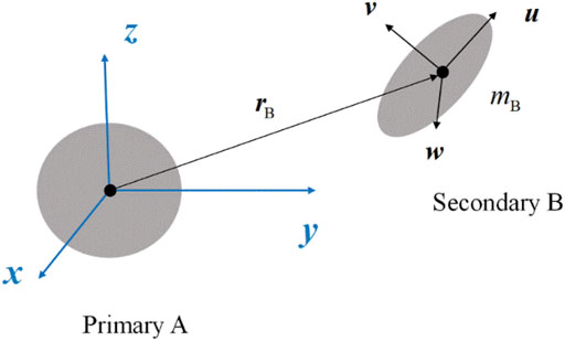
FIGURE 2. Spheroid-ellipsoid two-body configuration.

Then, in the synchronous configuration where ${\mathit{r}}_{\mathrm{B}}$ and $\mathit{u}$ are aligned (see Figure 1), the mutual potential is reduced to

$U\left({\mathit{r}}_{\mathrm{B}}\right)=-\frac{G{m}_{\mathrm{A}}{m}_{\mathrm{B}}}{r_{\mathrm{B}}}+\frac{G{m}_{\mathrm{A}}{m}_{\mathrm{B}}}{2r_{\mathrm{B}}^3}\left[{\tau }_{0A}-3{\tau }_{0A}{\left({\widehat{\mathit{r}}}_{\mathrm{B}}\cdot \mathit{z}\right)}^2+{\tau }_{0B}-6{\tau }_{2B}\right](48)$

Since the relative attitude of the two bodies is fixed (we assume that the slow precession of the mutual orbit does not break this equilibrium configuration), the relative motion of the two bodies, under their mutual gravitation, can be modeled as the perturbed Keplerian two-body problem, in which the perturbation is their non-spherical mutual gravity. The relative motion is governed by

${\ddot{\mathit{r}}}_{\mathrm{B}}=-\frac{{\mu }_{\mathrm{A}\mathrm{B}}}{r_{\mathrm{B}}^2}{\widehat{\mathit{r}}}_{\mathrm{B}}+\frac{3{\mu }_{\mathrm{A}\mathrm{B}}}{2r_{\mathrm{B}}^4}\left\{{\tau }_{0\mathrm{A}}\left[\left(1-5{\left({\widehat{\mathit{r}}}_{\mathrm{B}}\cdot \mathit{z}\right)}^2\right){\widehat{\mathit{r}}}_{\mathrm{B}}+2\left({\widehat{\mathit{r}}}_{\mathrm{B}}\cdot \mathit{z}\right)\mathit{z}\right]+\left({\tau }_{0B}-6{\tau }_{2B}\right){\widehat{\mathit{r}}}_{\mathrm{B}}\right\}(49)$

where ${\mu }_{\mathrm{A}\mathrm{B}}=G\left(m_{\mathrm{A}}+m_{\mathrm{B}}\right)$. Then, we perform averaging over the mutual orbit, and by the Lagrange planetary equations in terms of classical elements, the secular equations of motion are given as

${\dot{a}}_{\mathrm{B}}={\dot{i}}_{\mathrm{B}}={\dot{e}}_{\mathrm{B}}=0(50)$

${\dot{\mathrm{\Omega }}}_{\mathrm{B}}=\frac{3n_{\mathrm{B}}{\tau }_{0\mathrm{A}}}{2a_{\mathrm{B}}^2{\left(1-e_{\mathrm{B}}^2\right)}^2}\cos i_{\mathrm{B}}(51)$

${\dot{\omega }}_{\mathrm{B}}=\frac{3n_{\mathrm{B}}}{4a_{\mathrm{B}}^2{\left(1-e_{\mathrm{B}}^2\right)}^2}{\tau }_{0\mathrm{A}}\left[\left(1-5{\cos }^{}{i}_{\mathrm{B}}\right)-2\frac{{\tau }_{0\mathrm{B}}-6{\tau }_{2\mathrm{B}}}{{\tau }_{0\mathrm{A}}}\right](52)$

As we can see, the shape of the secondary’s orbit is unchanged but its orientation undergoes precession due to the secular evolution of the argument of perigee ${\omega }_{\mathrm{B}}$ and longitude of the ascending node ${\mathrm{\Omega }}_{\mathrm{B}}$. Note that the precession of ${\mathrm{\Omega }}_{\mathrm{B}}$ is caused by the primary’s oblateness, while the evolution of ${\omega }_{\mathrm{B}}$ is a joint effect of the primary’s and secondary’s non-spherical gravity. Given the initial orbital conditions, ${\mathrm{\Omega }}_{\mathrm{B}}$ and ${\omega }_{\mathrm{B}}$ vary linearly with time, and we can easily add them into the particle’s orbital motion equations.

3.2 Equations with the non-spherical third-body gravity

We consider the orbital dynamics around the primary (an oblate spheroid) with the secondary (an ellipsoid) as the perturbing body. As is known, the third-body perturbing acceleration is the difference between the absolute acceleration that the particle feels and the absolute acceleration that the central body feels

${\mathit{a}}_{\mathrm{P}\mathrm{B}}={\mathit{a}}_{\mathrm{B}}-{\mathit{a}}_{\mathrm{B}-\mathrm{A}}(53)$

where ${\mathit{a}}_{\mathrm{B}}$ is given as

$\begin{array}{l}{\mathit{a}}_{\mathrm{B}}=-\frac{{\mu }_{\mathrm{B}}}{{\rho }^2}\widehat{\mathit{\rho }}+\frac{3{\mu }_B{\tau }_{0B}}{2{\rho }^4}\left\{\left[1-5{\left(\widehat{\mathit{\rho }}\cdot \mathit{w}\right)}^2\right]\widehat{\mathit{\rho }}+2\left(\widehat{\mathit{\rho }}\cdot \mathit{w}\right)\mathit{w}\right\}\\ -\frac{3{\mu }_B{\tau }_{2B}}{{\rho }^4}\left\{5\left[{\left(\widehat{\mathit{\rho }}\cdot \mathit{u}\right)}^2-{\left(\widehat{\mathit{\rho }}\cdot \mathit{v}\right)}^2\right]\widehat{\mathit{\rho }}-2\left[\left(\widehat{\mathit{\rho }}\cdot \mathit{u}\right)\mathit{u}-\left(\widehat{\mathit{\rho }}\cdot \mathit{v}\right)\mathit{v}\right]\right\}\end{array}(54)$

in which $\mathit{\rho }=\mathit{r}-{\mathit{r}}_{\mathrm{B}}$; from Eq. 48, ${\mathit{a}}_{\mathrm{B}-\mathrm{A}}$ is given as

${\mathit{a}}_{\mathrm{B}-\mathrm{A}}=\frac{{\mu }_{\mathrm{B}}}{r_{\mathrm{B}}^2}{\widehat{\mathit{r}}}_{\mathrm{B}}-\frac{3{\mu }_{\mathrm{B}}}{2r_{\mathrm{B}}^4}{\tau }_{0\mathrm{A}}\left\{\left[1-5{\left({\widehat{\mathit{r}}}_{\mathrm{B}}\cdot \mathit{z}\right)}^2\right]{\widehat{\mathit{r}}}_{\mathrm{B}}+2\left({\widehat{\mathit{r}}}_{\mathrm{B}}\cdot \mathit{z}\right)\mathit{z}\right\}-\frac{3{\mu }_{\mathrm{B}}}{2r_{\mathrm{B}}^4}\left({\tau }_{0B}-6{\tau }_{2B}\right){\widehat{\mathit{r}}}_{\mathrm{B}}(55)$

For use in perturbation analysis, it is convenient to recast ${\mathit{a}}_{\mathrm{P}\mathrm{B}}$ as a disturbing function

$\begin{array}{l}{R}_{\mathrm{P}\mathrm{B}}=\frac{{\mu }_B}{\left|\mathit{r}-{\mathit{r}}_{\mathrm{B}}\right|}-\frac{{\mu }_B{\tau }_{0B}}{2{\left|\mathit{r}-{\mathit{r}}_{\mathrm{B}}\right|}^3}\left[1-3\frac{{\left(\mathit{r}\cdot \mathit{\gamma }\right)}^2}{{\left|\mathit{r}-{\mathit{r}}_{\mathrm{B}}\right|}^2}\right]+\frac{3{\mu }_B{\tau }_{2B}}{{\left|\mathit{r}-{\mathit{r}}_{\mathrm{B}}\right|}^5}\left[{\left(\left(\mathit{r}-{\mathit{r}}_{\mathrm{B}}\right)\cdot \mathit{\alpha }\right)}^2-{\left(\mathit{r}\cdot \mathit{\beta }\right)}^2\right]\\ -\frac{{\mu }_B}{r_{\mathrm{B}}^2}\left({\widehat{\mathit{r}}}_{\mathrm{B}}\cdot \mathit{r}\right)+\frac{3{\mu }_B{\tau }_{0A}}{2r_{\mathrm{B}}^4}\left\{\left[1-5{\left({\widehat{\mathit{r}}}_{\mathrm{B}}\cdot \mathit{z}\right)}^2\right]\left({\widehat{\mathit{r}}}_{\mathrm{B}}\cdot \mathit{r}\right)+2\left({\widehat{\mathit{r}}}_{\mathrm{B}}\cdot \mathit{z}\right)\left(\mathit{z}\cdot \mathit{r}\right)\right\}\\ +\frac{3{\mu }_B}{2r_{\mathrm{B}}^4}\left({\tau }_{0B}-6{\tau }_{2B}\right)\left({\widehat{\mathit{r}}}_{\mathrm{B}}\cdot \mathit{r}\right)\end{array}(56)$

Substituting $R_{\mathrm{P}\mathrm{B}}$ in Eq. 56 into Eq. 5, we obtain the extended full equations of motion including the non-spherical third-body gravity.

Then, by using Taylor expansion in terms of $\left(r/r_{\mathrm{B}}\right)$ and truncated to the hexadecapole order, the disturbing function is approximated as

$\begin{array}{l}{R}_{\mathrm{P}\mathrm{B}}=-\frac{{\mu }_{\mathrm{B}}}{8r_{\mathrm{B}}}\left\{4{\left(r/r_{\mathrm{B}}\right)}^2\left[3{\left({\widehat{\mathit{r}}}_{\mathrm{B}}\cdot \widehat{\mathit{r}}\right)}^2-1\right]\right.+4{\left(r/r_{\mathrm{B}}\right)}^3\left[5{\left({\widehat{\mathit{r}}}_{\mathrm{B}}\cdot \widehat{\mathit{r}}\right)}^3-3\left({\widehat{\mathit{r}}}_{\mathrm{B}}\cdot \widehat{\mathit{r}}\right)\right]\left.+{\left(r/r_{\mathrm{B}}\right)}^4\left[35{\left({\widehat{\mathit{r}}}_{\mathrm{B}}\cdot \widehat{\mathit{r}}\right)}^4-30{\left({\widehat{\mathit{r}}}_{\mathrm{B}}\cdot \widehat{\mathit{r}}\right)}^2+3\right]\right\}\\ -\frac{3{\mu }_{\mathrm{B}}}{2r_{\mathrm{B}}}\frac{{\tau }_{0\mathrm{A}}r}{r_{\mathrm{B}}^3}\left\{\left[1-5{\left({\widehat{\mathit{r}}}_{\mathrm{B}}\cdot \mathit{z}\right)}^2\right]\left({\widehat{\mathit{r}}}_{\mathrm{B}}\cdot \widehat{\mathit{r}}\right)+2\left({\widehat{\mathit{r}}}_{\mathrm{B}}\cdot \mathit{z}\right)\left(\widehat{\mathit{r}}\cdot \mathit{z}\right)\right\}+\frac{3{\mu }_{\mathrm{B}}}{4r_{\mathrm{B}}}\frac{{\tau }_{0\mathrm{B}}{r}^2}{r_{\mathrm{B}}^4}\left[5{\left({\widehat{\mathit{r}}}_{\mathrm{B}}\cdot \widehat{\mathit{r}}\right)}^2-2{\left(\widehat{\mathit{r}}\cdot \mathit{\gamma }\right)}^2-1\right]\\ -\frac{3{\mu }_{\mathrm{B}}}{2r_{\mathrm{B}}}\frac{{\tau }_{2\mathrm{B}}{r}^2}{r_{\mathrm{B}}^4}\left[17{\left({\widehat{\mathit{r}}}_{\mathrm{B}}\cdot \widehat{\mathit{r}}\right)}^2-2{\left(\widehat{\mathit{r}}\cdot \mathit{\beta }\right)}^2-5\right]\end{array}(57)$

The terms in the first curly brace correspond to the point mass gravity, which is also given in Eq. 3. The other terms are the contributions of the non-spherical gravity of the two massive bodies. As is clear, if the two massive bodies are fairly oblate or elongated, the strength of the primary’s oblateness, represented by ${\tau }_{0\mathrm{A}}$, may be comparable to the point mass’s octupole order, while the secondary’s second degree and order gravity, ${\tau }_{0\mathrm{B}}$ and ${\tau }_{2\mathrm{B}}$, is comparable to the hexadecapole order. However, in general cases, these non-spherical terms are smaller than other terms of the same corresponding order.

Calculating the averaging of these non-spherical terms is similar to those in Section 2.2, and for brevity, we illustrate them in Supplementary Appendix C. Finally, we obtain the extended double-averaged equations of motion as

$\left\{\begin{array}{c}\dot{\mathit{h}}=\kappa {\dot{\mathit{h}}}_{J_2}^{*}+{\dot{\mathit{h}}}_{\mathrm{Q}\mathrm{u}\mathrm{a}}^{*}+\left({\epsilon }_{\mathrm{O}\mathrm{c}\mathrm{t}}{\dot{\mathit{h}}}_{\mathrm{O}\mathrm{c}\mathrm{t}}^{*}+{\epsilon }_{\mathrm{O}\mathrm{c}\mathrm{t}}^{\mathrm{N}}{\dot{\mathit{h}}}_{\mathrm{O}\mathrm{c}\mathrm{t}}^{\mathrm{N}}\right)+\left({\epsilon }_{\mathrm{H}\mathrm{e}\mathrm{x}}{\dot{\mathit{h}}}_{\mathrm{H}\mathrm{e}x}^{*}+{\epsilon }_{\mathrm{H}\mathrm{e}\mathrm{x},0}^{\mathrm{N}}{\dot{\mathit{h}}}_{\mathrm{H}\mathrm{e}\mathrm{x},0}^{\mathrm{N}\ast }+{\epsilon }_{\mathrm{H}\mathrm{e}\mathrm{x},2}^{\mathrm{N}}{\dot{\mathit{h}}}_{\mathrm{H}\mathrm{e}\mathrm{x},2}^{\mathrm{N}\ast }\right)\\ \dot{\mathit{e}}=\kappa {\dot{\mathit{e}}}_{J_2}^{*}+{\dot{\mathit{e}}}_{\mathrm{Q}\mathrm{u}\mathrm{a}}^{*}+\left({\epsilon }_{\mathrm{O}\mathrm{c}\mathrm{t}}{\dot{\mathit{e}}}_{\mathrm{O}\mathrm{c}\mathrm{t}}^{*}+{\epsilon }_{\mathrm{O}\mathrm{c}\mathrm{t}}^{\mathrm{N}}{\dot{\mathit{e}}}_{\mathrm{O}\mathrm{c}\mathrm{t}}^{\mathrm{N}\ast }\right)+\left({\epsilon }_{\mathrm{H}\mathrm{e}\mathrm{x}}{\dot{\mathit{e}}}_{\mathrm{H}\mathrm{e}\mathrm{x}}^{*}+{\epsilon }_{\mathrm{H}\mathrm{e}\mathrm{x},0}^{\mathrm{N}}{\dot{\mathit{e}}}_{\mathrm{H}\mathrm{e}\mathrm{x},0}^{\mathrm{N}\ast }+{\epsilon }_{\mathrm{H}\mathrm{e}\mathrm{x},2}^{\mathrm{N}}{\dot{\mathit{e}}}_{\mathrm{H}\mathrm{e}\mathrm{x},2}^{\mathrm{N}\ast }\right)\end{array}\right.(58)$

where ${\epsilon }_{\mathrm{O}\mathrm{c}\mathrm{t}}^{\mathrm{N}}=-{\tau }_{0A}/a^2\times {\epsilon }_{\mathrm{O}\mathrm{c}\mathrm{t}}$, ${\epsilon }_{\mathrm{H}\mathrm{e}\mathrm{x},0}^{\mathrm{N}}=-{\tau }_{0B}/a^2\times {\epsilon }_{\mathrm{H}\mathrm{e}\mathrm{x}}$, and ${\epsilon }_{\mathrm{H}\mathrm{e}\mathrm{x},2}^{\mathrm{N}}={\tau }_{2B}/a^2\times {\epsilon }_{\mathrm{H}\mathrm{e}\mathrm{x}}$ are the coefficients of the non-spherical effects of the third-body perturbation.

4 Numerical results

We discuss two typical applications in this Section to demonstrate the obtained secular models and compare their performances at different levels of approximation. First, we apply the secular model to a small-scale binary system, the binary asteroid system, where the system is not highly hierarchical, and the high-order terms and the non-spherical gravity of the perturbing body may be significant. Then, we turn to the large-scale astrophysical systems, where the inclination and eccentricity of the perturbing body may have more critical effects than the hexadecapole terms. By the way, a systematic study of the secular dynamics of such systems is complicated and will be the focus of our future work.

4.1 Applications to the binary asteroid systems

The applications to the binary asteroid system 4951 Iwamoto are illustrated as an example to validate our double-averaged model and to present numerical results. Observations indicate that 4951 Iwamoto is a doubly synchronous binary asteroid system with a period of 118 h (Pravec et al., 2016). The diameters of the primary and secondary are inferred to be 5.52 km and 3.34 km, respectively, and the secondary is about 31 km from the primary. Since further information is still unknown, some assumptions are made on the physical and orbital characteristics of the binary system, as shown in Table 1. First, we assume the primary is shaped like an oblate spheroid and the secondary is nearly a tri-axial ellipsoid. Second, the two massive bodies have the equilibrium long-axis configuration, i.e., the secondary is synchronously rotating with the primary lies on its long axis. The secondary is assumed to be in an inclined and eccentric orbit around the primary with $e_{\mathrm{B}}=0.2$ and $i_{\mathrm{B}}=10°$.

TABLE 1

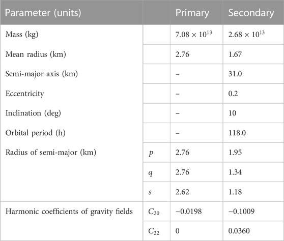
TABLE 1. Parameters of the binary asteroid system 4951 Iwamoto.

The second degree and order gravity coefficients in Table 1 are calculated by (Wang and Fu, 2020)

$C_{20}=\frac{1}{5R_e^2}\left(s^2-\frac{p^2+q^2}{2}\right)(59)$

$C_{22}=\frac{1}{20R_e^2}\left(p^2-q^2\right)(60)$

where s, q, and p are the semi-major axes of an ellipsoid, satisfying $s\le q\le p$.

As stated above, strong perturbations may invalidate the averaging process. It means, for the combined effects of the oblateness of the central body and the gravity of the third body, there are lower and upper limits on the orbit altitude that ensure reliability of the averaging. According to Wang and Fu (2020), for the system parameters given in Table 1, the valid range of the orbit semimajor axis around the primary is about 5.0 km–8.0 km, corresponding to the coefficient $\kappa$ varying from 3.57 to 0.34, as shown in Figure 3. Note that the magnitudes of the octupole order coefficient ${\epsilon }_{\mathrm{O}\mathrm{c}\mathrm{t}}$ and the hexadecapole order coefficient ${\epsilon }_{\mathrm{H}\mathrm{e}\mathrm{x}}$ are about the same order (varying between 0.02 and 0.08), due to the octupole order coefficient having a factor of the perturbing body’s eccentricity $e_{\mathrm{B}}$. Therefore, it is necessary to take both of them into the secular model for the purpose of propagating long-term orbital motion.

FIGURE 3

FIGURE 3. Coefficients of $\kappa$ (left y-axis), and ${\epsilon }_{\mathrm{O}\mathrm{c}\mathrm{t}}$; ${\epsilon }_{\mathrm{H}\mathrm{e}\mathrm{x}}$ (right y-axis) with semimajor axis.

Comparisons are made among the numerical integrations of the four dynamical models: the full, the quadrupole-level, the octupole-level, and the hexadecapole-level models. The full model (non-averaged) given by Eq. 5 is considered to be exact. The other three models are all double averaged but retained to different levels of approximation.

In Figures 4, 5, the orbital evolution over scaled time is depicted, with the semimajor axes set as 5.3 km and 7.8 km respectively (both within the range where the averaging is reliable). The other initial orbital elements are explicitly given in the caption of Figure 4. Actually, they can be chosen arbitrarily for the purpose of demonstrations of the different models. For comparisons of the performance of these models at different orbital altitudes, the initial conditions in Figure 4; Figure 5,; Figure 6 are kept the same except for the semimajor axis. Note that the true time $t$ is related to the scaled time $\tau$ via $t=\tau /{\epsilon }_{\mathrm{P}\mathrm{B}}$ (Eq. 45). The scaled time of 10 in Figures 4, 5 corresponds to the true time of 330.3 days and 188.6 days, respectively. The precession of the secondary’s orbit is incorporated in the numerical integrations of our full and double-averaged models by including the evolution of ${\mathrm{\Omega }}_{\mathrm{B}}$ and ${\omega }_{\mathrm{B}}$ described in Eqs. 51, 52 respectively. Since the semimajor axis is constant in the averaged dynamics, only four remaining orbital elements: eccentricity $e$, inclination $i$, argument of perigee $\omega$, and longitude of ascending node $\mathrm{\Omega }$, need to be considered.

FIGURE 4

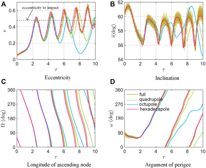
FIGURE 4. Long-term orbital evolution for $a=5.3\mathrm{k}\mathrm{m}$ over 10 scaled time, obtained by models of different approximation levels. The panels (A–D) are the temporal evolution of the eccentricity, inclination, longitude of ascending node, and argument of perigee, respectively. The full model is given by Eq. 5 with $R_{\mathrm{P}\mathrm{B}}$ given in Eq. 56. The other three double-averaged models are given in Eq. 58 (by retaining their corresponding order). The curves of different models are marked by colors (the legend is only given in one of the plots for simplicity). The initial conditions are set as $e_0=0.05$; $i_0={\mathrm{\Omega }}_0=60°$; ${\omega }_0=90°$; ${\mathrm{\Omega }}_0=60°$,; $f_0=0°$ (the initial true anomaly). The secondary’s orbit has $a_B=31\mathrm{k}\mathrm{m}$, $e_B=0.2,i_B=10°$, and ${\Omega }_B={\Omega }_B=f_B=0$. The precession of the secondary’s orbit is governed by Eqs. 51 and 52. The dashed line in the eccentricity figure denotes the critical eccentricity that will cause impact on the surface of the primary.

FIGURE 5

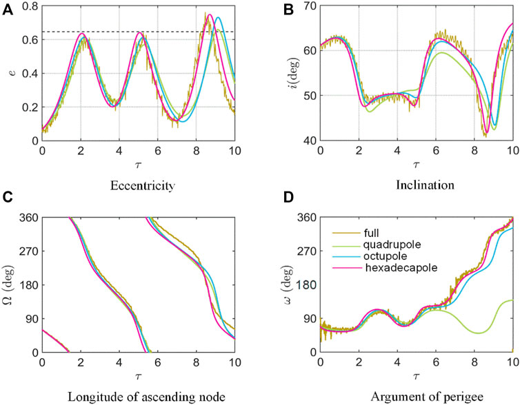
FIGURE 5. Long-term orbital evolution for $a=7.8\mathrm{k}\mathrm{m}$ over 10 scaled time with the other conditions set the same as Figure 4. The panels (A–D) exhibit the temporal evolution of the eccentricity, inclination, longitude of ascending node, and argument of perigee, respectively.

FIGURE 6

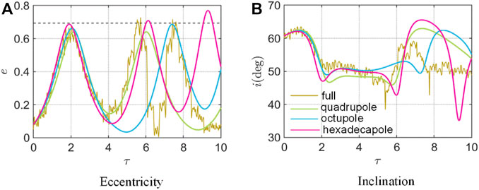
FIGURE 6. Long-term orbital evolution for $a=9.0\mathrm{k}\mathrm{m}$ over 10 scaled time with the other conditions set the same as Figure 4. The panels (A,B) show the temporal evolution of the eccentricity and inclination, respectively.

From Figures 4, 5, we find that within the valid range of orbital altitude, the hexadecapole-level model could well track the secular orbital evolution, while the quadrupole-level and octupole-level models may have significant deviations. However, beyond this range, for example, as shown in Figure 6, when $a=9.0$ km, orbits are strongly perturbed by the third-body gravity and, as a consequence, the large-amplitude short-period oscillation invalidates the averaging processes.

Remember that in the classical Lidov-Kozai mechanism or the extended “$J_2$ included Lidov-Kozai mechanism”, the conservation of vertical-component orbit angular momentum, $h_{\mathit{z}}$, leads to regular, anti-correlated oscillation of the eccentricity and inclination. In the current model, there is a similar anti-correlation behavior between $e$ and $i$, but not regular. In particular, there is a secular effect, as illustrated in Figure 4A, that may force $h_{\mathit{z}}$ to undergo (chaotic) secular changes, resulting in high eccentricities. Recall that in the eccentric Lidov-Kozai effects, the octupole order can modulate the Lidov-Kozai cycles (the secular change of $h_{\mathit{z}}$ can be considered as the Lidov-Kozai cycles undergo secular drift), and thus excite the extremely high eccentricities and even orbit flips (Katz et al., 2011; Lithwick and Naoz, 2011). However, as shown in Figure 7, our results may be a different secular dynamical effect because they are a joint effort of the third-body eccentricity and inclination. It seems that the large eccentricity increases should be attributed to $i_{\mathrm{B}}$, while $e_{\mathrm{B}}$ changes the phase of this secular variation.

FIGURE 7

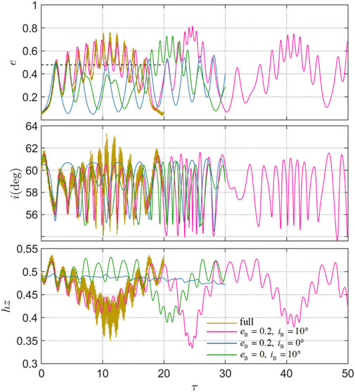
FIGURE 7. Comparisons of the orbital evolution among different combinations of $i_{\mathrm{B}}$ and $e_{\mathrm{B}}$. The full model is integrated to 20 scaled time with $e_{\mathrm{B}}=0.2$ and $i_{\mathrm{B}}=10°$. The other three integrations are all based on the hexadecapole-level model with the scaled integration time: 50 for $e_{\mathrm{B}}=0.2$, $i_{\mathrm{B}}=10°$, and 30 for $e_{\mathrm{B}}=0.2$, $i_{\mathrm{B}}=0$ and $e_{\mathrm{B}}=0$, $i_{\mathrm{B}}=10°$.

In Figure 8, we depict the long-term orbital evolution with different inclinations at $a=5.5$ km. For simplicity, only the eccentricity evolution is displayed. First, we show that the hexadecapole-level model is highly accurate, while the quadrupole-level and octupole-level models have moderate deviations. As we have mentioned above, the system is integrable in the coplanar configuration in the quadrupole-level model, even if the perturbing body is eccentric. For comparisons, we integrate these integrable equations which are obtained by substituting $i_{\mathrm{B}}=0$ into the quadrupole-level model with other parameters remaining unchanged. From Figure 8, we can see the significant differences between the full dynamics and the integrable approximation. In addition, in these integrable cases, the equilibrium points (i.e., frozen orbits) and their stabilities are well-defined. According to Delsate et al. (2010), by using the current system parameters, the analytical unstable inclination interval at $a=5.5$ km is calculated as $55.3°<i<81.9°$ and $100.0°<i<124.4°$, which is symmetric about $i=90°$. However, in the inclined third-body problem, the inclination is different with respect to the central body’s equator and with respect to the third-body orbit plane, especially when the perturbing body’s orbital plane is in precession, as shown in Figure 8. Thus, if we use the solutions of the integrable cases as initial guesses, the unstable inclination regions should be revised according to the specific geometric configuration of the system.

FIGURE 8

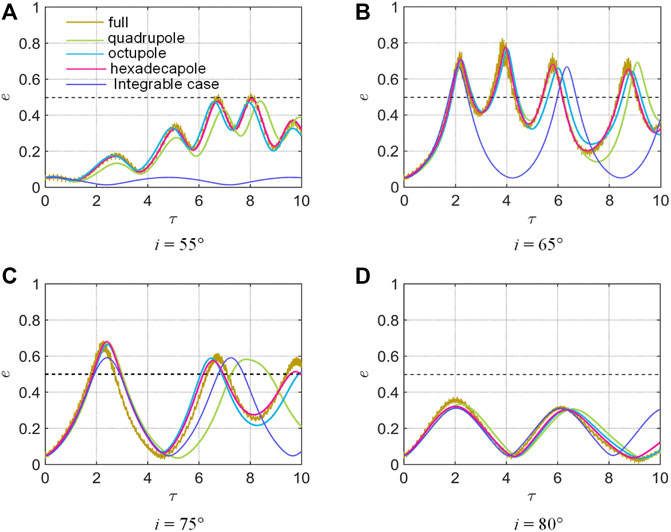
FIGURE 8. Long-term eccentricity evolution at different inclinations for $a=5.5\mathrm{k}\mathrm{m}$ with the other initial conditions set the same as Figure 4. The initial inclinations are set as 55°, 65°, 75°, and 80° in panels (A–D), respectively. The integrable case corresponds to the quadrupole-level model with zero third-body inclination (remaining $e_{\mathrm{B}}$ unchanged).

Then, we show comparisons among these different levels of approximation models for the special cases in which the perturbing body has zero inclination or eccentricity. The corresponding double-averaged equations of motion can be obtained by substituting $e_{\mathrm{B}}=0$ or $i_{\mathrm{B}}=0$ into Eq. 58.

Figure 9 illustrates the case when $i_{\mathrm{B}}=0$ and $e_{\mathrm{B}}=0.2$. For the given initial conditions, the orbit is initially located near a stable Lidov-Kozai equilibrium ($\omega =90°$) solved by the quadrupole-level model. However, in the full and octupole-level (or higher-level) models, the amplitude of the Lidov-Kozai oscillation gradually increases and finally causes an impact on the primary. In addition, although the octupole order and hexadecapole order have similar magnitudes ${\epsilon }_{\mathrm{O}\mathrm{c}\mathrm{t}}\sim {\epsilon }_{\mathrm{H}\mathrm{e}\mathrm{x}}=0.04$, the dramatic, qualitative changes in dynamics only happen when moving from quadrupole-level to octupole-level models. This is because the octupole order recovers the geometric non-axisymmetry of the system, thus eliminating $h_z$ as a constant, leaving only two integrals of motion: the semi-major axis and the double-averaged perturbing potential. That is, there are no other integrals of motion to be eliminated in the higher-level models, and thus no more qualitative changes are expected (Naoz et al., 2013).

FIGURE 9

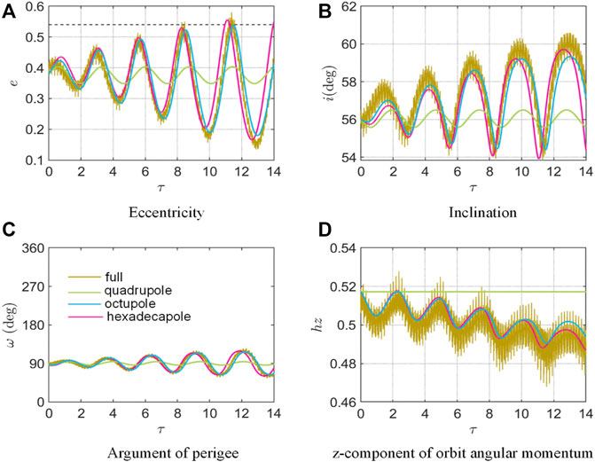
FIGURE 9. Long-term orbital evolution over 14 scaled time with $e_{\mathrm{B}}=0.2$ and $i_{\mathrm{B}}=0$. The initial orbital elements are set as $a_0=6.0$ km, $e_0=0.4$, $i_0=56°$, ${\mathrm{\Omega }}_0=50°$, ${\omega }_0=90°$, and $f_0=300°$. The coefficients $\kappa =1.44$ and ${\epsilon }_{\mathrm{O}\mathrm{c}\mathrm{t}}\sim {\epsilon }_{\mathrm{H}\mathrm{e}\mathrm{x}}=0.04$. Note that the initial orbit is located at the nearby of a Lidov-Kozai equilibrium point. The panels (A–C) show the temporal evolution of the eccentricity, inclination, and argument of perigee, respectively. The evolution of the longitude of node is not shown here. Instead, the variation of the z-component of the orbit angular momentum, $h_z$, is depicted in panel (D).

By using the same initial conditions, we set $e_{\mathrm{B}}=0$ and $i_{\mathrm{B}}=10°$ in Figure 10. In contrast to the eccentric third-body perturbation problem in Figure 9, when $i_{\mathrm{B}}\ne 0$, there are no special integrals of motion in the lowest-order (quadrupole-level) model compared to the higher-level models. Thus, the high order terms may contribute no qualitative changes but quantitatively affect the orbit evolutionary behavior, as shown in Figure 10.

FIGURE 10

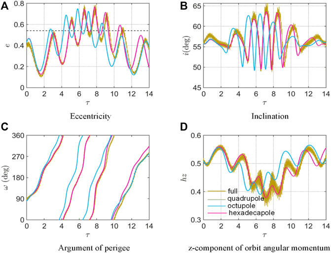
FIGURE 10. Long-term orbital evolution over 14 scaled time with $e_{\mathrm{B}}=0$ and $i_{\mathrm{B}}=10°$. The other initial conditions are set the same as Figure 9. The coefficients $\kappa =1.53$, ${\epsilon }_{\mathrm{O}\mathrm{c}\mathrm{t}}=0$, and ${\epsilon }_{\mathrm{H}\mathrm{e}\mathrm{x}}=0.04$. Since the octupole order coefficient ${\epsilon }_{\mathrm{O}\mathrm{c}\mathrm{t}}=0$, the quadrupole- and octupole-level models are identical. The panels (A–D) show the temporal evolution of the eccentricity, inclination, argument of perigee, and z-component of the orbit angular momentum, respectively.

4.2 Applications to other physical systems

The derived semi-analytical model can also be applied to astrophysical systems covering a wide range of physical scales, such as the exoplanet around an oblate host star with a distant stellar mass or giant planet perturber, where the inner planet can be regarded as massless. Similar dynamical settings have been extensively considered in the eccentric Lidov-Kozai mechanism (Katz et al., 2011; Lithwick and Naoz, 2011; Naoz et al., 2013; Naoz, 2016).

In the scaled dynamical model, Eq. 46, the orbital dynamics can be characterized by three parameters: the oblateness coefficient $\kappa$, the octupole-order coefficient ${\epsilon }_{\mathrm{O}\mathrm{c}\mathrm{t}}$, and the inclination of the third-body orbit $i_{\mathrm{B}}$. Here, we consider two cases: (1) $\kappa =0.1$; ${\epsilon }_{\mathrm{O}\mathrm{c}\mathrm{t}}=0.01$,; $i_{\mathrm{B}}=10°$ in Figure 11, where ${\epsilon }_{\mathrm{O}\mathrm{c}\mathrm{t}}$ is much smaller than $\kappa$; and (2) $\kappa =0.1$, ${\epsilon }_{\mathrm{O}\mathrm{c}\mathrm{t}}=0.1$, and $i_{\mathrm{B}}=10°$ in Figure 12 where ${\epsilon }_{\mathrm{O}\mathrm{c}\mathrm{t}}$ is comparable to $\kappa$.

FIGURE 11

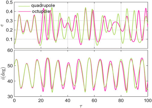
FIGURE 11. Eccentricity and inclination evolution over 100 scaled time for ${\epsilon }_{\mathrm{O}\mathrm{c}\mathrm{t}}=0.01$ by using the quadrupole-level and octupole-level models. The initial orbital elements are $e_0=0.05$, $i_0=50°$, ${\mathrm{\Omega }}_0=60°$ and ${\omega }_0=0$. The perturbing body’s orbit is assumed to be fixed at ${\omega }_{\mathrm{B}}={\mathrm{\Omega }}_{\mathrm{B}}=0°$.

FIGURE 12

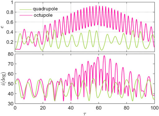
FIGURE 12. Eccentricity and inclination evolution over 100 scaled time for ${\epsilon }_{\mathrm{O}\mathrm{c}\mathrm{t}}=0.1$ by using the quadrupole-level and octupole-level models. The other conditions are set the same as Figure 11.

From Figures 11, 12, we show the important role of the octupole-order terms, especially when the octupole-order coefficient ${\epsilon }_{\mathrm{O}\mathrm{c}\mathrm{t}}$ is comparable to the oblateness-related coefficient $\kappa$ (Figure 12), which may lead to the dramatic, qualitatively different evolutionary behaviors. We note that the secular effect shown in Figure 12 is different from that in Figure 7 because the orbit inclination oscillates in a small range even when the orbit reaches high eccentricities in Figure 7, while in Figure 12, the large increases in eccentricities are accompanied by wide excursions of inclination. We suppose that these two secular effects may be the mechanism of forming close-in exoplanets of different inclination types. However, the detailed analysis is beyond the scope of our current work, which will be focused on in our future work.

5 Conclusion

Previous studies have revealed the striking features induced by the octupole-order approximation of the third-body perturbation (Katz et al., 2011; Lithwick and Naoz, 2011; Naoz, 2016) and the notable effects caused by the third-body inclination (Yokoyama, 1999; Liu et al., 2012; Nie and Gurfil, 2021), separately, in the hierarchical restricted three-body problem. We find that in some astrophysical and astrodynamical systems, the two factors may be simultaneously significant (Winn and Fabrycky, 2015). Concerning this, in this paper, we have developed a semi-analytical model to provide effective tools for the solution of this problem. Our model includes the perturbations of the central body’s oblateness and the third-body gravity to the hexadecapole order. In particular, the perturbing body is assumed to be in an inclined and eccentric orbit and its non-spherical gravity is also incorporated. Thanks to the double averaging, the secular dynamics can be parameterized by a few coefficients, and through which one can conduct analytical studies on a wide range of physical systems. Formulated in vectorial elements, the equations of motion take a compact form and can be easily reduced to the coplanar or circular perturbing body cases.

Then, numerical integrations have been proposed to demonstrate the validity of our model and to present some numerical results. Comparisons are made among the full, quadruple-level, octupole-level, and hexadecapole-level models. From the numerical results applied to the binary asteroid system 4951 Iwamoto, we have shown the high accuracy of the hexadecapole-level model within the determined valid range of the semimajor axis, while the quadrupole-level and octupole-level models may have obvious deviations. In addition, several secular dynamical features have been highlighted: (a) a joint effect of the perturbing body’s inclination and eccentricity that could drive high eccentricities with chaotic behavior (see Figure 7); (b) the changes in the unstable inclination regions due to the third-body inclination (see Figure 8); and (c) for the $i_{\mathrm{B}}=0$ cases, the octupole-order terms may break the stable Lidov-Kozai equilibrium points by gradually increasing their amplitudes (see Figure 9). We have also integrated a fictitious system with assumed parameters. We have found that when the coefficient $\kappa$ is comparable to the octupole-order coefficient ${\epsilon }_{\mathrm{O}\mathrm{c}\mathrm{t}}$, the octupole-order terms may bring new secular effects that could excite both high inclinations and high eccentricities (see Figure 12). We point out that a thorough study of dynamical essence of these secular features is beyond the scope of this paper, which will be the motivation for our future work.

Data availability statement

The raw data supporting the conclusions of this article will be made available by the authors, without undue reservation.

Author contributions

TF derived the equations, did the calculations, and wrote the manuscript; YW made the research plan, checked the equations and results, and revised the paper; WH reviewed the paper and gave some suggestions.

Funding

This work was supported by the National Natural Science Foundation of China (Grant number 11872007).

Conflict of interest

The authors declare that the research was conducted in the absence of any commercial or financial relationships that could be construed as a potential conflict of interest.

Publisher’s note

All claims expressed in this article are solely those of the authors and do not necessarily represent those of their affiliated organizations, or those of the publisher, the editors and the reviewers. Any product that may be evaluated in this article, or claim that may be made by its manufacturer, is not guaranteed or endorsed by the publisher.

Supplementary material

The Supplementary Material for this article can be found online at: https://www.frontiersin.org/articles/10.3389/fspas.2023.1125386/full#supplementary-material

References

Allan, R. R., and Cook, G. E. (1963). The long-period motion of the plane of a distant circular orbit. Proc. R. Soc. 280, 97. doi:10.1098/rspa.1964.0133

CrossRef Full Text | Google Scholar

Bellerose, J., and Scheeres, D. J. (2008). Restricted full three-body problem: Application to binary system 1999 KW4. J. Guid. Control. Dyn. 31, 162–171. doi:10.2514/1.30937

CrossRef Full Text | Google Scholar

Broucke, R. A. (2003). Long-term third-body effects via double averaging. J. Guid. Control. Dyn. 26, 27–32. doi:10.2514/2.5041

CrossRef Full Text | Google Scholar

Carvalho, J. P. S., Mourão, D. C., de Moraes, R. V., Prado, A. F. B. A., and Winter, O. C. (2016). Exoplanets in binary star systems: On the switch from prograde to retrograde orbits. Celest. Mech. Dyn. Astron. 124, 73–96. doi:10.1007/s10569-015-9650-3

CrossRef Full Text | Google Scholar

Carvalho, J. P. S., Yokoyama, T., and Mourão, D. C. (2022). Single-averaged model for analysis of frozen orbits around planets and moons. Celest. Mech. Dyn. Astron. 134, 35. doi:10.1007/s10569-022-10092-6

CrossRef Full Text | Google Scholar

Chappaz, L., and Howell, K. C. (2015). Exploration of bounded motion near binary systems comprised of small irregular bodies. Celest. Mech. Dyn. Astron. 123, 123–149.

CrossRef Full Text | Google Scholar

Circi, C., Condoleo, E., and Ortore, E. (2017). A vectorial approach to determine frozen orbital conditions. Celest. Mech. Dyn. Astron. 128, 361–382. doi:10.1007/s10569-017-9757-9

CrossRef Full Text | Google Scholar

Condoleo, E., Cinelli, M., Ortore, E., and Circi, C. (2016). Frozen orbits with equatorial perturbing bodies: The case of ganymede, callisto, and titan. J. Guid. Control. Dyn. 39, 2264–2272. doi:10.2514/1.g000455

CrossRef Full Text | Google Scholar

Ćuk, M., and Nesvorny, D. (2010). Orbital evolution of small binary asteroids. Icarus 207, 732–743. doi:10.1016/j.icarus.2009.12.005

CrossRef Full Text | Google Scholar

De Moraes, R. V., Domingos, R. C., and De Almeida Prado, A. F. B. (2008). Third-body perturbation in the case of elliptic orbits for the disturbing body. Math. Probl. Eng. 2008, 68.

CrossRef Full Text | Google Scholar

Dell’Elce, L., Baresi, N., Naidu, S. P., Benner, L. A. M., and Scheeres, D. J. (2017). Numerical investigation of the dynamical environment of 65803 Didymos. Adv. Sp. Res. 59, 1304–1320. doi:10.1016/j.asr.2016.12.018

CrossRef Full Text | Google Scholar

Delsate, N., Robutel, P., Lemaître, A., and Carletti, T. (2010). Frozen orbits at high eccentricity and inclination: Application to mercury orbiter. Celest. Mech. Dyn. Astron. 108, 275–300. doi:10.1007/s10569-010-9306-2

CrossRef Full Text | Google Scholar

Fu, T., and Wang, Y. (2021). Orbital stability around the primary of a binary asteroid system. J. Guid. Control. Dyn. 44, 1607–1620. doi:10.2514/1.g005832

CrossRef Full Text | Google Scholar

Jacobson, S. A. (2011). Dynamics of rotationally fissioned asteroids: Source of observed small asteroid systems. Icarus 214, 161–178. doi:10.1016/j.icarus.2011.04.009

CrossRef Full Text | Google Scholar

Kamel, A., and Tibbitts, R. (1973). Some useful results on initial node locations for near-equatorial circular satellite orbits. Celest. Mech. 8, 45–73. doi:10.1007/bf01228389

CrossRef Full Text | Google Scholar

Katz, B., Dong, S., and Malhotra, R. (2011). Long-term cycling of kozai-lidov cycles: Extreme eccentricities and inclinations excited by a distant eccentric perturber. Phys. Rev. Lett. 107, 181101. doi:10.1103/physrevlett.107.181101

PubMed Abstract | CrossRef Full Text | Google Scholar

Kinoshita, H., and Nakai, H. (1999). Celest. Mech. Dyn. Astron. 75, 125–147. doi:10.1023/a:1008321310187

CrossRef Full Text

Kinoshita, H., and Nakai, H. (2007). General solution of the Kozai mechanism. Celest. Mech. Dyn. Astron. 98, 67–74. doi:10.1007/s10569-007-9069-6

CrossRef Full Text | Google Scholar

Kinoshita, H., and Nakai, H. (1991). Secular perturbations of fictitious satellites of uranus. Celest. Mech. Dyn. Astron. 52, 293–303. doi:10.1007/bf00048489

CrossRef Full Text | Google Scholar

Kozai, Y. (1969). Long-range variations of orbits with arbitrary inclination and eccentricity. Vistas Astron 11, 103–117. doi:10.1016/0083-6656(69)90006-3

CrossRef Full Text | Google Scholar

Kozai, Y. (1962). Secular perturbations of asteroids with high inclination and eccentricity. Astron. J. 67, 591. doi:10.1086/108790

CrossRef Full Text | Google Scholar

Lara, M., and Juan, J. F. S. (2005). Dynamic behavior of an orbiter around europa. J. Guid. Control. Dyn. 28, 291–297. doi:10.2514/1.5686

CrossRef Full Text | Google Scholar

Lara, M., Rosengren, A. J., and Fantino, E. (2020). Nonsingular recursion formulas for third-body perturbations in mean vectorial elements. Astron. Astrophys. 634, A61. doi:10.1051/0004-6361/201937106

CrossRef Full Text | Google Scholar

Li, G., Dai, F., and Becker, J. (2020). Mutual inclination excitation by stellar oblateness. Astrophys. J. 890, L31. doi:10.3847/2041-8213/ab72f4

CrossRef Full Text | Google Scholar

Li, G., Naoz, S., Holman, M., and Loeb, A. (2014). Chaos in the test particle eccentric kozai–lidov mechanism. Astrophys. J. 791, 86. doi:10.1088/0004-637x/791/2/86

CrossRef Full Text | Google Scholar

Li, X., Qiao, D., and Jia, F. (2021). Investigation of stable regions of spacecraft motion in binary asteroid systems by terminal condition maps. J. Astronaut. Sci. 68, 891–915. doi:10.1007/s40295-021-00296-7

CrossRef Full Text | Google Scholar

Lidov, M. L. (1963). “On the approximated analysis of the orbit evolution of artificial satellites,” in Dynamics of Satellites/Dynamique des Satellites (Berlin, Heidelberg: Springer), 168–179.

CrossRef Full Text | Google Scholar

Lithwick, Y., and Naoz, S. (2011). The eccentric kozai mechanism for a test particle. Astrophys. J. 742, 94. doi:10.1088/0004-637X/742/2/94

CrossRef Full Text | Google Scholar

Liu, X., Baoyin, H., and Ma, X. (2010). Five special types of orbits around mars. Guid. Control. Dyn. 33, 1294–1301. doi:10.2514/1.48706

CrossRef Full Text | Google Scholar

Liu, X., Baoyin, H., and Ma, X. (2012). Long-term perturbations due to a disturbing body in elliptic inclined orbit. Space Sci. 339, 295–304. doi:10.1007/s10509-012-1015-8

CrossRef Full Text | Google Scholar

Lubow, S. H. (2021). An analytic solution to the Kozai–Lidov evolution equations. Mon. Not. R. Astron. Soc. 507, 367–373. doi:10.1093/mnras/stab2133

CrossRef Full Text | Google Scholar

Moe, M., and Kratter, K. M. (2021). Impact of binary stars on planet statistics – I. Planet occurrence rates and trends with stellar mass. Mon. Not. R. Astron. Soc. 507, 3593–3611. doi:10.1093/mnras/stab2328

CrossRef Full Text | Google Scholar

Naoz, S., Farr, W. M., Lithwick, Y., and Rasio, F. A. (2011). Hot Jupiters from secular planet–planet interactions. Nature 473, 187–189. doi:10.1038/nature10076

PubMed Abstract | CrossRef Full Text | Google Scholar

Naoz, S., Farr, W. M., Lithwick, Y., Rasio, F. A., and Teyssandier, J. (2013). Secular dynamics in hierarchical three-body systems. Mon. Not. R. Astron. Soc. 431, 2155–2171. doi:10.1093/mnras/stt302

CrossRef Full Text | Google Scholar

Naoz, S. (2016). The eccentric kozai-lidov effect and its applications. Annu. Rev. Astron. Astrophys. 54, 441–489. doi:10.1146/annurev-astro-081915-023315

CrossRef Full Text | Google Scholar

Nie, T., and Gurfil, P. (2021). Long-term evolution of orbital inclination due to third-body inclination. Celest. Mech. Dyn. Astron. 133, 1. doi:10.1007/s10569-020-09997-x

CrossRef Full Text | Google Scholar

Nie, T., Gurfil, P., and Zhang, S. (2019). Semi-analytical model for third-body perturbations including the inclination and eccentricity of the perturbing body. Celest. Mech. Dyn. Astron. 131, 1. doi:10.1007/s10569-019-9905-5

CrossRef Full Text | Google Scholar

Pravec, P., Scheirich, P., Kusnirak, P., Hornoch, K., Galad, A., Naidu, S. P., et al. (2016). Binary asteroid population. 3. Secondary rotations and elongations. Icarus 267, 267. doi:10.1016/j.icarus.2015.12.019

CrossRef Full Text | Google Scholar

Rosengren, A. J. (2014). Ann and H. J. Smead aerospace engineering Sciences. PhD thesis. (Denver: Univ. Colorado).

Google Scholar

Rosengren, A. J., and Scheeres, D. J. (2013). Long-term dynamics of high area-to-mass ratio objects in high-Earth orbit. Adv. Sp. Res. 52, 1545–1560. doi:10.1016/j.asr.2013.07.033

CrossRef Full Text | Google Scholar

Scheeres, D. J., Guman, M. D., and Villac, B. F. (2001). Stability analysis of planetary satellite orbiters: Application to the europa orbiter. J. Guid. Control. Dyn. 24, 778–787. doi:10.2514/2.4778

CrossRef Full Text | Google Scholar

Scheeres, D. J. (2013). Stability of relative equilibria in the full two-body problem. Ann. N. Y. Acad. Sci. 1017, 81–94. doi:10.1196/annals.1311.006

CrossRef Full Text | Google Scholar

Shi, Y., Wang, Y., Misra, A. K., and Xu, S. (2020). Station-keeping for periodic orbits near strongly perturbed binary asteroid systems. J. Guid. Control. Dyn. 43, 319–326. doi:10.2514/1.g004638

CrossRef Full Text | Google Scholar

Shi, Y., Wang, Y., and Xu, S. (2019). Global search for periodic orbits in the irregular gravity field of a binary asteroid system. Acta Astronaut. 163, 11–23. doi:10.1016/j.actaastro.2018.10.014

CrossRef Full Text | Google Scholar

Šidlichovskyý, M. (1983). Quaternions for regularizing celestial mechanics: The right way. Celest. Mech. 29, 295.

Google Scholar

Spalding, C., and Millholland, S. C. (2020). Stellar oblateness versus distant giants in exciting kepler planet mutual inclinations. Astron. J. 160, 105. doi:10.3847/1538-3881/aba629

CrossRef Full Text | Google Scholar

Tokovinin, A. (2014). From binaries to multiples. II. Hierarchical multiplicity of F and G dwarfs. Astron. J. 147, 87. doi:10.1088/0004-6256/147/4/87

CrossRef Full Text | Google Scholar

Ulivieri, C., Circi, C., Ortore, E., Bunkheila, F., and Todino, F. (2013). Frozen orbital plane solutions for satellites in nearly circular orbit. J. Guid. Control. Dyn. 36, 935–945. doi:10.2514/1.59734

CrossRef Full Text | Google Scholar

Wang, H. S., and Hou, X. Y. (2020). On the secondary’s rotation in a synchronous binary asteroid. Mon. Not. R. Astron. Soc. 493, 171–183. doi:10.1093/mnras/staa133

CrossRef Full Text | Google Scholar

Wang, J., Fischer, D. A., Horch, E. P., and Xie, J. W. (2015). Influence of stellar multiplicity on planet formation. Iii. Adaptive optics imaging ofkeplerstars with gas giant planets. Astrophys. J. 806, 248. doi:10.1088/0004-637x/806/2/248

CrossRef Full Text | Google Scholar

Wang, Y., and Fu, T. (2020). Semi-analytical orbital dynamics around the primary of a binary asteroid system. Mon. Not. R. Astron. Soc. 495, 3307–3322. doi:10.1093/mnras/staa1229

CrossRef Full Text | Google Scholar

Wang, Y., and Gurfil, P. (2016). Dynamical modeling and lifetime analysis of geostationary transfer orbits. Acta Astronaut. 128, 262–276. doi:10.1016/j.actaastro.2016.06.050

CrossRef Full Text | Google Scholar

Wang, Y., Luo, X., and Wu, X. (2020). Long-term evolution and lifetime analysis of geostationary transfer orbits with solar radiation pressure. Acta Astronaut. 175, 405–420. doi:10.1016/j.actaastro.2020.06.007

CrossRef Full Text | Google Scholar

Will, C. M. (2017). Orbital flips in hierarchical triple systems: Relativistic effects and third-body effects to hexadecapole order. Phys. Rev. D. 96, 023017. doi:10.1103/PhysRevD.96.023017

CrossRef Full Text | Google Scholar

Winn, J. N., and Fabrycky, D. C. (2015). The occurrence and architecture of exoplanetary systems. Annu. Rev. Astron. Astrophys. 53, 409–447. doi:10.1146/annurev-astro-082214-122246

CrossRef Full Text | Google Scholar

Yokoyama, T. (1999). Dynamics of some fictitious satellites of Venus and Mars. Space Sci. 47, 619–627. doi:10.1016/s0032-0633(98)00110-x

CrossRef Full Text | Google Scholar

Zhang, R., Wang, Y., Shi, Y., and Xu, S. (2020). Libration points and periodic orbit families near a binary asteroid system with different shapes of the secondary. Acta Astronaut. 177, 15–29. doi:10.1016/j.actaastro.2020.07.006

CrossRef Full Text | Google Scholar