Numerical modeling of solar wind and coronal mass ejection in the inner heliosphere: A review

The predictions of plasma parameters in the interplanetary medium are the core of space weather forecasts, and the magnetohydrodynamics (MHD) numerical simulation is an important tool in the prediction of plasma parameters. Operational space weather forecasts are commonly produced by a heliosphere model whose inner boundary is set at 18 R_s or beyond. Such predictions typically use empirical/physics-based inner boundary conditions to solve the MHD equations for numerical simulation. In recent years, significant progress has been made in the numerical modeling of the inner heliosphere. In this paper, the numerical modeling of solar wind and coronal mass ejection in the inner heliosphere is reviewed. In particular, different inner boundary conditions used in the simulation are investigated since the MHD solutions are predetermined by the treatment of the inner boundary conditions to a large extent. Discussion is made on further development of the heliosphere model.

1 Introduction

Over the past few decades, the effects of space weather on technology have become an important field of research. The most serious space weather impact in near-Earth space is usually related to interplanetary coronal mass ejections (ICMEs), which are affected by the surrounding solar wind when propagated to Earth orbit (Wu et al., 2006; Kilpua et al., 2019; Li et al., 2020). For this reason, solar wind condition is a necessary prerequisite for the propagation of CMEs, which governs the propagation of ICMEs in the interplanetary space. The prediction of solar wind and ICME plasma properties plays a crucial role in the space weather forecast. However, the in situ observations of plasma parameters are only applicable to several points where spacecraft are located, for example, the Advanced Composition Explorer (ACE) (Stone et al., 1998), Wind (Bochsler et al., 1995), Parker Solar Probe (PSP) (Fox et al., 2016), Solar Orbiter (SO) (Müller et al., 2020), and Solar Terrestrial Relations Observatory (STEREO) spacecraft (Howard et al., 2008; Kaiser et al., 2008). Therefore, we have to rely on numerical technology to predict the plasma parameters.

Currently, a wide variety of techniques have been developed to generate plasma parameters in the interplanetary space. In particular, magnetohydrodynamics (MHD) simulations are important tools in this endeavor (Pizzo, 1982; Usmanov, 1993; Odstrcil, 2003; Detman et al., 2006; Nakamizo et al., 2009; Hayashi, 2012; Riley et al., 2012; Feng et al., 2014; Zhang and Feng, 2015; Shiota and Kataoka, 2016; Zhang and Xueshang, 2016; Pomoell and Poedts, 2018; Shen et al., 2018; Scolini et al., 2019; Feng, 2020; Scolini et al., 2020; Singh et al., 2020). The MHD simulations can be classified into two types: the full physics-based models and the hybrid empirical/physics-based models. The full physics-based models solve the MHD simulation from the solar surface to 1 au or beyond, and on the other hand, the inner boundary of the hybrid empirical/physics-based models is usually beyond the corona region, with a set of empirical formulas to specify the solar wind distribution at the lower boundary. Since the plasma β in the lower corona is low, the time step determined by the Courant–Friedrichs–Levy condition is small in the corona region. In this sense, the full physics-based models are computationally expensive and the hybrid empirical/physics-based models have their merits from the perspective of forecasting application because of the inexpensive computational cost and relative simplicity of implementation. Also, Owens et al. (2008) showed that the hybrid empirical/physics-based MHD model can reproduce large-scale solar wind structures comparable with the full physics-based models. The purpose of this study is to review the development status of numerical simulation for solar wind and coronal mass ejection in the inner heliosphere, and in particular, we investigate the different inner boundary conditions used in the models.

2 Numerical simulation of solar wind in the inner heliosphere

The lower boundary of the heliospheric models is usually located around 0.1 au, where the solar wind becomes supersonic and super-Alfvénic. Thus, the MHD solutions are predetermined by the treatment of the inner boundary conditions to a large extent. Different kinds of lower-boundary conditions existed in the inner heliosphere models.

In general, the radial component of the magnetic field B_r at the lower boundary of the heliospheric models is usually obtained by the potential field source surface (PFSS) model (Altschuler and Newkirk, 1969; Schatten et al., 1969; Mackay and Yeates, 1999). In the PFSS model, a source surface (around 2.5 R_s) is defined, and the magnetic field between the solar surface and the source surface is assumed to be current-free and becomes open and purely radial above the source surface. With the magnetograph observations of the photosphere as the input, the PFSS model can rapidly extrapolate the large-scale coronal magnetic structures with reasonable accuracy. However, magnetic fields derived from the PFSS model have no thin heliospheric current sheet (HCS) or Parker spiral in the interplanetary space. To solve this problem, some authors combined the PFSS model with the Schatten current sheet (SCS) model (Schatten, 1971). The SCS model takes the absolute value of the (radial) field on the source surface obtained from the PFSS solution as a new lower-boundary condition, the new potential field is solved between the source surface and infinity, and then, the proper sign is restored. Another method for reconstructing the coronal magnetic field is the current sheet source surface (CSSS) model (Zhao and Hoeksema, 1995) that explicitly takes into account additional sheet currents. The CSSS model includes a cusp surface height R_CS and a source surface height R_SS, where the magnetic field becomes open above R_CS and becomes radial above R_SS. The Ulysses observations show that the strength of the interplanetary magnetic field B_r has no dependence on latitude. However, the large-scale structures of the coronal magnetic field derived from the PFSS model have a systematic gradient of B_r in the latitudinal direction. The CSSS model can better reproduce the latitude-invariant nature of B_r.

Based on the coronal magnetic topology parameters obtained from the previous models, the Wang–Sheeley (WS) or Wang–Sheeley–Arge (WSA)-type models (Arge and Pizzo, 2000; Arge et al., 2004; Mcgregor et al., 2011) are the most widely used empirical models that predict the solar wind velocity at the lower boundary. The specific form of V_r (km/s) in the WS model can be written as

$V_r\left(f_s\right)=V_{\text{min}}+\frac{V_{\text{max}}}{f_s^{\alpha }},(1)$

where f_s is the magnetic expansion factor which reads $f_s={(\frac{1}{R})}^2\frac{B_{R_s}}{B_R}$, where $B_{R_s}$ and B_R are the magnetic field strength at the solar surface and at the source surface, respectively. The distribution of f_s at the lower boundary of the heliospheric models is the same as its distribution at the source surface. V_min sets the minimum possible solar wind speed, while V_max sets the maximum possible solar wind speed. α determines the effect of f_s on V_r. By including an additional variable θ_b, the specific form of V_r (km/s) in the WSA model can be written as

$V_r\left(f_s,{\theta }_b\right)=V_{\text{min}}+\frac{V_{\text{max}}}{{\left(1+f_s\right)}^{a_1}}{\left[1-0.8\text{exp}\left(-{\left(\frac{{\theta }_b}{a_2}\right)}^{a_3}\right)\right]}^{a_4},(2)$

where θ_b denotes the minimum angular separation between an open-field foot point and its nearest coronal hole boundary. The angle a₂ and exponent a₃ determine the angular extent and influence of the open-flux boundary layer, respectively. Any of the parameters in Eqs 1, 2 can be modified.

The other components of the magnetic field and velocity, such as the meridional magnetic field B_θ and the meridional flow velocity V_θ, are always set to 0. The azimuthal flow velocity V_ϕ is always set to zero in the inertial frame and set as Ω_sR_gb sin θ in the rotating frame, with Ω_s denoting the solar angular speed and R_gb standing for the lower boundary of the heliospheric models. The azimuthal magnetic field B_ϕ is determined by B_ϕ = (B_r/V_r) (V_ϕ − Ω_sR_gb sin θ). Other solar wind parameters, including the density and temperature, are always prescribed by an assumption of the constant momentum flux and total pressure (sum of thermal and magnetic pressures). In the following section, the lower-boundary conditions in the existing inner heliospheric models are introduced in detail.

2.1 Boundary conditions based on the PFSS model

Using the PFSS + WS model, Odstrcil (2003) modeled the ambient solar wind from 0.1 au to 1 au using the WS-ENLIL mode. The solar wind velocity at 0.1 au was calculated according to Equation 1 with V_min = 285 km/s, V_max = 575 km/s, and α = 1/1.7. The mass density ρ was determined by an assumption of the constant momentum flux, and the temperature T was chosen to assure the total pressure is uniform on the source surface. Hayashi (2003) reconstructed three-dimensional solar wind structure from 50 R_s to 1 au. The radial flow velocity V_r at the inner boundary was determined by solar wind data obtained from interplanetary scintillation (IPS) observations, and the number density and temperature were determined by the empirical relation obtained from the Helios data through least-squares fitting, $N(V_r)=62.98+866.4{(\frac{V_r-154.9}{100})}^{-3.402}$ and $T(V_r)=-0.455+\frac{0.1943V_r}{100}$. They found that the solar wind research and space weather prediction algorithms can be enhanced by the combination of MHD simulation and IPS tomography. Based on that work, Hayashi (2012) modeled time-dependent solar wind from 50 R_s up to 1,250 R_s. The solar wind was simulated with the time-dependent boundary condition. They applied temporal linear interpolation from one Carrington rotation to the next Carrington rotation. Shiota et al. (2014) developed an inner heliospheric MHD solar wind model for practical use in real-time space weather forecasting. The numerical domain was set to 25R_s ≤ r ≤ 425R_s. The radial flow velocity was determined using Equation 1 with V_min = 267.5 km/s, V_max = 410 km/s, and α = 0.4. The number density and temperature were obtained using empirical relationships that have been used by Hayashi (2003) and Hayashi (2012), respectively. Since Hayashi (2003) and Hayashi (2012) showed the relation at 50 R_s, their model specified the boundary condition at 25 R_s. For modification, the number density was multiplied by 4 assuming constant velocity propagation from 25 R_s to 50 R_s, and the temperature was multiplied by 4^γ−1 with the assumption of polytropic expansion.

Based on the PFSS + WSA model, Merkin et al. (2011); Pahud et al. (2012); and Merkin et al. (2016) simulated the solar wind from 0.1 au to 1 au or beyond using the Lyon–Fedder–Mobarry (LFM) MHD simulation code. This new version of the code is referred to as LFM-helio. The values of V_r at the inner boundary were all calculated according to Equation 2 but with different parameters. In Merkin et al. (2011), V_min = 200 km/s, V_max = 750 km/s, a₁ = 2/9, a₂ = 3.8°, a₃ = 3.6, and a₄ = 3. The number density and temperature were determined by using an empirical fit to Helios data: $N[{\mathrm{c}\mathrm{m}}^{-3}]=112.64+9.49\cdot 10^7/{(V_r[km/s])}^2$, T = N₀T₀/N, where T₀ = 8 ⋅ 10⁵ K and N₀ = 300cm⁻³. Figure 1 shows the radial velocity and magnetic field at the inner boundary of the simulation (0.1 au) (Merkin et al., 2011). The magnetic field at 0.1 au was scaled down by a factor 2/3 × 100.

FIGURE 1

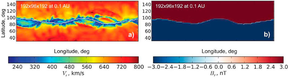
FIGURE 1. Radial velocity (A) and magnetic field (B) at the inner boundary of the simulation (0.1 au) (Merkin et al., 2011).

The inner boundary conditions used by Pahud et al. (2012) were similar to those used by Merkin et al. (2011), except for the following parameters: V_min = 240 km/s, V_max = 675 km/s, a₁ = 2/9, a₂ = 2.8°, a₃ = 1.25, and a₄ = 3. By comparing the MHD results with MESSENGER and ACE spacecraft observations, Pahud et al. (2012) found that the uncertainty in the specification of the boundary conditions, rather than a poor performance of the solar wind model, led to the discrepancies between in situ measurements and simulations. Merkin et al. (2016) used the LFM-helio MHD model to explore the heliospheric consequences of time-dependent changes at the Sun. The Air Force Data Assimilate Photospheric flux Transport (ADAPT) model was used to obtain daily updated photospheric magnetograms. These time-dependent magnetograms were then used to obtain the solar wind parameters at 21.5 R_s with the WSA model. In particular, the changes of the longitudinal and latitudinal components of the magnetic field at the inner boundary were induced by the tangential electric fields, which were derived by a Poisson equation. The V_r at the inner boundary was calculated according to Equation 2 with V_min = 240 km/s, V_max = 675 km/s, a₁ = 2/9, a₂ = 1.9°, a₃ = 2, and a₄ = 3. The number density was determined in the same way as in Merkin et al. (2011). The temperature was defined from the approximate full pressure balance in the angular directions.

$NkT+\frac{B_r^2}{8\pi }=N_{\text{slow}}k{T}_{\text{slow}},(3)$

where k is the Boltzmann constant, N_slow = max(N), and T_slow = 5 ⋅ 10⁵ K is the nominal slow wind plasma temperature. In some cases, one can specify the fast wind temperature parameter T_fast instead to avoid a negative temperature:

$NkT+\frac{B_r^2}{8\pi }=N^{\star }k{T}_{\text{fast}}+\frac{B_{\max }^2}{8\pi },(4)$

where T_fast = 10⁶ K, B_max is the maximum magnetic field located somewhere in the fast solar wind, and N^⋆ represents the plasma density at that location.

Shen et al. (2018) and Wang et al. (2020) used a new boundary treatment to model the solar wind in interplanetary space with MHD equations. The magnetic field was derived by the PFSS model combining with the OMNI database.

$B_r=\text{sign}\left(B^{\text{PFSS}}\right)\times \frac{1}{\sqrt{2}}\mathrm{m}\mathrm{e}\mathrm{a}\mathrm{n}\left(B^{1\text{\hspace{0.17em}au}}\right){\left(\frac{\mathrm{1}\mathrm{a}\mathrm{u}}{R_{gb}}\right)}^2,(5)$

where R_gb = 0.1 au. The average value of the observed magnetic field, mean (B^{1 au}), was determined by the past three Carrington rotations (CRs) at 1 au from the OMNI database. The solar wind velocity at 0.1 au was obtained from Equation 2. V_max = 675 km/s, a₁ = 0.22 rad, a₃ = 1.0, and a₄ = 1.0 were constants over time, while V_min and a₂ can be adjusted with different solar cycles. The number density was calculated by assuming that the solar wind energy flux is constant over the solar cycle.

$N=N_{\mathit{1au}}{\left(\frac{1\text{\hspace{0.17em}au}}{R_{gb}}\right)}^2{V}_{\mathit{1au}}\left(\frac{1}{2}{V}_{\mathit{1au}}^2+\frac{G{M}_s}{Rs}\right){\left[V_r\left(\frac{1}{2}{V}_r^2+\frac{G{M}_s}{Rs}\right)\right]}^{-1},(6)$

where V_1au = 750 km/s is velocity at 1 au and N_1au is deduced from the average solar wind energy flux based on the OMNI observations. Various studies showed that there are linear or quadratic relationships between T and V at 1 au (Lopez and Freeman, 1986; Richardson and Cane, 1995; Elliott et al., 2005; Verbanac et al., 2011; Chat et al., 2012). The relationship of T_p and V_r at the lower boundary could be obtained as follows:

$T_p=\frac{1}{2}{V}_r^2{\left(\frac{1\text{\hspace{0.17em}au}}{R_{gb}}\right)}^{2\gamma -1}.(7)$

Then, the pressure was obtained by p = 2NKT. Figure 2 presents the maps of solar wind parameters for CR2053 at the lower boundary of 0.1 au (Shen et al., 2018).

FIGURE 2

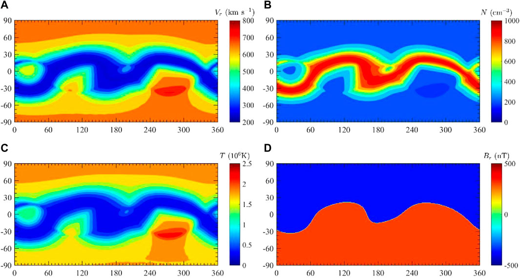
FIGURE 2. Maps of solar wind parameters at the lower boundary of 0.1 au for CR 2053. (A–D) The panels show the radial velocity Vr (km/s), number density N (cm⁻³), temperature T (K), and radial magnetic field Br (nT) (Shen et al., 2018).

Gonzi et al. (2021) investigated the impact of inner heliospheric boundary conditions on solar wind predictions at Earth. The radial component B_r was computed using two methods, the PFSS model or the magnetofrictional (MF) model. The solar wind velocity was obtained from three different methods. The first was the WSA model in Equation 2 using V_min = 240 km/s, V_max = 675 km/s, a₁ = 2/9, a₂ = 2.8°, a₃ = 1.25, and a₄ = 3. The second was a modified DCHB model $V_r({\theta }_b)=V_{\text{min}}+(V_{\text{max}}-V_{\text{min}}){({\theta }_b\cdot \omega )}^{\delta }$, and the parameters were chosen by comparing model-predicted solar wind speed histograms at 1 au with observations V_min = 200 km/s, V_max = 700 km/s, ω = 7 radian, and δ = 1.25. The third was determined by the interplanetary scintillation solar wind data. The number density was determined from the interplanetary scintillation solar wind data or the assumptions of the constant momentum flux NV², $N=N_s{\left(\frac{V_s}{V_r}\right)}^2$. The temperature was set as $T=T_s\frac{N_s}{N}$. Specifically, V_s = 300 km/s, N_s = 500cm⁻³, and T_s = 500 kK in the slow stream. The results showed that the selection of the coronal magnetic field model had a significant impact on the model results, and IPS data had a high success rate in reproducing high-speed solar wind.

2.2 Boundary conditions based on the PFSS + SCS model

Detman et al. (2006, 2011) introduced a Hybrid Heliospheric Modeling System (HHMS) for background solar wind to aid in the operational forecasting of geomagnetic activity, where the lower boundary was also set at 0.1 au. The radial magnetic field was provided by the PFSS + SCS model. The principle in determining the solar wind speed at 0.1 au was similar to the WS model given by the equation

$V_r\left(f_s\right)=V_{\text{min}}+\left(V_{\text{max}}-V_{\text{min}}\right)/{\left(1+\frac{f_s}{f_0}\right)}^{V_{\text{xp}}},(8)$

where V_max and V_min were set at 700 and 200 km/s, respectively. The parameter V_xp = 1.5 determined the sharpness of the fast–slow transition in the relationship. The parameter f₀ scaled the parameter f_s, which was adjustable to match the observed solar wind speeds. The mass density $\rho =\frac{F_{\text{mass}}}{V_r}$ was determined by the assumption of an constant mass flux, F_mass was obtained by taking observed values of ρV_r at Earth and applying an r² scaling to 0.1 au. The temperature $T=\frac{p_{\text{total}}-\frac{{\mathbf{B}}^2}{8\pi }}{2\rho R_{\text{gas}}}$ was determined by an assumption of the uniform total pressure p_total on the source surface, and p_total was a free parameter that required tuning. Figure 3 shows the block diagram of the HHMS in Detman et al. (2006).

FIGURE 3

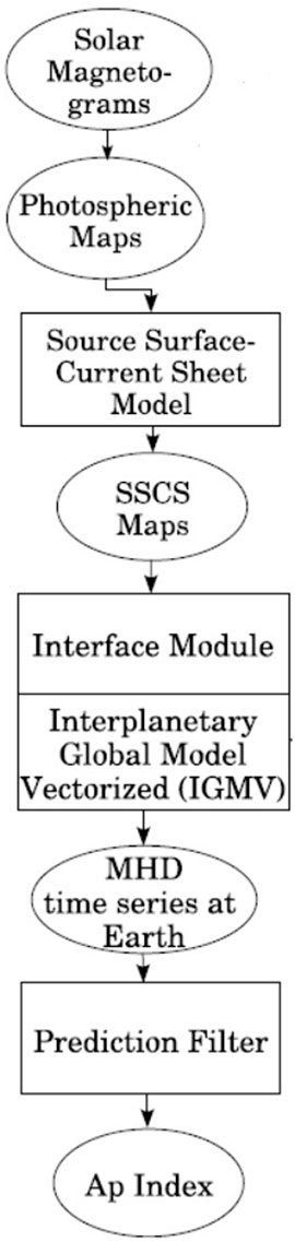
FIGURE 3. Block diagram of the HHMS (Detman et al., 2006).

Narechania et al. (2021) described a 3D MHD-based heliospheric model based on a semi-empirical data-driven approach. The inner boundary of the heliospheric model was set at 25 R_s, the magnetic field was derived by the PFSS + SCS model as in Detman et al. (2006), and the velocity was provided by Equation 2 with V_min = 250 km/s, V_max = 850 km/s, a₁ = 0.2, a₂ = 2.6°, a₃ = 1.25, and a₄ = 2.5. The remaining parameters were determined as in Shiota et al. (2014).

Pomoell and Poedts (2018) presented a new space weather forecasting-targeted inner EUropean Heliospheric FORecasting Information Asset (EUHFORIA) model. The plasma parameters at 0.1 au were obtained by using the empirical solar wind model. The radial component B_r was computed as

$B_r=\mathrm{sgn}\left(B_{\text{corona}}\right)B_{\text{max}}\left(V_r/V_{\text{max}}\right),(9)$

where sgn (B_corona) is the sign of the magnetic field as given by the PFSS + SCS model. B_max = 300 nT. The boundary value for the solar wind velocity was calculated according to Equation 2 with V_min = 240 km/s, V_max = 675 km/s, a₁ = 2/9, a₂ = 0.02 rad, a₃ = 1.25, and a₄ = 3. A constant value of 50 km/s is subtracted from the solar wind velocity to avoid systematically overestimating the wind speed. The number density is given as follows:

$N=N_{\text{fsw}}{\left(V_{\text{max}}/V_r\right)}^2,(10)$

where N_fsw = 300cm⁻³ is the number density of the fast solar wind. The temperature is given as $T=T_{\text{fsw}}{({\rho }_{\text{fsw}}/\rho )}^2$ with T_fsw = 0.8 MK. Figure 4 shows the sequence of steps that provides the boundary conditions for the heliospheric MHD model (Pomoell and Poedts, 2018).

FIGURE 4

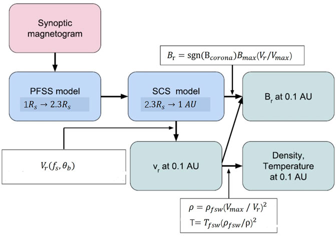
FIGURE 4. Sequence of steps that provide the boundary conditions for the heliospheric MHD model (Pomoell and Poedts, 2018).

2.3 Boundary conditions based on the CSSS model

The inner heliospheric solar wind was simulated from 21.5 R_s to 1 au with the MHD code CRONOS in Wiengarten et al. (2013) and Wiengarten et al. (2014). In Wiengarten et al. (2013), the CSSS model was used to obtain B_r at 21.5 R_s. The magnetic flux at the solar surface was obtained by the solar surface flux transport (SFT) model, which was then extrapolated to 10 solar radii by the CSSS model with R_CS = 1.55R_s and R_SS = 10R_s. Then, the radial magnetic field at the source surface was scaled to the lower boundary at 21.5 R_s by using the scale factor r⁻². In Wiengarten et al. (2014), the magnetic field at 0.1 au was derived by the PFSS + SCS model as in Detman et al. (2006). A Finite Difference Iterative Poisson Solver (FDIPS) was used to obtain the PFSS solution to avoid the numerical artifacts generated by the usual spherical harmonics expansion of the coronal potential field. At 0.1 au, the radial magnetic field was given a value of 300 nT, while keeping the orientation derived by the PFSS + SCS model. The radial velocity at 0.1 au was obtained with different forms for Wiengarten et al. (2013) and Wiengarten et al. (2014). Wiengarten et al. (2013) used $V_r=V_{\min }+\frac{V_{\text{del}}}{f_s^{V_{\text{xp}}}}+{\alpha }_1\cdot (\frac{{\theta }_b}{f_s^{V_{\text{xp}}/2}}-{\alpha }_2)$, where V_min = 154 km/s, V_del = 300 km/s, V_xp = 3, α₁ = 7.4 km/s, and α₂ = 3.5. The velocity V_r in Wiengarten et al. (2014) was calculated according to Equation 2 with V_min = 200 km/s, V_max = 675 km/s, a₁ = 2/9, a₂ ∈ (2.8°, 3.2°), a₃ = 2, and a₄ = 3. The remaining MHD quantities at the inner boundary were all similar to that described in Detman et al. (2006).

Li et al. (2020) simulated the interplanetary B_z using a data-driven heliospheric solar wind model. Following Merkin et al. (2016), the time-dependent boundary conditions were also used in their study. The radial component B_r at the inner boundary was derived from the CSSS model with R_CS = 2.5R_s and R_SS = 15R_s. The value of B_r given by the CSSS model was scaled by a factor b_up = Φ_OB/Φ_CSSS to provide enough magnetic flux at the inner boundary, where Φ_CSSS was the magnetic flux from the original CSSS solution and ${\mathrm{\Phi }}_{OB}=4\pi r_{\mathit{1au}}^2\mathrm{m}\mathrm{e}\mathrm{a}\mathrm{n}(B^{1\text{\hspace{0.17em}au}})/\sqrt{2}$ was the observed average magnetic flux at 1 au derived from OMNI data. The WSA model (Equation 2) was used to determine the solar wind velocity with V_min = 240 km/s, V_max = 560 km/s, a₁ = 2/9, a₂ = 2°, a₃ = 1, and a₄ = 3. As in Detman et al. (2006), the density was obtained by an assumption of a constant mass flux. The distribution of temperature at the heliobase was similar to that used in Shen et al. (2018) and Wang et al. (2020).

2.4 Boundary conditions based on in situ measurements

Biondo et al. (2021) described a new approach to determine the plasma parameters at the inner boundary of 0.1 au. This scheme applied a back reconstruction technique to remap the in situ measurements acquired at 1 au into the inner heliosphere. The observation data at 1 au were thought as a ring of L cells.

$\left[{\varphi }_i\left(rad\right),N_i\left(c{m}^{-3}\right),V_{r,i}\left(km/s\right),B_{r,i}\left(nT\right),B_{\varphi ,i}\left(nT\right)\right].(11)$

The Parker Spiral can be used to obtain their respective cells of origin $(0.1au;{\varphi }_i^{\prime })$.

${\varphi }_i^{\prime }={\varphi }_i+\frac{{\mathrm{\Omega }}_s}{v_{r,i}}\left(1au-0.1au\right).(12)$

The radial speed and numerical densities at 0.1 au can be obtained as follows:

$V_{r,i}^{\prime }=V_{r,i},$

$V_{\theta ,i}^{\prime }=0,$

$V_{\varphi ,i}^{\prime }=-{\mathrm{\Omega }}_s,r$

$N_i^{\prime }=N_i{\left(\frac{1au}{0.1au}\right)}^2.$

The treatment of the magnetic field was similar.

$B_{r,i}^{\prime }=B_{r,i}{\left(\frac{1au}{0.1au}\right)}^2,$

$B_{\theta ,i}^{\prime }=0,$

$B_{\varphi ,i}^{\prime }=B_{\varphi ,i}\left(\frac{1au}{0.1au}\right)+B_{r,i}\frac{{\mathrm{\Omega }}_s}{V_{r,i}}\left[\left(1au-R_{ss}\right)-\left(0.1au-R_{ss}\right){\left(\frac{0.1au}{1au}\right)}^2\right].$

This method could generate an interplanetary spiral reconstruction well with observations, and additionally, many small-scale features were also generated. Figure 5 presents the steps involved in RIMAP for the reconstruction of heliospheric plasma conditions (Biondo et al., 2021).

FIGURE 5

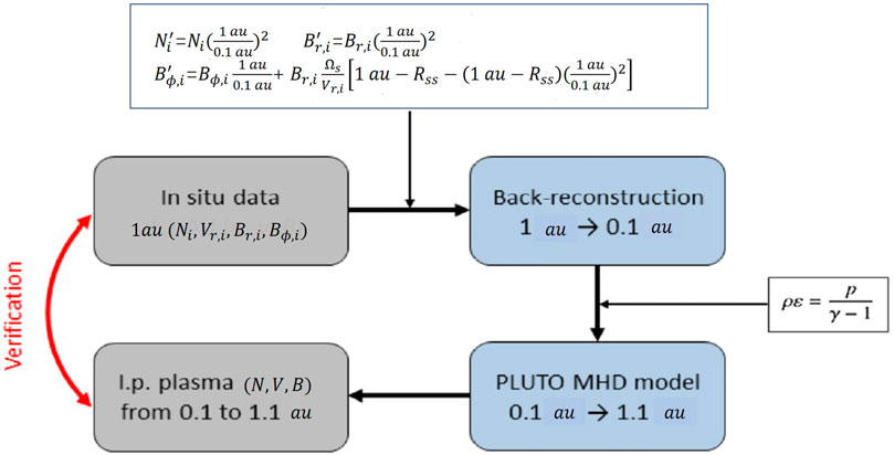
FIGURE 5. Schematic of the steps involved in RIMAP for the reconstruction of heliospheric plasma conditions starting from in situ measurements (Biondo et al., 2021).

2.5 Numerical simulation of solar wind with the Heliospheric Upwind eXtrapolation model

To provide a computationally efficient solution, the Heliospheric Upwind eXtrapolation (HUX) model (Riley and Lionello, 2011) was widely used to extrapolate velocity from near the Sun to 1 au without providing physical insight. The HUX model was essentially a 1D extrapolation with velocity in a radial direction.

$V_{r+1,\varphi }=V_{r,\varphi }+\frac{\mathrm{\Delta }r{\mathrm{\Omega }}_s}{V_{r,\varphi }}\left(\frac{V_{r+1,\varphi }-V_{r,\varphi }}{\mathrm{\Delta }\varphi }\right),(13)$

with Δr and Δϕ representing the grid spacing in radial and longitude directions, respectively. A comparative study of extrapolation models and empirical relations in forecasting solar wind was made in Kumar et al. (2020). The PFSS + SCS model was used to extrapolate magnetic fields. The velocity was obtained using the WS model or the WSA model. Then, the HUX model and a physics-based model PLUTO (Mignone et al., 2007) were used to extrapolate these velocities into the inner heliosphere zone, and the different magnetic field extrapolation models combined with velocity formulations were compared to predict the solar wind properties at L1. Figure 6 shows the sequence of steps used for each of these models.

FIGURE 6

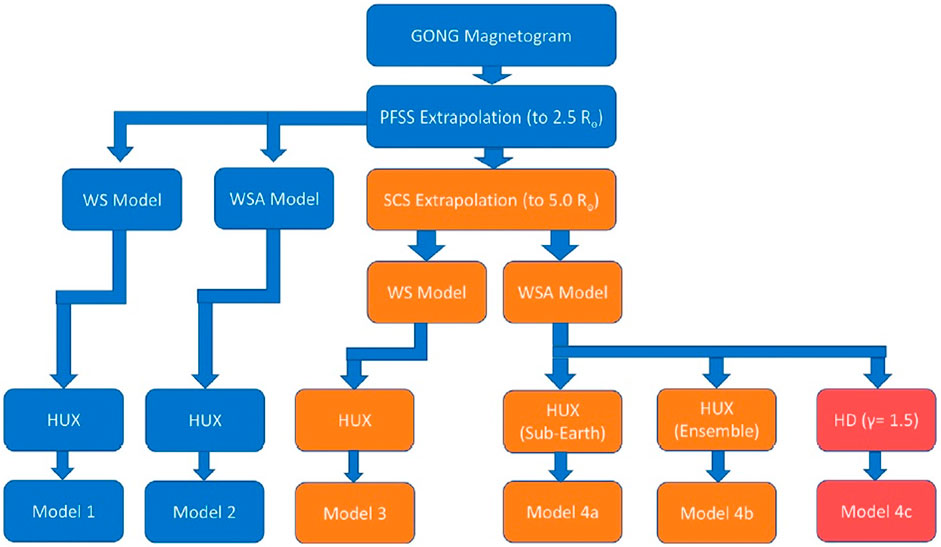
FIGURE 6. Flowchart of the models utilized in the work (Kumar et al., 2020).

They showed that the WSA model captures the contrast between the slow and fast solar wind better than the WS model. Additionally, the PFSS + SCS magnetic field extrapolation model combined with the WSA model had the best performance in all the cases.

Mayank et al. (2022) used a physics-based inner heliospheric model to forecast the ambient solar wind from 0.1 au to 2.1 au. The three-dimensional MHD equations were solved using the PLUTO code. The properties in the inner heliospheric model were derived from the PFSS + SCS model in combination with the WSA model (Equation 2). Additionally, the HUX algorithm was used to find the optimal set of values of independent parameters in the WSA model. The following parameters were chosen: V_min = 250 km/s, V_max = 650 km/s, a₁ = 2/9, a₂ = median of θ_bE, a₃ = 1.25, and a₄ = 3. θ_bE was calculated on the field lines that reached the location of Earth. Then, the WSA speed profile was rotated in the longitudinal direction by angle κ to account for solar rotation.

$\kappa =5+\left(\frac{2\pi }{{\mathrm{\Omega }}_s}\right)\left(\frac{21.5R_s}{{\left(V_r\right)}_{\text{min}}}\right).(14)$

Ω_s ranged from 27.21 to 27.34 days, depending on the location of Earth in its orbit. The radial component B_r and plasma number density were similar to those used by Pomoell and Poedts (2018). The plasma thermal pressure was chosen to be constant on the boundary and equal to p = 6.6 nPa. Figure 7 presents the process flow diagram of the proposed solar wind model showing the range of numerical models involved in the inner heliospheric model.

FIGURE 7

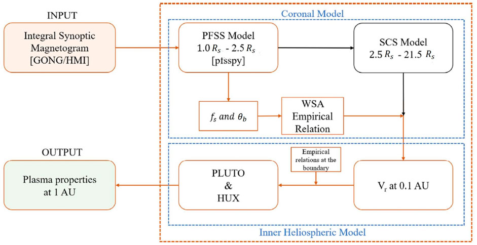
FIGURE 7. Process flow diagram of the proposed solar wind model showing the range of numerical models involved in the inner heliospheric model (Mayank et al., 2022).

The time-dependent form of the HUX model, which was referred to the HUXt model, was used to give solar wind velocity at Earth in Owens et al. (2020) and Bunting and Morgan (2022). Owens et al. (2020) set the inner boundary at 30 R_s, and the computed V_r at 30 R_s from the Magnetohydrodynamics Algorithm outside a Sphere (MAS) coronal model serves as the input to HUXt. They suggested that HUXt can act as a surrogate for full three-dimensional MHD models when very large ensembles are required. In Bunting and Morgan (2022), the inner boundary condition of the HUXt model was based on the coronal plasma density gained from coronagraph observations. The solar wind velocity was obtained using a simple linear relationship as follows:

$V=V_{\text{max}}-\left[\left(\frac{N-N_{\text{min}}}{N_{\text{max}}-N_{\text{min}}}\right)\left(V_{\text{max}}-V_{\text{min}}\right)\right],(15)$

where N_max and N_min are the maximum and minimum densities in the equatorial plane, respectively. The ambient solar wind velocity at Earth was obtained by using the HUXt model. Compared to an HUXt model with a traditional MAS as the input, the results showed that the tomography/HUXt model can predict solar wind velocity much better.

Overall, various inner boundary conditions have been developed in recent years, which provide important input conditions for space weather prediction. Table 1 summarizes the various methods to set the solar wind parameters at a lower boundary. The MHD model and the HUX model have been widely used for numerical simulation of solar wind. The HUX model can act as a surrogate for full three-dimensional MHD models when very large ensembles are required. However, it can only be used to obtain the velocity in the interplanetary space. Thus, the MHD model is necessary when we want to get other parameters, such as magnetic field, temperature, and density. For MHD simulation, these variables are all needed to be determined at the lower boundary initially. The magnetic field and velocity distribution are important because temperature and density are always determined from them. To calculate the magnetic field distribution, PFSS + SCS may be a better choice because the magnetic fields derived from the PFSS model have no thin HCS or Parker spiral in the interplanetary space. To better reflect the latitude-invariant nature of B_r, the CSSS model can be used. For calculating velocity distribution, the WSA model is better than the WS model in capturing the contrast between the slow and fast solar wind. The IPS observation has also been used to obtain velocity distribution, and the results show that IPS data has high success rate in detecting high-speed solar wind and the space weather prediction can be enhanced by the combination of MHD simulation and the IPS data.

TABLE 1

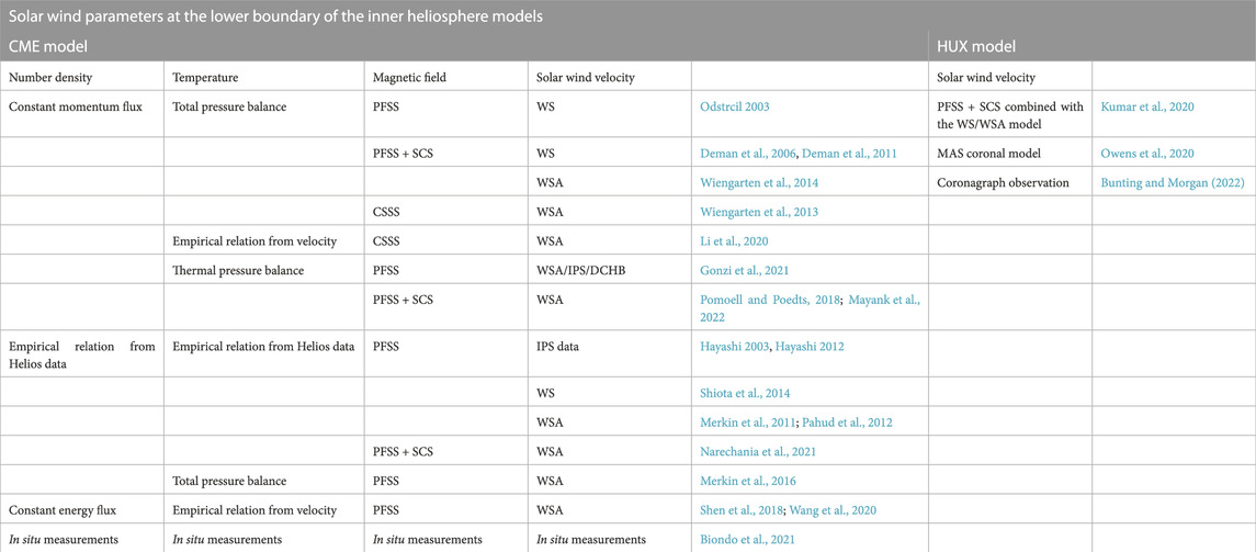
TABLE 1. Various methods used to set the solar wind parameters at the lower boundary.

It can be seen that the distribution of the inner boundary is fixed in many studies, the numerical processing on this fixed boundary is simple, and the steady-state solar wind can well represent the background conditions of the short-term transient phenomena using this fixed boundary. Since some studies used time-dependent boundary (Hayashi, 2012; Merkin et al., 2016; Li et al., 2020), it is expected that time-dependent boundary conditions can simulate the inner heliosphere more accurately and in real time. Fixed boundary conditions can accommodate observational data made in only one CR period. However, time-dependent boundary conditions can determine the MHD state of the solar wind at distant regions from the Sun, which are determined in a longer time period than one CR. Also, the heliospheric consequences of time-dependent conditions can be explored, that is, what kind of plasma and magnetic field structures are created due to the changing boundaries of coronal holes. Merkin et al. (2016) showed that time-dependent boundary conditions can reproduce the gross-scale structure of the heliosphere with higher fidelity, and provide important insights to interpret data on smaller spatial and faster time scales (e.g., 1 day). Thus, the time-dependent boundary condition is a promising direction of research both for space weather applications and fundamental physics of the heliosphere. For the time-dependent boundary, how to maintain the divergence-free condition is one difficulty. Since the time-dependent radial magnetic field $\frac{\partial B_r}{\partial t}$ is always obtained by observations, we need to derive an electric field tangential to the inner boundary spherical surface that would evolve the radial magnetic field. To do that, the Helmholtz theorem is applied on a sphere and the tangential electric field is expressed as the sum of the curl and the gradient of scalar potentials.

${\mathbf{E}}_t={\nabla }_t\times \psi \mathbf{r}+{\nabla }_t\mathrm{\Phi }.(16)$

Here, ψ is determined by solving the Poisson equation following Faraday’s law.

${\nabla }_t^2\psi =\frac{\partial B_r}{\partial t}.(17)$

Because there is no available information to determine Φ, Φ is always set to 0. Then, the transverse components of the magnetic field in the corotational frame can be calculated as follows:

$B_{\varphi }=B_r\frac{V_{\varphi }}{V_r}+\frac{E_{\theta }}{V_r},(18)$

$B_{\theta }=-\frac{E_{\varphi }}{V_r}.(19)$

3 Numerical simulation of the coronal mass ejection in the inner heliosphere

CMEs are giant clouds of magnetized plasma erupting from the Sun. When CMEs propagate through the corona and the interplanetary space, they interact with the solar wind plasma or other ICMEs and undergo changes. At larger heliocentric distances, CMEs are known to exhibit rotations and deflections, which can play a crucial role in their geomagnetic impact (Maharana et al., 2022). MHD simulations are often used for CME modeling purposes. There are two categories of MHD simulation models, one is anchored to the low corona and the other is fully embedded into the middle or upper corona. The first category is built through a large number of observations and enables the incorporation of more detailed physics, but the total computation time is much larger. On the other hand, the second category is suitable for space-weather forecasts because of the inexpensive computational cost and relative simplicity of implementation. Also, with the launch PSP and SO, the ICME will be constrained by more observations. In the past decades, many different models have been developed to simulate CME propagation in the heliosphere, such as ENLIL (Odstrcil, 2003), EUHFORIA (Pomoell and Poedts, 2018), SUSANOO-CME (Shiota and Kataoka, 2016), and MS-FLUKSS (Singh et al., 2020). In these models, CMEs are inserted at 0.1 au and evolved self-consistently by solving the MHD equations and a suitable CME initialization model is necessary. In this section, we focus on the initial CME parameters that need to be determined and extrapolated to the lower boundary.

The initial CME parameters rely heavily on CME reconstruction methods. The cone model (Zhao et al., 2002; Xie et al., 2004; Michaek, 2006) and the graduated cylindrical shell (GCS) model (Thernisien et al., 2006, 2009; Thernisien, 2011) are widely used to estimate the CME kinematic and geometric parameters in the past years. The cone model represents CME as a hydrodynamic pulse with a constant angular width, propagation direction, and speed. The angular width and source position of the CME are obtained by matching the modeled halos with the observed halos. The radial velocity and acceleration of the CME are determined by a series of times and radial distances. Figure 8 shows the cone model topology and relationship between the heliocentric coordinate system and the cone coordinate system (Michaek, 2006). The heliocentric coordinate system is defined such that x_h points to Earth, z_h points north, and y_h, z_h defines the sky plane. The cone coordinate system has the origin at the apex of the cone, z_c is the cone axis, and x_c, y_c defines the plane parallel to the base of the cone. The geometry of the cone can be determined by heliographic longitude ϕ, latitude θ, and angular width ω.For the GCS model, the CME is described as a flux-rope-like structure that expands in a self-similar fashion. The three-dimensional shape of the CME consists of two legs and a curved front. Figure 9 shows a face-on schematic of the GCS model (Thernisien et al., 2009) and schematic of the detailed geometric parameter (Thernisien, 2011). The dashed–dotted line shows the axis of the model, and the solid line the represents of the shell where the density is placed. The cross section of the model is a group of circular annuli with a gradually varying radii r₁ = κr, where r is the distance from a point on the shell to the center of the Sun and κ is a constant depending on the studied event. The angle between the axes of two conical legs is 2ω, and the height of the cone is h. The geometry of the shell can be completely defined with these three parameters. In the following section, lower boundary conditions in the existing inner heliospheric models are introduced in detail.

FIGURE 8

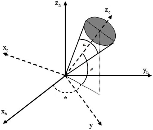
FIGURE 8. Cone model topology and relationship between the heliocentric coordinate system and the cone coordinate system (Michaek, 2006).

FIGURE 9

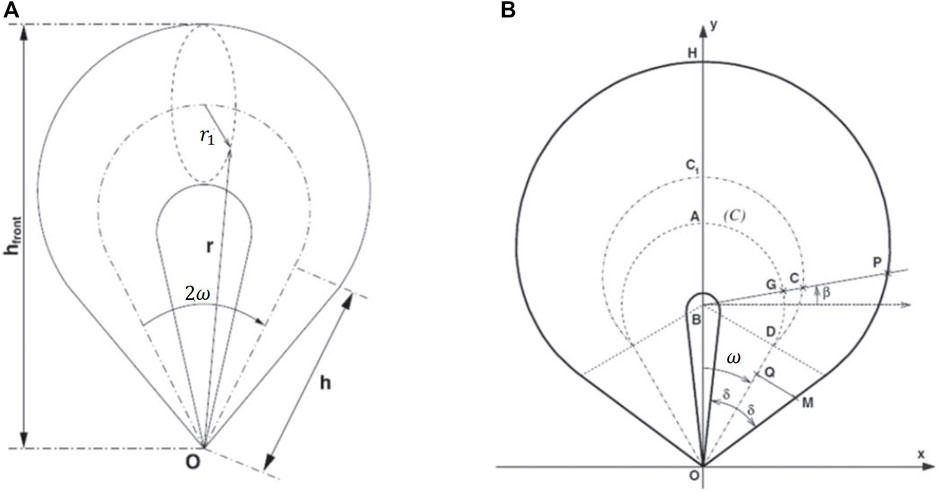
FIGURE 9. (A) Face-on schematic of the graduated cylindrical shell model (Thernisien et al., 2009), (B) Schematic of the detailed geometric parameter (Thernisien, 2011).

3.1 Numerical simulation of coronal mass ejection with hydrodynamic plasma cloud

Based on the cone model, the ENLIL model was used to simulate transient heliosphere disturbances (Odstrcil, 2003; Odstrcil et al., 2004; Odstrcil, 2005). A CME was simulated by launching a time-dependent hydrodynamic plasma cloud through the inner boundary of the heliospheric. The cone model was used to describe the location, speed, and angular width of the CME. The CME disturbance had uniform velocity, density, and temperature. The CME’s density (temperature) was taken to be four times larger than (equal to) the mean values in the fast stream. With the simple geometry, the ENLIL model had been successfully used to study the global evolution of CMEs in the heliosphere and predicted the CME arrival times at Earth. Figure 10 presents the distribution of solar wind parameters with the introduction of the input pulse on 12 May 1997 at 1800 UT (Odstrcil, 2005).

With the development of the EUHFORIA heliospheric model (Pomoell and Poedts, 2018), a new CME propagation model simulation was performed. The cone CME model was used to determine the CME angular width, propagation direction, and speed. Then, the CME was introduced to the inner radial boundary at 0.1 au as a time-dependent boundary condition. Specifically, the velocity, density, and temperature for solar wind values were replaced by constant values at R_gb = 0.1 au.

${\left(\theta -{\theta }_{\text{CME}}\right)}^2+{\left(\varphi -{\varphi }_{\text{CME}}\right)}^2<\alpha {\left(t\right)}^2,$

where the width as a function of time is

$\alpha \left(t\right)=\frac{{\omega }_{\text{CME}}}{2}\text{sin}\left[\frac{\pi }{2}\left(t-t_{\text{onset}}\right)/t_{\text{half}}\right],$

where t_half = R_gb tan (ω_CME/2)/v_CME, θ_CME, and ϕ_CME were the co-latitude and longitude of the propagation direction of the CME center, ω_CME was the angular width of the CME, and v_CME was the velocity of the CME. These parameters were provided by the cone model. For simplicity, the density and temperature of the modeled CMEs were taken to be density ρ_CME = 10⁻¹⁸kgm⁻³ and temperature T_CME = 0.8 MK, respectively. Scolini et al. (2018) used the EUHFORIA heliospheric model to test the effect of different CME shapes on simulation outputs, such as CME radius, the CME cross-section, and velocity initialization at the inner boundary. They showed that these geometrical parameters particularly affect predictions at locations hit by the CME, and the definition of the CME radius was the parameter having the greatest impact on simulation outputs. Verbeke et al. (2022) presented a new inner heliospheric model, ICARUS, for the simulation of the propagation and evolution of superposed CMEs. The cone CME model described in Scolini et al. (2018) was employed. For both scientific and forecasting purposes, the authors showed that the properties of radial grid stretching and solution adaptive mesh refinement were useful to save computational time.

3.2 Numerical simulation of coronal mass ejection with the flux-rope model

The geoeffectiveness of a CME is largely due to its magnetic field. If the CME contains a positive Bz component, it will be favorable for magnetic reconnection with Earth’s magnetosphere and results in a strong geomagnetic storms. The model described so far has not yet predicted the magnetic field structure of CMEs arriving at Earth. In order to overcome the limitations of the cone model, recent work has focused on modeling the CME using more realistic flux-rope models, such as spheromaks or toroidal-like structures.

The SUSANOO-CME model, developed by Shiota and Kataoka (2016), was used to simulate the interplanetary propagation of multiple CMEs with an internal magnetic flux-rope structure. The CME passed through the inner boundary at 30 R_s as the time evolution of the MHD variables. They adopted a spheromak-type magnetic flux rope, and radial compression was adopted for the flux rope to make the CME pass quickly. First, the CME model was defined as a simple linear force-free spheromak model near the Sun.

${\tilde{B}}_{\tilde{r}}\left(\tilde{r},\tilde{\theta },\tilde{\varphi }\right)=\left(2B_0/\alpha \tilde{r}\right)j_1\left(\alpha \tilde{r}\right)\text{cos}\tilde{\theta },$

${\tilde{B}}_{\tilde{\theta }}\left(\tilde{r},\tilde{\theta },\tilde{\varphi }\right)=-B_0\left[\frac{j_1\left(\alpha \tilde{r}\right)}{\alpha \tilde{r}}+j_1^{\prime }\left(\alpha \tilde{r}\right)\right]\text{sin}\tilde{\theta },$

${\tilde{B}}_{\tilde{\varphi }}\left(\tilde{r},\tilde{\theta },\tilde{\varphi }\right)=H\cdot B_0{j}_1\left(\alpha \tilde{r}\right)\text{sin}\tilde{\theta },$

where j₁ and j₀ are the first-order and zero-order spherical Bessel function, respectively. The CME was defined in local spherical coordinates $(\tilde{r},\tilde{\theta },\tilde{\varphi })$, the center of the CME was chosen to be the origin. Then, the CME model was shifted outward in the radial direction from the Sun to the inner boundary. The spherical cut $R_{\text{cut}}^{\prime }$ of the shifted magnetic configuration moved across the computational boundary as

$R_{\text{cut}}^{\prime }\left(t\right)=R_{\text{cut}}^{\prime }\left(t_0\right)-v_{\text{CME}}\left(t-t_0\right),$

where $R_{\text{cut}}^{\prime }(t_0)=30R_s$ defines the nose of the deformed spheromak. $t_0=t_{\text{onset}}+\frac{(30R_s-r_{\text{mc}})}{v_{\text{CME}}}$ is the start time when the CME appeared at the inner boundary. Finally, at the inner boundary, the magnetic field is given as

$B^{\prime }\left(30,\tilde{\theta },\tilde{\varphi }\right)=B^{\prime }\left(R_{\text{cut}}^{\prime }\left(t\right),\tilde{\theta },\tilde{\varphi }\right)=\tilde{B}\left(R_{\text{cut}}^{\prime }\left(t\right)-a,\tilde{\theta },\tilde{\varphi }\right),$

where a = 30R_s − r₀ − r_mc is the radial shift. The CME radius was r_mc = 1R_s ⋅ sin ω/2, and r₀ = 1R_s + r_mc was the distance between the central position of the spheromak and the heliospheric center. The model had 10 free parameters. t_onset was the onset time and v_CME was the propagation speed, which can be found from the LASCO CME catalog; λ_s and ϕ_s were heliographic latitude and longitude, respectively, which came from the flare list in National Geophysical Data Center (NGDC, https://www.ngdc.noaa.gov/stp/spaceweather.html); τ was the tilt angle of the spheromak (±90° with Hale–Nicholson law), χ was the inclination angle of the spheromak, H was the chirality of helicity in the spheromak (1, set −1 if opposite to the Bothmer–Schwenn rule), Φ_mag was the magnetic flux within CME, and w = 60° was the angular width of CME. The density inside the CME was in proportion to the magnetic field strength. The CME pressure was assumed to be a constant, which was defined as $\rho {(v_{\text{CME}}-v_{\text{SW}})}^2/2$. Because of the constant pressure and high density, the temperature was the lowest at the center of the flux rope.

Liu et al. (2019) used a three-dimensional flux-rope CME initialization model based on the GCS model to simulate the propagation and deflection of a CME from 21.5 R_s to 244 R_s. The Lundquist force-free CME model in a cylindrical geometry (r, ϕ, z) was used.

$B_r=0,$

$B_{\varphi }=H{B}_0{j}_1\left(\alpha \tilde{r}\right),$

$B_z=B_0{j}_1\left(\alpha \tilde{r}\right).$

The axial component of the magnetic field was assumed to be zero at the edge of the flux rope; thus, they could get

$\alpha R=2.405,$

where R stands for the radius of the cylindrical shell, which was obtained from the GCS model. The maximum of magnetic field B₀ is defined as

$B_0=\sqrt{\frac{2.405H_m}{4\pi LRj}},$

with $j={\int }_0^R{j}_1^2(\alpha \tilde{r})dr$, H_m is the magnetic helicity of the Lundquist flux rope and L = 2ω(H_front − R_front) is the flux-rope length, and H_front and R_front are the maximum height and maximum radius of the front, respectively, that were obtained from the GCS model. The initial density, velocity, and temperature at point P in the CME are given as follows:

${\rho }_{\text{CME}}={\rho }_{\text{max}}\left(1-\frac{d^2}{{\left(2r\right)}^2}\right),$

$v_{\text{CME}}=v_{\text{max}}\left(1-\frac{d^2}{{\left(2r\right)}^2}\right),$

$T_{\text{CME}}=T_{\text{max}}\left(1-\frac{d^2}{{\left(2r\right)}^2}\right).$

Within the GCS model, r represents the radius of the cross section and d stands for distance from point P to the center point at the front part, while defined as the distance from point P to the inner side of the cone in the cross-section plane. Table 2 shows the initial CME parameters (Liu et al., 2019).

FIGURE 10

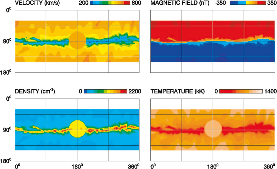
FIGURE 10. Distribution of solar wind parameters with the introduction of the input pulse on 12 May 1997 at 1800 UT (Odstrcil, 2005).

TABLE 2

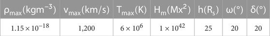
TABLE 2. Initial parameters of the CME (Liu et al., 2019).

Shen et al. (2021) made a numerical research on how the initial CME parameters can affect simulation results. They found that the initial density and geometric size of the CME both had an effect on its arrival time at Earth. The initial magnetic field had a large effect on the CME’s geomagnetic effect. All of these results confirmed that the initial geometric and physical parameters had an important role on space-weather research and forecasts.

The EUHFORIA CME model in Pomoell and Poedts (2018) and Scolini et al. (2018) did not contain an intrinsic magnetic field and was injected at the inner radial boundary with the enhancement of velocity, density, and pressure. Verbeke et al. (2019) introduced a linear force-free spheromak (LFFS) solution to the EUHFORIA CME model. The CME was considered to be a sphere with a radius r_mc = 0.1au ⋅ sin ω/2. The CME latitude and longitude (θ_CME, ϕ_CME), angular width ω, and speed v_CME were the same as in Pomoell and Poedts (2018). Located at (0.1au − r_mc, θ_CME, ϕ_CME), the CME moved through the 0.1 au boundary with speed v_CME. A point at (0.1au, θ, ϕ) satisfied the following formula was inside the CME

${\left(x_{\text{CME}}-x_{\text{bound}}\right)}^2+{\left(y_{\text{CME}}-y_{\text{bound}}\right)}^2+{\left(z_{\text{CME}}-z_{\text{bound}}\right)}^2\le r_{mc},(20)$

where (x_CME; y_CME; z_CME) and (x_bound; y_bound; z_bound) were the coordinates of the CME center and the considered point on the boundary in Cartesian HEEQ coordinates, respectively. The magnetic field was defined in a local spherical coordinate system $(\tilde{r},\tilde{\theta },\tilde{\varphi })$ as in Shiota and Kataoka (2016), with the center of the spheromak as the origin. As in Pomoell and Poedts (2018), density ρ_CME = 10⁻¹⁸kgm⁻³ and temperature T_CME = 0.8 MK. The initial speed required for the spheromak CME model should reflect only the radial speed.

$v_{\text{rad}}=v_{\text{cme}}\cdot \left[1-\frac{1}{1+\frac{1}{2}\left(1+\text{cot}w\right)}\right].(21)$

The remaining magnetic input parameters required in the spheromak CME model were the flux-rope handedness, tilt, and the toroidal magnetic flux at 0.1 au. The total toroidal flux Φ was used to define the magnetic field strength B₀.

$\mathrm{\Phi }=\iint {\tilde{B}}_{\tilde{\varphi }}\tilde{r}d\tilde{r}d\tilde{\theta }=\frac{2B_0}{{\alpha }^2}\cdot \left[-\text{sin}\left(\alpha r_0\right)+{\int }_0^{\alpha r_0}\frac{\text{sin}t}{t}dt\right].(22)$

In that paper, a +1 handedness with a 90.0° tilt angle were selected to obtain a negative Bz magnetic field when the CME was arriving at Earth. Lastly, the total toroidal flux was set to be 10¹⁴ Wb to produce the best results they performed so far. Figure 11 shows the magnetic field lines depicting the structure of the LFFS CME model with a 90.0° tilt (Verbeke et al., 2019).

FIGURE 11

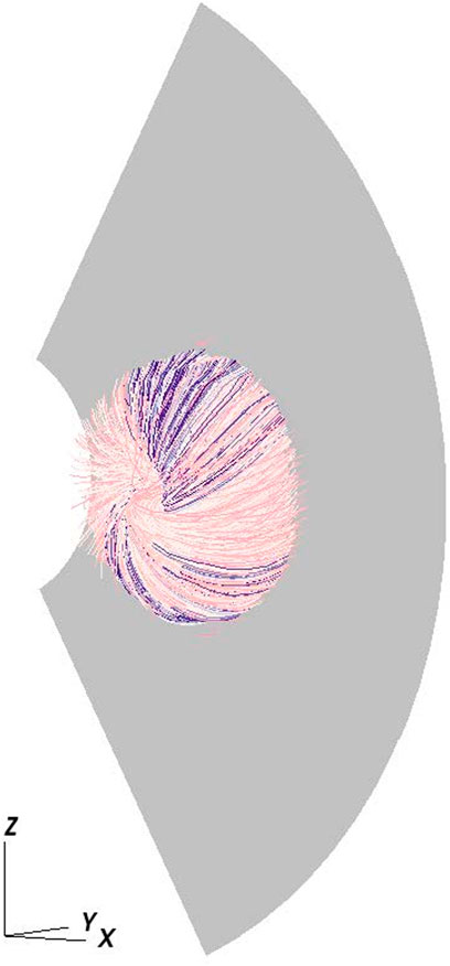
FIGURE 11. Magnetic field lines depicting the structure of the LFFS CME model with a 90.0° tilt (Verbeke et al., 2019).

Zhang et al. (2021) performed a numerical study of two injection methods for CME in the inner heliosphere, where CASE-1 CME was introduced into the inner boundary with a radial compression (Shiota and Kataoka, 2016) and CASE-2 CME was introduced into the inner boundary without a radial compression (Scolini et al., 2019; Scolini et al., 2020; Verbeke et al., 2019). The CME angular width was obtained by using the sky-plane-projected speed range (Gopalswamy et al., 2010). The CME mass density and temperature were set to be homogeneous as in Pomoell and Poedts (2018); Verbeke et al. (2019). The CME position, velocity, and magnetic input parameters were estimated from image modeling and geometric triangulation analysis following Liu et al. (2010). They found that CASE-2 CME overestimated the radial extension at 1 au and the modeled magnetic fields at 1 au were lower compared to CASE-1 CME. Figure 12 shows the three-dimensional view of the magnetic field for CASE-1 and CASE-2 at different times. The top row shows the three-dimensional view of the magnetic field at 0.4 h (left), 2.0 h (right) after the addition of the CME into the ambient solar wind for CASE-1, while the bottom row shows the magnetic field at 5 h (left), 15 h (right) after the addition of the CME into the ambient solar wind for CASE-2. Solid black lines display the magnetic field lines and the color code represents the magnetic field B in units of 10⁵ T. The blue sphere represents the 20 R_s (Zhang et al., 2021).

FIGURE 12

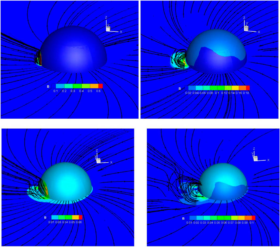
FIGURE 12. Three-dimensional view of the magnetic field for CASE-1 and CASE-2 at different times (Zhang et al., 2021).

Cone CMEs in Pomoell and Poedts (2018) were initialized using a set of seven input parameters during the CME insertion at the inner boundary of the heliospheric model. For example, the CME insertion time, speed v_CME, source (θ_CME, ϕ_CME), and half angular width ω/2 at 0.1 au were usually derived from cone model. In addition, the CME mass density and temperature were set to be homogeneous with density ρ_CME = 10⁻¹⁸kgm⁻³ and temperature T_CME = 0.8 MK. When simulated CMEs use the spheromak model as in Verbeke et al. (2019), three additional input parameters were needed: the helicity sign (chirality), the tilt, and the toroidal magnetic flux at 0.1 au. Since the spheromak CME in Verbeke et al. (2019) was initialized from observations partially, Scolini et al. (2019, 2020) aimed to constrain all the CME input parameters from remote-sensing observations. The CME geometric and kinematic parameters were derived using the GCS model: the CME direction, the height of the CME apex h_front, the tilt angle around the axis of symmetry γ (with respect to the solar equator), the half angle between the legs ω, and the half angle of the cone δ related to the “aspect ratio” κ by the relation κ = sin δ. The 3D speed at the CME apex was derived from the GCS model with a sequence of images.

$v_{\text{CME}}=\frac{d{h}_{\text{front}}}{dt}.$

Then, the radial and expansion contribution were obtained as follows:

$v_{\text{rad}}=\frac{1}{1+\kappa }\frac{d{h}_{\text{front}}}{dt},$

$v_{\text{exp}}=\frac{\kappa }{1+\kappa }\frac{d{h}_{\text{front}}}{dt}.$

The flux-rope handedness was determined from pre-eruption EUV sigmoids observations. The flux-rope tilt angle/orientation was inferred from the orientation of the source region polarity inversion line (PIL) and/or from the orientation of the post-eruption arcades (PEAs). The flux-rope toroidal magnetic flux was based on the reconnected flux, which was computed by the FRED method described by Gopalswamy et al. (2017). Using the PEA area, the FRED method computed the total (unsigned) magnetic flux from line-of-sight magnetic field data. Then, the reconnected flux ϕ_RC could be obtained as follows:

${\varphi }_{\text{RC}}=\frac{1}{2}{\int }_{\text{PEA}}|B_{\text{los}}|dA=\frac{1}{2}|B_{\text{los}}{|}_{\text{tot}}{A}_{\text{PEA}}.$

The axial field strength B₀ was estimated with the following formula:

$B_0=\frac{{\alpha }^3}{2\pi }\frac{{\varphi }_p\left(r_{\star }\right)r_{\star }}{\left(\text{sin}\left(\alpha r_{\star }\right)-\alpha r_{\star }\text{cos}\left(\alpha r_{\star }\right)\right)},$

where r_⋆ is the distance from the center of the spheromak, on the plane $\theta =\frac{\pi }{2}$, where the magnetic field becomes completely axial. ϕ_p (r_⋆) was the poloidal magnetic flux that is transferred from the reconnected flux.

Maharana et al. (2022) introduced a fully analytical “Flux Rope in 3D” (FRi3D) CME model to EUHFORIA (Pomoell and Poedts, 2018) to improve the modeling of CME flank encounters. The geometrical parameters for the FRi3D flux rope contained the half-width φ_hw in the azimuthal direction, the angular half-height φ_hh in the polar direction, the toroidal height R_t defined the heliocentric distance to the apex of the CME axis, a coefficient n defined the deformation at the CME front, pancaking φ_p meant the deformation due to radial expansion, and skew φ_s defined the deformation due to solar rotation. The geometrical parameters were obtained by using the forward modeling tool of FRi3D to remote multi-viewpoint observations. The Lundquist model in cylindrical geometry was used to get the magnetic field configuration of the CME. The magnetic field parameters, such as the tilt, the magnetic flux, the twist, the chirality, and the polarity, were obtained by fitting the FRi3D CME model to WIND spacecraft at 1 au (Isavnin, 2016). The FRi3D CME model was also filled with uniform density plasma with density ρ_CME = 10⁻¹⁷kgm⁻³ and temperature T_CME = 0.8 MK. Figure 13 shows a FRi3D flux rope emerging out of EUHFORIA’s inner heliospheric boundary at 0.1 au. The color of the field lines is based on the magnetic field strength. The field lines are twisted and deformed as per a particular CME geometry and have maximum strength close to the axis which reduces outward (typical Lundquist model characteristics) (Maharana et al., 2022).

FIGURE 13

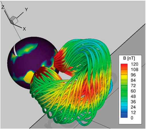
FIGURE 13. FRi3D flux rope emerging out of the EUHFORIA’s inner heliospheric boundary at 0.1 AU (Maharana et al., 2022).

Singh et al. (2020) applied a modified spheromak model for simulations of the CME in the inner heliosphere. The simulations were carried out using a MultiScale Fluid-Kinetic Simulation Suite (MS-FLUKSS) code. They introduced a modified spheromak flux rope into the solar wind, where the poloidal and toroidal fluxes were set up independently.

$\vec{b}=\frac{1}{r\text{sin}\theta }\left(\zeta \frac{1}{r}\frac{\partial A}{\partial \theta }\widehat{r}-\zeta \frac{\partial A}{\partial r}\widehat{\theta }+H{\alpha }_{0}A\widehat{\varphi }\right),$

$A=\frac{4\pi a_1}{{\alpha }_0^2}\left[\frac{r_0^2}{g\left({\alpha }_{0}r\right)}-r^2\right]{\text{sin}}^2\theta ,$

$g\left({\alpha }_{0}r\right)=\frac{\text{sin}\left({\alpha }_{0}r\right)}{{\alpha }_{0}r}-\text{cos}\left({\alpha }_{0}r\right),$

where α₀r_mc = 5.763,459. The origin of the spherical coordinate system was placed at the spheromak center. The flux-rope parameters were introduced into the solar wind as follows:

${\vec{b}}_{\mathit{final}}={\vec{b}}_{FR},$

${\rho }_{\mathit{final}}={\rho }_{FR}+{\rho }_{SW},$

$e_{\mathit{final}}=\xi e_{FR}+e_{SW},$

where ξ was related to plasma β as β ∼ (γ − 1) (ξ − 1) indicated that the magnetic pressure in the flux rope was larger than the pressure in the solar wind. The mass inside the spheromak was a constant with 1.65 × 10¹⁵ g. The thermal pressure was assumed to be proportional to the magnetic pressure. The poloidal flux and the toroidal flux were set to be 2 × 10²² Mx and 5 × 10²¹ Mx, respectively. A positive helicity sign was used. Figure 14 shows the magnetic field line configuration of the modified spheromak inserted at the inner boundary (Singh et al., 2020).

FIGURE 14

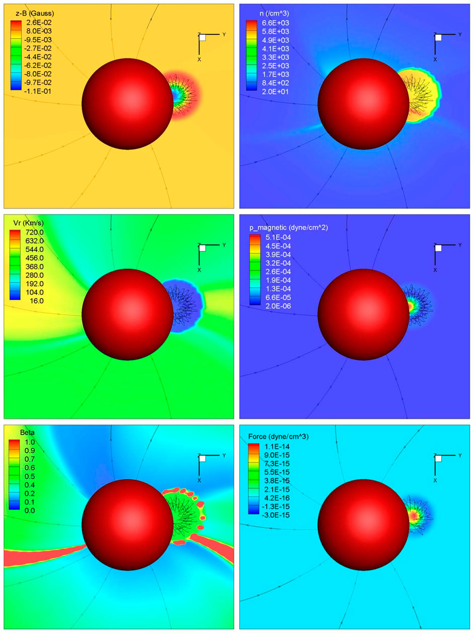
FIGURE 14. Magnetic field line configuration of the modified spheromak inserted at the inner boundary R = 0.1 AU, shown with the red sphere (Singh et al., 2020).

Table 3 summarizes the various methods to set the CME parameters at lower boundary. Since the ability of a CME to disturb the near-Earth space is largely due to its magnetic fields, the flux-rope model is widely used in recent years because of its internal magnetic fields structure. How to constrain the initial CME parameters by observations is one difficulty. The cone model and GCS model are widely used to estimate the CME kinematic and geometric parameters. The magnetic field parameters, such as handedness, tilt, and toroidal magnetic flux, are deduced from remote-sensing observations in Scolini et al. (2019, 2020). With the launch of the PSP and SO into the inner heliosphere, the ICME will be constrained by more observations.

TABLE 3

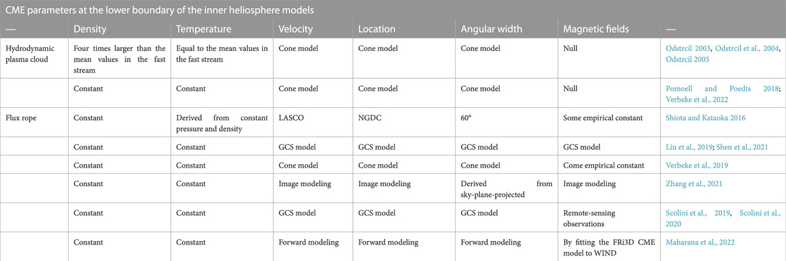
TABLE 3. Various methods to set the CME parameters at the lower boundary.

4 Conclusion and discussion

Overall, the three-dimensional MHD numerical model has become an important tool to report interplanetary solar wind and the CME. The MHD heliospheric model is relatively cheap in terms of calculation, and it takes tens of minutes to hours to simulate the CME propagation from the Sun to Earth. The operational space-weather forecast is usually generated by the heliospheric model. The resulting forecast errors are largely dependent on the uncertainty of the inner boundary conditions, rather than the heliospheric model.

For the solar wind simulation in the inner heliosphere, the solar wind density and temperature at the inner boundary are always derived as a function of the solar wind speed and magnetic field; thus, the speed and magnetic field can significantly affect the accuracy of the simulated results. The speed specified by the WSA formula given in Eq. 2 seems to be the most efficient formula. However, there are several free parameters in the WSA model, whose uncertainties may result in the deviations between the simulated results and observations. Thus, how to make parameter optimization is a major problem. The dynamic time warping (DTW) algorithm described in Bunting and Morgan (2022) can be used to derive the optimized values for the speed in the WSA formula. DTW algorithm is effective to quantify the agreement between two time series and has recently been used in a variety of fields such as economics, biology, and space weather. Here, DTW distance is used to measure the difference between the model and in situ solar wind velocities, and a smaller DTW distance means that the modeled data is in good agreement with the in situ data. The initial parameters of the WSA formula were adjusted to minimize the DTW distance, and then, we can obtain the optimized parameters in WSA formula. Also, the IPS observation is a good choice to obtain the velocity distribution, and the results show that IPS data have a high success rate in detecting high-speed solar wind and the space-weather prediction can be enhanced by the combination of MHD simulation and the IPS data. For the magnetic field at the inner boundary, the PFSS model is always used. However, the PFSS model underestimated the magnetic flux in the heliosphere. Shen et al. (2018) only kept the polarity of the magnetic field from the PFSS model and used the observational data at 1 au in the immediate past to limit the value of the magnetic field, and the results showed that the modeled magnetic field at 1 au agrees with the in situ observations much better. Additionally, the magnetic fields derived from the PFSS model have no thin HCS or Parker spiral in the interplanetary space; thus, the PFSS + SCS model may be a good choice.

For the CME simulation in the inner heliosphere, CMEs are always initialized by flux-rope models, such as spheromaks or toroidal-like structures, and the CMEs are introduced to the inner radial boundary as a time-dependent boundary. Scolini et al. (2019, 2020) suggested that the prediction of the CME arrival time at Earth was found to be highly dependent on the CME model and CME input parameters used. Thus, how to obtain the CME parameters at the inner boundary is important. At present, CME geometric and kinematic parameters, such as CME position, radius, and velocity, are always derived from the GCS model or the cone model. The density and temperature of the CMEs are assumed to be constant. To improve the prediction of the CME internal magnetic field at Earth, it is necessary to constrain the flux-rope magnetic parameters from the remote-sensing observations of the corona. Scolini et al. (2019, 2020) constrained flux-rope magnetic parameters from remote-sensing observations, and the results showed that the current model can improve the predictions of B_z up to 22–40 percentage points compared to a cone model.

At present, the numerical simulation in the inner heliosphere has a large dependence on the empirical model. How to use the observations to constrain the uncertainties in the empirical models is something we must consider in future. Maybe we can use the in situ data in the past CR to correct the uncertainties in the empirical models at the current CR, but this can only be applicable to the solar wind. With the multi-spacecraft observations in the future, such as SO and PSP, the detailed measurements of the inner heliosphere will be provided. All of these will provide us with more realistic inner boundary conditions, and we will have a deeper understanding of the triggering and propagation evolution of solar wind and disturbance.

Author contributions

XF designed the research. MZ and HL participated in data analyses and the writing of the manuscript. MX, FS, LY, XZ, YZ, and XL participated in data interpretation and discussion. All authors read and agreed to the published version of the manuscript.

Funding

The work was jointly supported by the National Natural Science Foundation of China (Grant Nos. 42030204 and 41874202), the National Key R&D Program of China (Grant No. 2022YFF0503900), the Shenzhen Natural Science Fund (the Stable Support Plan Program GXWD20220817152453003), and the Specialized Research Fund for State Key Laboratories.

Conflict of interest

The authors declare that the research was conducted in the absence of any commercial or financial relationships that could be construed as a potential conflict of interest.

Publisher’s note

All claims expressed in this article are solely those of the authors and do not necessarily represent those of their affiliated organizations, or those of the publisher, the editors, and the reviewers. Any product that may be evaluated in this article, or claim that may be made by its manufacturer, is not guaranteed or endorsed by the publisher.

References

Altschuler, M. D., and Newkirk, G. J. (1969). Magnetic fields and the structure of the solar corona. Sol. Phys. 9, 131–149. doi:10.1007/bf00145734

CrossRef Full Text | Google Scholar

Arge, C. N., Luhmann, J. G., Odstrcil, D., Schrijver, C. J., and Li, Y. (2004). Stream structure and coronal sources of the solar wind during the may 12th, 1997 cme. J. Atmos. Solar-Terrestrial Phys. 66, 1295–1309. doi:10.1016/j.jastp.2004.03.018

CrossRef Full Text | Google Scholar

Arge, C. N., and Pizzo, V. J. (2000). Improvement in the prediction of solar wind conditions using near-real time solar magnetic field updates. J. Geophys. Res. 105, 10465–10479. doi:10.1029/1999ja000262

CrossRef Full Text | Google Scholar

Biondo, R., Bemporad, A., Mignone, A., and Reale, F. (2021). Reconstruction of the parker spiral with the reverse in situ data and mhd approach-rimap. J. Space Weather Space Clim. 11, 7. doi:10.1051/swsc/2020072

CrossRef Full Text | Google Scholar

Bochsler, P., Balsiger, H., Gloeckler, G., Burgi, A., Fisk, L., Galvin, A., et al. (1995). The solar wind and suprathermal ion composition investigation on the wind spacecraft. Space Sci. Rev. 71, 79–124. doi:10.1007/bf00751327

CrossRef Full Text | Google Scholar

Bunting, K. A., and Morgan, H. (2022). An inner boundary condition for solar wind models based on coronal density. J. Space Weather Space Clim. 12, 30. doi:10.1051/swsc/2022026

CrossRef Full Text | Google Scholar

Chat, G. L., Issautier, K., and Meyer-Vernet, N. (2012). The solar wind energy flux. Sol. Phys. 279, 197–205. doi:10.1007/s11207-012-9967-y

CrossRef Full Text | Google Scholar

Detman, T., Smith, Z., Dryer, M., Fry, C. D., Arge, C. N., and Pizzo, V. (2006). A hybrid heliospheric modeling system: Background solar wind. J. Geophys. Res. 111, A07102. doi:10.1029/2005ja011430

CrossRef Full Text | Google Scholar

Detman, T. R., Intriligator, D. S., Dryer, M., Sun, W., Deehr, C. S., and Intriligator, J. (2011). The influence of pickup protons, from interstellar neutral hydrogen, on the propagation of interplanetary shocks from the halloween 2003 solar events to ACE and Ulysses: A 3-D MHD modeling study. J. Geophys. Res. 116. doi:10.1029/2010ja015803

CrossRef Full Text | Google Scholar

Elliott, H. A., McComas, D. J., Schwadron, N. A., Gosling, J. T., Skoug, R. M., Gloeckler, G., et al. (2005). An improved expected temperature formula for identifying interplanetary coronal mass ejections. J. Geophys. Res. Space Phys. 110, A04103. doi:10.1029/2004ja010794

CrossRef Full Text | Google Scholar

Feng, X. (2020). Magnetohydrodynamic modeling of the solar corona and heliosphere. Singapore: Springer. doi:10.1007/978-981-13-9081-4

CrossRef Full Text | Google Scholar

Feng, X. S., Zhang, M., and Zhou, Y. F. (2014). A new three-dimensional solar wind model in spherical coordinates with a six-component grid. Astrophysical J. Suppl. 214, 6. doi:10.1088/0067-0049/214/1/6

CrossRef Full Text | Google Scholar

Fox, N. J., Velli, M. C., Bale, S. D., Decker, R., Driesman, A., Howard, R. A., et al. (2016). The solar probe plus mission: Humanity’s first visit to our star. Space Sci. Rev. 204, 7–48. doi:10.1007/s11214-015-0211-6

CrossRef Full Text | Google Scholar

Gonzi, S., Weinzierl, M., Bocquet, F., Bisi, M. M., Odstrcil, D., Jackson, B. V., et al. (2021). Impact of inner heliospheric boundary conditions on solar wind predictions at Earth. Space Weather. 19, 13. doi:10.1029/2020sw002499

CrossRef Full Text | Google Scholar

Gopalswamy, N., Yashiro, S., Akiyama, S., and Xie, H. (2017). Estimation of reconnection flux using post-eruption arcades and its relevance to magnetic clouds at 1 au. Sol. Phys. 292, 65. doi:10.1007/s11207-017-1080-9

CrossRef Full Text | Google Scholar

Gopalswamy, N., Yashiro, S., Michalek, G., Xie, H., Makela, P., Vourlidas, A., et al. (2010). A catalog of halo coronal mass ejections from soho. Am. Geophys. Union 5, 7–16.

Google Scholar

Hayashi, K. (2012). An mhd simulation model of time-dependent co-rotating solar wind. J. Geophys. Res. 117, A08105. doi:10.1029/2011ja017490

CrossRef Full Text | Google Scholar

Hayashi, K. (2003). Mhd tomography using interplanetary scintillation measurement. J. Geophys. Res. Space Phys. 108, 1102. doi:10.1029/2002ja009567

CrossRef Full Text | Google Scholar

Howard, R., Moses, J., Vourlidas, A., Newmark, J., Socker, D., Plunkett, S., et al. (2008). Sun Earth connection coronal and heliospheric investigation (secchi). Space Sci. Rev. 136, 67–115. doi:10.1007/s11214-008-9341-4

CrossRef Full Text | Google Scholar

Isavnin, A. (2016). Fried: A novel three-dimensional model of coronal mass ejections. Astrophysical J. 833, 267. doi:10.3847/1538-4357/833/2/267

CrossRef Full Text | Google Scholar

Kaiser, M., Kucera, T., Davila, J., and St. Cyr, O. C. (2008). The STEREO mission: An introduction. Space Sci. Rev. 136, 5–16. doi:10.1007/s11214-007-9277-0

CrossRef Full Text | Google Scholar

Kilpua, E. K. J., Lugaz, N., Mays, M. L., and Temmer, M. (2019). Forecasting the structure and orientation of earthbound coronal mass ejections. Space Weather. 17, 498–526. doi:10.1029/2018sw001944

CrossRef Full Text | Google Scholar

Kumar, S., Paul, A., and Vaidya, B. (2020). A comparison study of extrapolation models and empirical relations in forecasting solar wind. Front. Astronomy Space Sci. 7, 572084. doi:10.3389/fspas.2020.572084

CrossRef Full Text | Google Scholar

Li, H., Feng, X., Zuo, P., and Wei, F. (2020). Simulation of the interplanetary B_z using a data-driven heliospheric solar wind model. Astrophysical J. 900, 76. doi:10.3847/1538-4357/aba61f

CrossRef Full Text | Google Scholar

Liu, Y., Shen, F., and Yang, Y. (2019). Numerical simulation on the propagation and deflectio n of fast coronal mass ejections (cmes) interacting with a corotating interaction region in interplanetary space. Astrophysical J. 887, 150. doi:10.3847/1538-4357/ab543e

CrossRef Full Text | Google Scholar

Liu, Y., Thernisien, A., Luhmann, J., Vourlidas, A., Davies, J., Lin, R., et al. (2010). Reconstructing coronal mass ejections with coordinated imaging and in situ observations: Global structure, kinematics, and implications for space weather forecasting. Astrophysical J. 722, 1762–1777. doi:10.1088/0004-637x/722/2/1762

CrossRef Full Text | Google Scholar

Lopez, R. E., and Freeman, J. W. (1986). Solar wind proton temperature-velocity relationship. J. Geophys. Res. Space Phys. 91, 1701–1705. doi:10.1029/ja091ia02p01701

CrossRef Full Text | Google Scholar

Mackay, D. H., and Yeates, A. R. (1999). The suns global photospheric and coronal magnetic fields: Observations and models. Living Rev. Sol. Phys. 9, 1–50. doi:10.12942/lrsp-2012-6

CrossRef Full Text | Google Scholar

Maharana, A., Isavnin, A., Scolini, C., Wijsen, N., Rodriguez, L., Mierla, M., et al. (2022). Implementation and validation of the FRi3d flux rope model in EUHFORIA. Adv. Space Res. 70, 1641–1662. doi:10.1016/j.asr.2022.05.056

CrossRef Full Text | Google Scholar

Mayank, P., Vaidya, B., and Chakrabarty, D. (2022). SWASTi-SW: Space weather adaptive simulation framework for solar wind and its relevance to the aditya-l1 mission. Astrophysical J. Suppl. Ser. 262, 23. doi:10.3847/1538-4365/ac8551

CrossRef Full Text | Google Scholar

Mcgregor, S. L., Hughes, W. J., Arge, C. N., Owens, M. J., and Odstrcil, D. (2011). The distribution of solar wind speeds during solar minimum: Calibration for numerical solar wind modeling constraints on the source of the slow solar wind. J. Geophys. Res. Space Phys. 116, A03101. doi:10.1029/2010ja015881

CrossRef Full Text | Google Scholar

Merkin, V. G., Lyon, J. G., Lario, D., Arge, C. N., and Henney, C. J. (2016). Time-dependent magnetohydrodynamic simulations of the inner heliosphere. J. Geophys. Res. Space Phys. 121, 2866–2890. doi:10.1002/2015ja022200

CrossRef Full Text | Google Scholar

Merkin, V. G., Lyon, J. G., Mcgregor, S. L., and Pahud, D. M. (2011). Disruption of a heliospheric current sheet fold. Geophys. Res. Lett. 38, L14107. doi:10.1029/2011gl047822

CrossRef Full Text | Google Scholar

Michaek, G. (2006). An asymmetric cone model for halo coronal mass ejections. Sol. Phys. 237, 101–118. doi:10.1007/s11207-006-0075-8

CrossRef Full Text | Google Scholar

Mignone, A., Bodo, G., Massaglia, S., Matsakos, T., Tesileanu, O., Zanni, C., et al. (2007). Pluto: A numerical code for computational astrophysics. Astrophysical J. Suppl. Ser. 170, 228–242. doi:10.1086/513316

CrossRef Full Text | Google Scholar

Müller, D., St Cyr, O. C., Zouganelis, I., Gilbert, H. R., Marsden, R., Nieves-Chinchilla, T., et al. (2020). The Solar Orbiter mission. Science overview. Astronomy Astrophysics 642, A1. doi:10.1051/0004-6361/202038467

CrossRef Full Text | Google Scholar

Nakamizo, A., Tanaka, T., Kubo, Y., Kamei, S., Shimazu, H., and Shinagawa, H. (2009). Development of the 3-D MHD model of the solar corona-solar wind combining system. J. Geophys. Res. 114, A07109. doi:10.1029/2008ja013844

CrossRef Full Text | Google Scholar

Narechania, N. M., Nikolic, L., Freret, L., Sterck, H. D., and Groth, C. (2021). An integrated data-driven solar wind-cme numerical framework for space weather forecasting. J. Space Weather Space Clim. 11, 8. doi:10.1051/swsc/2020068

CrossRef Full Text | Google Scholar

Odstrcil, D., And, P. R., and Zhao, X. P. (2004). Numerical simulation of the 12 may 1997 interplanetary cme event. J. Geophys. Res. Space Phys. 109, A02116. doi:10.1029/2003ja010135

CrossRef Full Text | Google Scholar

Odstrcil, D. (2005). Propagation of the 12 may 1997 interplanetary coronal mass ejection in evolving solar wind structures. J. Geophys. Res. 110, A02106. doi:10.1029/2004ja010745

CrossRef Full Text | Google Scholar

Odstrcil, D. (2003). Modeling 3-D solar wind structure. Adv. Space Res. 32, 497–506. doi:10.1016/s0273-1177(03)00332-6

CrossRef Full Text | Google Scholar

Owens, M., Lang, M., Barnard, L., Riley, P., Gonzi, S., Scott, C. J., et al. (2020). A computationally efficient, time-dependent model of the solar wind for use as a surrogate to three-dimensional numerical magnetohydrodynamic simulations. Sol. Phys. 295, 43. doi:10.1007/s11207-020-01605-3

CrossRef Full Text | Google Scholar

Owens, M. J., Spence, H. E., McGregor, S., Hughes, W. J., Quinn, J. M., Arge, C. N., et al. (2008). Metrics for solar wind prediction models: Comparison of empirical, hybrid, and physics-based schemes with 8 years of L1 observations. Space Weather. 6, S08001. doi:10.1029/2007sw000380

CrossRef Full Text | Google Scholar

Pahud, D. M., Merkin, V. G., Arge, C. N., Hughes, W. J., and Mcgregor, S. M. (2012). An mhd simulation of the inner heliosphere during Carrington rotations 2060 and 2068: Comparison with messenger and ace spacecraft observations. J. Atmos. Solar-Terrestrial Phys. 83, 32–38. doi:10.1016/j.jastp.2012.02.012

CrossRef Full Text | Google Scholar

Pizzo, V. J. (1982). A three-dimensional model of corotating streams in the solar wind: 3. Magnetohydrodynamic streams. J. Geophys. Res. Space Phys. 87, 4374. doi:10.1029/ja087ia06p04374

CrossRef Full Text | Google Scholar

Pomoell, J., and Poedts, S. (2018). Euhforia: European heliospheric forecasting information asset. J. Space Weather Space Clim. 8, A35–A204. doi:10.1051/swsc/2018020

CrossRef Full Text | Google Scholar

Richardson, I. G., and Cane, H. V. (1995). Regions of abnormally low proton temperature in the solar wind (1965–1991) and their association with ejecta. J. Geophys. Res. Space Phys. 100, 23397. doi:10.1029/95ja02684

CrossRef Full Text | Google Scholar

Riley, P., Linker, J. A., Lionello, R., and Mikic, Z. (2012). Corotating interaction regions during the recent solar minimum: The power and limitations of global mhd modeling. J. Atmos. Solar-Terrestrial Phys. 83, 1–10. doi:10.1016/j.jastp.2011.12.013

CrossRef Full Text | Google Scholar

Riley, P., and Lionello, R. (2011). Mapping solar wind streams from the sun to 1 au: A comparison of techniques. Sol. Phys. 270, 575–592. doi:10.1007/s11207-011-9766-x

CrossRef Full Text | Google Scholar

Schatten, K. H. (1971). Current sheet model for the solar corona. Cosm. Electrodyn. 2.

Google Scholar

Schatten, K. H., Wilcox, J. M., and Ness, N. F. (1969). A model of interplanetary and coronal magnetic fields. Sol. Phys. 6, 442–455. doi:10.1007/bf00146478

CrossRef Full Text | Google Scholar

Scolini, C., Chane, E., Temmer, M., Kilpua, E., Dissauer, K., Veronig, A. M., et al. (2020). Cme-cme interactions as sources of cme geoeffectiveness: The formation of the complex ejecta and intense geomagnetic storm in 2017 early september. Astrophysical J. Suppl. Ser. 247, 21. doi:10.3847/1538-4365/ab6216

CrossRef Full Text | Google Scholar

Scolini, C., Rodriguez, L., Mierla, M., Pomoell, J., and Poedts, S. (2019). Observation-based modelling of magnetised coronal mass ejections with euhforia. Astronomy Astrophysics 626, A122. doi:10.1051/0004-6361/201935053

CrossRef Full Text | Google Scholar

Scolini, C., Verbeke, C., Poedts, S., and Chane, E. (2018). Effect of the initial shape of coronal mass ejections on 3-D MHD simulations and geoeffectiveness predictions. Space Weather-the Int. J. Res. Appl. 16, 754–771. doi:10.1029/2018sw001806

CrossRef Full Text | Google Scholar

Shen, F., Liu, Y., and Yang, Y. (2021). Numerical research on the effect of the initial parameters of a CME flux-rope model on simulation results. Astrophysical J. Suppl. Ser. 253, 12. doi:10.3847/1538-4365/abd4d2

CrossRef Full Text | Google Scholar

Shen, F., Yang, Z., Zhang, J., Wei, W., and Feng, X. (2018). Three-dimensional MHD simulation of solar wind using a new boundary treatment: Comparison with in situ data at Earth. Astrophysical J. 866, 18. doi:10.3847/1538-4357/aad806

CrossRef Full Text | Google Scholar

Shiota, D., and Kataoka, R. (2016). Magnetohydrodynamic simulation of interplanetary propagation of multiple coronal mass ejections with internal magnetic flux rope (susanoo-cme). Space Weather-the Int. J. Res. Appl. 14, 56–75. doi:10.1002/2015sw001308

CrossRef Full Text | Google Scholar

Shiota, D., Kataoka, R., Miyoshi, Y., Hara, T., Tao, C., Masunaga, K., et al. (2014). Inner heliosphere mhd modeling system applicable to space weather forecasting for the other planets. Space Weather. 12, 187–204. doi:10.1002/2013sw000989

CrossRef Full Text | Google Scholar

Singh, T., Kim, T. K., Pogorelov, N. V., and Arge, C. N. (2020). Application of a modified spheromak model to simulations of coronal mass ejection in the inner heliosphere. Space Weather. 18. doi:10.1029/2019sw002405

CrossRef Full Text | Google Scholar

Stone, E. C., Frandsen, A. M., Mewaldt, R. A., Christian, E. R., Margolies, D., Ormes, J. F., et al. (1998). The advanced composition explorer. Space Sci. Rev. 86, 1–22. doi:10.1023/a:1005082526237

CrossRef Full Text | Google Scholar

Thernisien, A., Vourlidas, A., and Howard, R. A. (2009). Forward modeling of coronal mass ejections using stereo/secchi data. Sol. Phys. 256, 111–130. doi:10.1007/s11207-009-9346-5

CrossRef Full Text | Google Scholar

Thernisien, A. F. R., Howard, R. A., and Vourlidas, A. (2006). Modeling of flux rope coronal mass ejections. Astrophysical J. 652, 763–773. doi:10.1086/508254

CrossRef Full Text | Google Scholar

Thernisien, A. F. R. (2011). Implementation of the graduated cylindrical shell model for the three-dimensional reconstruction of coronal mass ejections. Astrophysical J. Suppl. Ser. 194, 33. doi:10.1088/0067-0049/194/2/33

CrossRef Full Text | Google Scholar

Usmanov, A. V. (1993). A global numerical 3-d mhd model of the solar wind. Sol. Phys. 146, 377–396. doi:10.1007/bf00662021

CrossRef Full Text | Google Scholar

Verbanac, G., Vrsnak, B., Zivkovic, S., Hojsak, T., Veronig, A., and Temmer, M. (2011). Solar wind high-speed streams and related geomagnetic activity in the declining phase of solar cycle 23. Astronomy Astrophysics 533, A49. doi:10.1051/0004-6361/201116615

CrossRef Full Text | Google Scholar

Verbeke, C., Baratashvili, T., and Poedts, S. (2022). Icarus, a new inner heliospheric model with a flexible grid. Astronomy Astrophysics 662, A50. doi:10.1051/0004-6361/202141981

CrossRef Full Text | Google Scholar

Verbeke, C., Pomoell, J., and Poedts, S. (2019). The evolution of coronal mass ejections in the inner heliosphere: Implementing the spheromak model with euhforia. Astronomy Astrophysics 627, A111. doi:10.1051/0004-6361/201834702

CrossRef Full Text | Google Scholar

Wang, Y. X., Guo, X. C., Wang, C., Florinski, V., Shen, F., Li, H., et al. (2020). Mhd modeling of the background solar wind in the inner heliosphere from 0.1 to 5.5 au: Comparison with in-situ observations. Space Weather. 18, 23. doi:10.1029/2019sw002262

CrossRef Full Text | Google Scholar

Wiengarten, T., Kleimann, J., Fichtner, H., Cameron, R., Jiang, J., Kissmann, R., et al. (2013). Mhd simulation of the inner-heliospheric magnetic field. J. Geophys. Res. Space Phys. 118, 29–44. doi:10.1029/2012ja018089

CrossRef Full Text | Google Scholar

Wiengarten, T., Kleimann, J., Fichtner, H., Kühl, P., Kopp, A., Heber, B., et al. (2014). Cosmic ray transport in heliospheric magnetic structures. i. modeling background solar wind using the cronos magnetohydrodynamic code. Astrophysical J. 788, 80. doi:10.1088/0004-637x/788/1/80

CrossRef Full Text | Google Scholar

Wu, C. C., Feng, X. S., Wu, S. T., Dryer, M., and Fry, C. D. (2006). Effects of the interaction and evolution of interplanetary shocks on background solar wind speeds. J. Geophys. Res. Space Phys. 111, A12104. doi:10.1029/2006ja011615

CrossRef Full Text | Google Scholar

Xie, H., Ofman, L., and Lawrence, G. (2004). Cone model for halo cmes: Application to space weather forecasting. J. Geophys. Res. 109, A03109. doi:10.1029/2003ja010226

CrossRef Full Text | Google Scholar

Zhang, M., and Feng, X. (2015). Implicit dual-time stepping method for a solar wind model in spherical coordinates. Comput. Fluids 115, 115–123. doi:10.1016/j.compfluid.2015.03.020

CrossRef Full Text | Google Scholar

Zhang, M., Feng, X., Shen, F., and Yang, L. (2021). Numerical study of two injection methods for the 2007 november 15 coronal mass ejection in the inner heliosphere. Astrophysical J. 918, 35. doi:10.3847/1538-4357/ac0b3f

CrossRef Full Text | Google Scholar

Zhang, M., and Xueshang, F. (2016). A comparative study of divergence cleaning methods of magnetic field in the solar coronal numerical simulation. Front. Astronomy Space Sci. 3, 6. doi:10.3389/fspas.2016.00006

CrossRef Full Text | Google Scholar

Zhao, X., and Hoeksema, J. T. (1995). Predicting the heliospheric magnetic field using the current sheet-source surface model. Adv. Space Res. 16, 181–184. doi:10.1016/0273-1177(95)00331-8

CrossRef Full Text | Google Scholar

Zhao, X. P., Plunkett, S. P., and Liu, W. (2002). Determination of geometrical and kinematical properties of halo coronal mass ejections using the cone model. J. Geophys. Res. Space Phys. 107, SSH 13-1–SSH 13-19. doi:10.1029/2001ja009143

CrossRef Full Text | Google Scholar