ARMA model development and analysis for global temperature uncertainty

Temperature uncertainty models for land and sea surfaces can be developed based on statistical methods. In this paper, we developed a novel time-series temperature uncertainty model, which is the autoregressive moving average (ARMA) (1,1) model. The model was developed for an observed annual mean temperature anomaly X(t), which is a combination of a true (latent) global anomaly Y(t) for a year (t) and normal variable w(t). The uncertainty is taken as the variance of w(t), which was divided into land surface temperature (LST) uncertainty, sea surface temperature (SST) uncertainty, and the corresponding source of uncertainty. The ARMA model was analyzed and compared with autoregressive (AR) and autoregressive integrated moving average (ARIMA) for the data obtained from the NASA Goddard Institute for Space Studies Surface Temperature (GISTEMP) Analysis. The statistical analysis of the autocorrelation function (ACF), partial autocorrelation function (PACF), normal quantile–quantile (normal Q-Q) plot, density of the residuals, and variance of normal variable w(t) shows that ARMA (1,1) fits better than AR (1) and ARIMA (1, d, 1) for d = 1, 2.

1 Introduction

Temperature uncertainty can have a significant impact on astronomical research in several ways. Observations made using telescopes and other astronomical instruments are often temperature sensitive. As the temperature changes, so do the sensitivity and response of the instrument, leading to measurement errors if the temperature is not accurately monitored and corrected. The quality of astronomical data is also affected by temperature variations. For example, fluctuations in the temperature of the detectors used to observe light from stars can introduce noise into the data that is difficult to distinguish from true signals. Therefore, temperature control and accurate temperature measurements are important considerations in many areas of astronomical research, and researchers often go to significant lengths to minimize the impact of temperature uncertainty on their results.

Temperature uncertainty in sea surface temperature (SST) (Rayner et al., 2003) and land surface temperature (LST) (Quattrochi and Luvall, 2004) is typically modeled using statistical methods. One common time-series model for temperature uncertainty is the autoregressive moving average (ARMA) (Shumway and Stoffer, 2006) model. In this model, the temperature at a given timepoint is modeled as a function of its past values and the residuals (errors) from previous timepoints. It is possible to develop an ARMA model based on SST and LST uncertainty discussed in this paper. There are other time-series models such as autoregressive, autoregressive integrated moving average (ARIMA) (Shumway and Stoffer, 2006), seasonal autoregressive integrated moving average (SARIMA) (Shumway and Stoffer, 2006), and generalized autoregressive conditional heteroskedasticity (GARCH) (Shumway and Stoffer, 2006) which can be used for temperature uncertainty data.

Land surface temperatures are available from the Global Historical Climate Network-monthly (GHCNm) (Menne et al., 2018b). Sea surface temperatures are determined using the extended reconstructed sea surface temperature (ERSST) (Huang et al., 2016) analysis. The ERSST (Freeman et al., 2016) uses the most recently available International Comprehensive Ocean–Atmosphere Data Set (ICOADS) (Freeman et al., 2016) and statistical methods such as ARMA and ARIMA that allow stable reconstruction using sparse data.

James Hansen defined the GISS temperature analysis scheme in the late 1970s as a method of estimating global temperature change models for comparison with one-dimensional global climate models. The analysis method was fully documented by Hansen and Lebedeff (1987). The analysis sub-sampled a long run of the GISS-ER (Hansen et al., 2007; Hansen et al., 2010; Huang et al., 2015; Hawkins et al., 2017) climate model, according to the periods of the station network on the Earth during these three time periods. Another sophisticated uncertainty model based on global and regional average temperature anomaly time-series analysis was developed by Rohde1 et al. (2021). Very recently, Morice et al. (2012) made an interpolation approach to generate a Kriging-based field using an assumed distance-based optimization technique. In this paper, we are developing a statistical uncertainty model inspired by Lenssen et al. (2019) that shows better performance than some other models. However, optimizing the data for the model must be explored, for which research could be conducted in the future by the corresponding optimization technique (Menne et al., 2010; Hasan et al., 2015; Hasan et al., 2017; Menne et al., 2018a).

The uncertainty models are based on existing methods and make predictions of temperature uncertainty. Those models are the improvement of uncertainty analysis for the Goddard Institute for Space Studies Surface Temperature (GISTEMP) data based on the probability estimation for the previous year’s data. In this paper, we develop a temperature uncertainty model known as ARMA (1,1). If we consider the annual mean temperature anomaly X(t) as a linear combination of a true (latent) global anomaly Y(t) for time (year) (t) and random variable w(t) ∼ N (0, σ²), the uncertainty is defined as the variance of w(t) that can be divided into LST uncertainty, SST uncertainty, and the corresponding source of uncertainty. Moreover, a difference series derived by X(t) and Y(t) yields an ARMA model after introducing systematic bias.

The ARMA model was validated by comparing it with AR and ARIMA models using a number of time-series properties, such as autocorrelation function (ACF), partial autocorrelation function (PACF), and density residual. We added a new property uncertainty that measures the model’s fitness for the corresponding data. For analyzing the model, we are using data obtained from the NASA Goddard Institute for Space Studies Surface Temperature Analysis, the source of a comprehensive global surface temperature dataset spanning 1880 to the present at a monthly resolution. The model was developed for the corresponding data using the auto_arima function in Python. We organized the paper into different sections.

In Section 2, we developed the ARMA model for the observed annual mean temperature anomaly X(t) at time t. The variable X(t) was divided into a true (latent) global anomaly Y(t) of temperature for a year t and normal variable w(t). Then, the normal variable was divided into land temperature and sea temperature anomalies with a true anomaly at t − 1 equal to the observed mean temperature anomaly X(t). We used the data using the auto_arima function in Python for all the models.

In Section 3, after developing the model, we find that the proposed model is ARMA (1,1), which gives the scope of discussing attributes such as the ACF, PACF, normal quantile–quantile (normal Q-Q) plot, and density of residuals that affect the ARMA model. The variance for the variable w(t) affects the model, which was explained in the data analysis and discussion section. Each attribute was explained by mathematical evaluation and the role of the corresponding parameter.

In Section 4, a detailed analysis and discussion of our results were carried out. First, the non-stationarity of GISTEMP data was verified using the augmented Dickey–Fuller (ADF) test. Then, there are detailed analyses for AR (1), ARMA (1,1), ARIMA (1,1,1), and ARIMA (1,2,0) models along with the diagnosis and residual analysis. The comparison of the models was explained based on parameter estimation. We used the data using the auto_arima function in Python for all the models.

The last section concludes the results we found through theoretical findings and the numerical analysis.

1.1 Preliminary and definition of a model

We can obtain the corresponding definition and notations for the model from Shumway and Stoffer (2006). In this section, we will discuss the preliminary definition and corresponding coefficient parameter of the models AR, ARMA, and ARIMA.

1.1.1 Autoregressive

An autoregressive, AR(p), model of order p for the current value of time t

is expressed as

$X_t={\varphi }_1{X}_{t-1}+{\varphi }_2{X}_{t-2}+{\varphi }_3{X}_{t-3}+\cdots \cdots \cdots +{\varphi }_p{X}_{t-p}+w_t.(1)$

X_t is stationary, and parameters ϕ₁, ϕ₂, ϕ₃, ………ϕ_p are constants with ϕ_p ≠ 0 and $w_t\sim WN(0,{\sigma }_w^2)$. A backshift operator AR(p) can be written as

$\varphi \left(B\right)X_t={ϵ}_t,(2)$

where ϕ(B) = (1 − ϕ₁B − ϕ₂B² − ⋯⋯ − ϕ_pB^p). The ACF of AR (1) is

$\rho \left(h\right)=\frac{\gamma \left(h\right)}{\gamma \left(0\right)}={\varphi }^h,h\ge 0,(3)$

where autocovariance function ρ(h) satisfies ρ(h) = ϕψ(h − 1), h = 1, 2, ⋯.

1.1.2 Autoregressive moving average

A time series as x_t; t = 0, ±1, ±2, … is the ARMA (p, q) if it is stationary and

$\begin{array}{ll}\hfill X_t& ={\varphi }_1{X}_{t-1}+{\varphi }_2{X}_{t-2}+{\varphi }_3{X}_{t-3}+\cdots \cdots \cdots +{\varphi }_p{X}_{t-p}+{\theta }_1{w}_{t-1}\hfill \\ \hfill & +{\theta }_2{w}_{t-2}+{\theta }_3{w}_{t-3}+\cdots \cdots \cdots +{\theta }_q{w}_{t-q},\hfill \end{array}(4)$

where ϕ_p, θ_q ≠ 0 and ${\sigma }_w^2\ge 0$. The parameters p and q are called the autoregressive and the moving average orders, respectively.

1.1.3 Autoregressive integrated moving average

A process X_t is said to be an ARIMA (p, d, q) if

${\nabla }^d{X}_t={\left(1-B\right)}^d{X}_t,(5)$

is ARMA (p and q)for the seasonality parameter d and backshift parameter B. In general, we will write the model as

$\varphi \left(B\right){\left(1-B\right)}^d{X}_t=\theta \left(B\right)w_t.(6)$

The coefficients of AR, ARMA, and ARIMA models play a crucial role in determining the model’s ability to capture the behavior of a time series, and their choice can have a significant impact on the model’s predictions. In our model, the coefficient parameter has been introduced as the variance of temperature which affects the comparability of the model with other attributes.

2 Uncertainty ARMA model

Let Y(t) be the true (latent) global anomaly of temperature for a year t; we view the calculated (the observed) annual mean temperature anomaly as

$X\left(t\right)=Y\left(t\right)+w\left(t\right).(7)$

The random variable w(t) ∼ N (0, σ²). The uncertainty in our calculation of the global mean anomaly is then defined as

$W\left(t\right)={\sigma }^2.(8)$

We can divide the total uncertainty as

$W\left(t\right)={\sigma }^2={\sigma }_L^2+{\sigma }_S^2.(9)$

Here, uncertainty is divided into two components: the uncertainty in the global mean anomaly due to uncertainties in the land calculation ${\sigma }_L^2$ and uncertainty in the global mean anomaly due to uncertainties in the sea surface calculation ${\sigma }_S^2$. This means there must exist a random variable for an anomaly due to uncertainties in the land $w_L(t)\sim N(0,{\sigma }_L^2)$ and anomaly due to uncertainties in the sea surface $w_S(t)\sim N(0,{\sigma }_S^2)$ for which we can write (Eq. 1) as

$X\left(t\right)=Y\left(t\right)+w_L\left(t\right)+w_S\left(t\right).(10)$

Reduced coverage global annual means, X_i(t), are calculated for each of the 14 decadal time periods using a modified GISTEMP procedure, where i represents the decade used and t represents the time in a year. The difference series for decade i is

$D_i\left(t\right)=Y\left(t\right)-X_i=w_{iL}\left(t\right)+w_{iS}\left(t\right).(11)$

We introduce a potential systematic additive bias α_i and multiplicative bias β_i. Then, (Eq. 1) can be formulated as

$X_i\left(t\right)={\alpha }_i+{\beta }_{i}Y\left(t\right)+w_{iL}\left(t\right)+w_{iS}\left(t\right).(12)$

Then, dividing the land temperature and sea temperature anomalies with the true anomaly for t − 1 equals an observed mean temperature anomaly X(t). Then, we can write

$X_i\left(t\right)={\alpha }_i+{\beta }_{i}X\left(t-1\right)+w_{iL}\left(t\right)+w_{iS}\left(t-1\right).(13)$

2.1 Remark

Equation 13 represents the ARMA (p and q) model for p = 1 and q = 1, where X_i(t) = α_i + β_iX (t − 1) is autoregressive of order one, i.e., AR (1), and X_i(t) = w_iL(t) + w_iS (t − 1) is a moving average of order one, i.e., MA (1). The coefficients w_iL and w_iS of MA (1) represent the land surface and sea surface temperature uncertainties. Using data obtained from the NASA Goddard Institute for Space Studies Surface Temperature Analysis shows that this coefficient affects the ARMA model (13) to fit better than AR (1) and ARIMA. In addition to coefficients, we also found that other time-series properties, such as ACF, PACF, normal Q-Q plot, and the density of residuals for (13) fit better.

3 Statistical characteristics of ARMA(1,1)

In this section, we will explain the time-series property that justifies fitting the better model. In our case, the properties, such as the ACF, PACF, normal Q-Q plot, and the density of residuals, affect the ARMA model. Another property is the variance for the variable w(t), affecting the models that are discussed in the data analysis section.

3.1 Autocorrelation function

If we write ARMA (1,1) in its casual form, it represents $X_t={\sum }_{j=1}^{\infty }{\psi }_j{w}_{t-j}$,

$X_t=w_{iL}\left(t\right)+\left(1+{\beta }_i\right)w_{iS}\left(t-1\right),\text{for}0<{\beta }_i<1,$

then,

$X_t=w_{iL}\left(t\right)+\left(1+{\beta }_i\right)w_{iS}\left(t-1\right).$

The corresponding ACF from Shumway and Stoffer (2006) can be given as

$\rho \left(h\right)=\frac{{\left(1+{\beta }_i\right)}^2}{2\left(1-{\beta }_i\right)}{\beta }_i^{h-1}=\frac{1}{2}\left(1+{\beta }_i\right){\beta }_i^{h-1}.(14)$

In Eq. 14, h represents the time difference and β_i are parameter coefficients. Depending on the parameter value, we have to justify the model’s fitness. The ACF defines how data points in a time difference, i.e., lag, are related, on an average, to the preceding data points.

3.2 Partial autocorrelation function

However, AR (1) and ARMA (1,1) processes are fully correlated, and their ACF tails off and never becomes zero, though it may be very close to zero. In such cases, sometimes it may not be possible to identify the process on the ACF basis only. So, we will consider the PACF, which along with the ACF will help to identify the models. The PACF of a zero-mean stationary time-series ${\{X_t\}}_{t=\mathrm{0,1,2},\cdots }$ is defined as

$\begin{array}{cc}\hfill {\varphi }_{11}& =corr\left(X_1,X_0\right)=\rho \left(1\right),\hfill \\ \hfill {\varphi }_{\tau \tau }& =corr\left(X_{\tau }-f_{\left(\tau -1\right)},X_0-f_{\left(\tau -1\right)}\right),\tau \ge 2,\hfill \end{array}(15)$

where

$f_{\tau -1}=f\left(X_{\tau },\dots ,X_1\right),$

minimizes the mean square linear prediction error

$E{\left(X_{\tau }-f_{\left(\tau -1\right)}\right)}^2.$

The subscript at the f function denotes the number of variables the function depends on. ϕ_ττ is the correlation between variables X_t and X_t−τ with the linear effect. Basically, the parameter value ϕ estimates the fitness of the ARMA model.

3.3 Normal quantile–quantile plot

A normal quantile–quantile (Q-Q) plot is a graphical method for assessing whether a set of sample data is approximately normally distributed. It compares the quantiles of the sample data to the quantiles of theoretically normal distribution.

In the context of an ARMA model, a normal Q-Q plot can be used to assess the normality of the residuals, which are the differences between the observed values and the values predicted by the ARMA model. If the residuals are normally distributed, it indicates that the ARMA model has captured the majority of the systematic patterns in the data, and the remaining differences are random noise that can be well-approximated by normal distribution.

In other words, if the residuals of an ARMA model are well-approximated by a normal distribution, it suggests that the model is a good fit for the data. However, if the residuals deviate significantly from normality, it may indicate that the ARMA model is not a good fit and that other modeling techniques or modifications made to the ARMA model should be considered.

3.4 Forecasting

Here, we present the forecasting method for ARMA though forecasting cannot be used as the property, but we can obtain parameter estimation. The goal of forecasting is to predict future values of a time series based on the collected present data. For the data x₁, x₂…x_n, we write the forecasting model as

$X_{n+1}={\beta }_i{X}_n+w_{iL}\left(n\right)+w_{iS}\left(n\right),$

where β_i is the AR parameter coefficient. A one-step-ahead truncated forecast is

${\tilde{X}}_{n+1}^n={\beta }_i{X}_n+0+{\tilde{w}}_n^n.$

Using the truncated forecast, ${\tilde{w}}_0^n=0,{\tilde{w}}_1^n=X_1$. Then,

${\tilde{w}}_t^n=X_t-{\beta }_i{X}_{t-1}-{\tilde{w}}_{t-1}^n,t=2,\dots ,n.$

Approximate prediction (Shumway and Stoffer, 2006) is expressed as

$p_{n+m}^n={\gamma }_w^2\left[1+\left(1+{\beta }_i^2\right)\sum _{j=1}^{m-1}{\beta }_i^2\left(j-1\right)\right]$

$p_{n+m}^n={\gamma }_w^2\left[1+{\left(1+{\beta }_i\right)}^2\frac{\left(1-{\beta }_i^{2\left(m-1\right)}\right)}{{(1-{\beta }_i)}^2}\right].$

1 − α prediction intervals are $X_{n+m}^n\pm C_{\alpha /2}\sqrt{p_{n+m}^n}$, where C_α/2 is the degree of confidence.

When computing prediction intervals from the data, we substitute estimates for parameters, giving approximate prediction intervals. The prediction interval gives the estimates of coefficient parameter β_i. In general, we require better estimates from the truncated forecast, and it is possible to check the model’s stability and forecasting ability by withholding data.

4 Numerical data analysis and discussion

We will consider the annual global temperature anomaly data from NASA Goddard Institute for Space Studies Surface Temperature (GISTEMP) temperature data since 1880.

Different aspects of GISTEMP data were discussed by Lenssen et al. (2019). They discussed the annual mean confidence intervals of the data and also provided confidence intervals for ocean temperature anomalies. Furthermore, they suggested that AR (1) can be a reasonable model for comparing these data for short time periods. In this article, we attempt to conduct a detailed analysis for the AR (1) model and extend this discussion further to complex models, such as ARMA (1,1) and ARIMA (1, d, 1), for d = 1, 2.

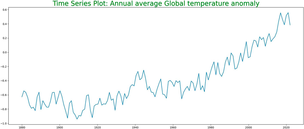
Figure 1 shows the time-series plot for the annual average global temperature anomaly. Since we are considering the annual average temperature anomalies, this graph does not have seasonality. Here, we can observe that earlier, the global temperature anomaly had a trend which was oscillating about some average value until 1960. However, since 1960, there has been a clear uptrend in the global temperature anomaly graph. It has increased in significant amounts, and thus, predicting future data for global temperature anomaly is very important.

FIGURE 1

FIGURE 1. Time series of global temperature anomaly data.

Figure 2A shows the autocorrelation function for the global temperature anomaly time series. The autocorrelation values for the first 20 lags can be seen. Here, the shaded region shows the threshold. In this graph, we can see that the autocorrelation declines slowly. Therefore, there is a possibility that the time series is not stationary, and the spikes of the ACF plot are over the threshold region.

FIGURE 2

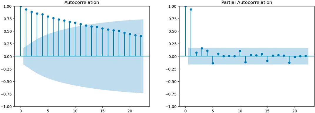
FIGURE 2. ACF and PACF for global temperature data. (A) Autocorrelation functions for global temperature data. (B) Partial autocorrelation function.

Figure 2B shows the PACF for the time series for the global temperature anomaly. Here, the first two lags are outside the threshold, and then the PACF shows a sudden drop such that all other lags have PACFs inside the threshold.

Using the ADF test (Mushtaq, 2011), we will check if the time series is stationary or not. For this, the Python package statsmodels.tsa.stattools was used. The result for the ADF test was generated as follows:

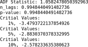
When we perform an ADF test on the data, the p-value obtained is greater than the significance level of 0.05, and the ADF statistic is higher than any of the critical values; that means there is no reason to reject the null hypothesis. Therefore, the time series is in fact non-stationary.

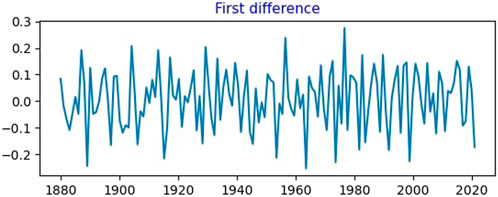
Thus, we attempt to find a stationary time series. For that, we take the first difference of the given data. Figure 3 shows the first difference of the given time series. It is certainly not up-trending. It shows the mean reversion behavior throughout the data.

FIGURE 3

FIGURE 3. First difference time series of global temperature anomaly data.

Additionally, we plot the autocorrelation for the first difference time series (Figure 4A). Here, after the first lag, we observed a sudden sharp decrease in the ACF, although there is very less difference between the second and the third lag. Almost all lags after that have ACFs within the threshold value. However, the second and third lags have values outside the threshold. Then, we plot the partial autocorrelation for the first difference time series (Figure 4B). We notice that after the first lag, the PACF shows a sudden decrease, but it decays slowly after that. The first four lags are outside the threshold. This shows that it is not a good model for the given time series.

FIGURE 4

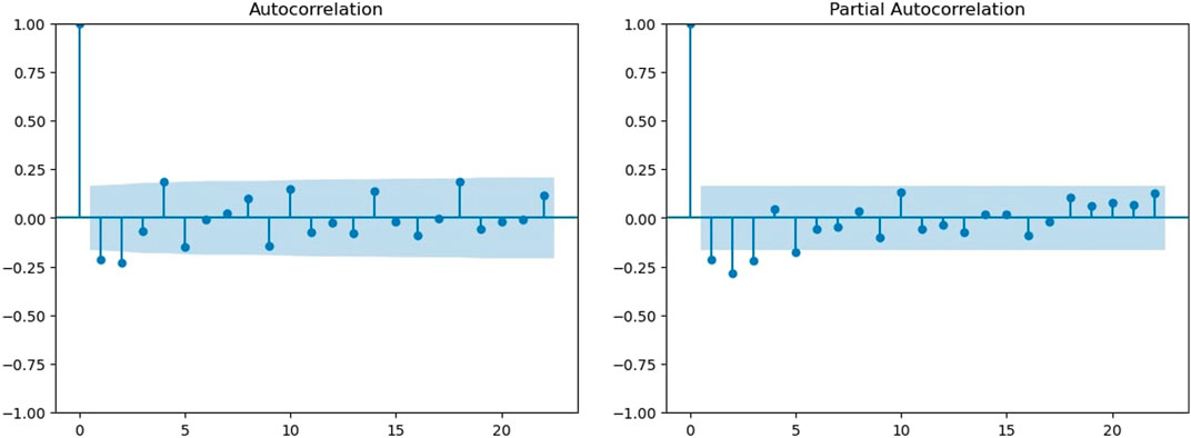
FIGURE 4. ACF and PACF of first differences. (A) ACF of the first difference. (B) PACF of the first difference.

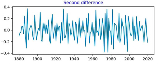
Figure 5 shows the second difference for global temperature data. This also shows the mean reversion. Furthermore, we plot the ACF and PACF for the second difference. Figure 6A shows the ACF for the second difference time series. Here, the first two lags are much outside the threshold by magnitudes. Lags after that are inside the threshold. From the behavior of the first two lags, we can say that there is a possibility that the time series is over-differenced. Figure 6B shows the PACF graph for the second difference time series. The first four lags here are outside the threshold, and they have very high magnitudes compared to the threshold. This confirms that the time series is overly differenced here, and thus, this is not the best fitted model for the given global data temperature.

FIGURE 5

FIGURE 5. Second difference time series of global temperature data.

FIGURE 6

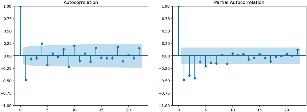
FIGURE 6. ACF and PACF of second differences. (A) ACF of the second difference. (B) PACF of the second difference.

4.1 Fitting an AR (1) model

We attempt to fit the AR (1) model in the given data using the auto_arima function in Python. The following is the summary of the results:

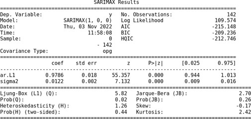
For the AR (1) model, we obtain the coefficients ϕ = 0.9786 and σ = 0.0122. This model fits with the skew −0.17 and kurtosis 2.42.

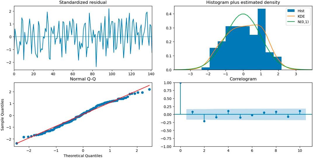
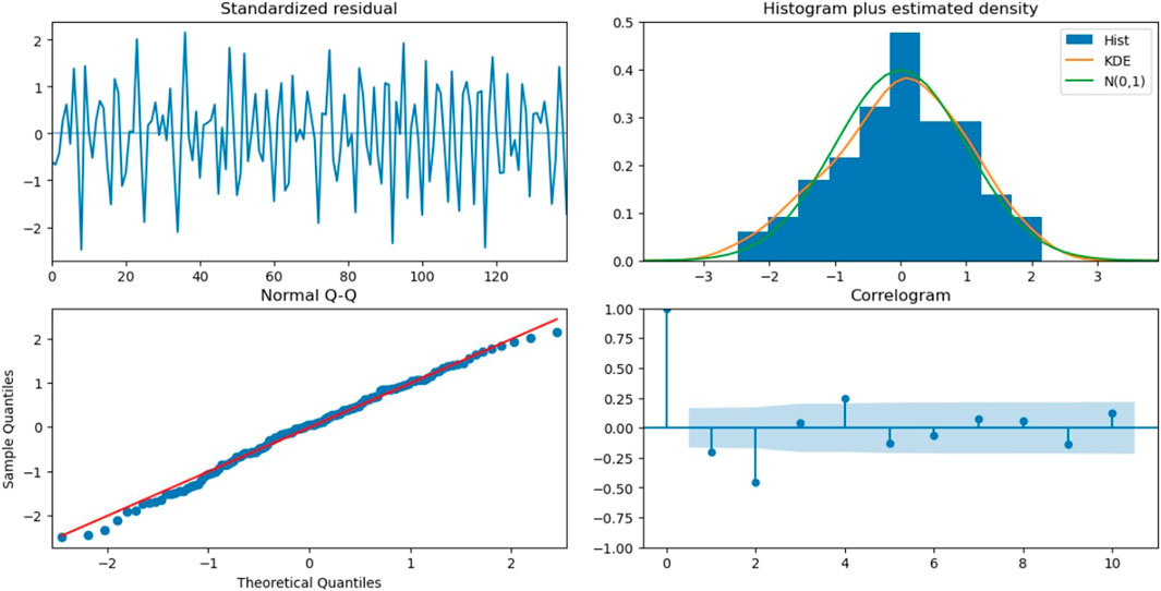
Figure 7 shows the diagnostics for the AR (1) model. The first figure shows us standardized residuals. The second figure shows the histogram for the data and standard normal (0,1) curve (in green) and the kernel density estimation (KDE) graph (in orange), which smooths the given data. Third is the normal Q-Q plot, where we can clearly observe that most of the sample quantiles and theoretical quantiles fit the normal distribution near the mean. However, outside the two standard deviations, it deviates from the reference line. Also, as we move away from the first to the second standard deviation, the data points start moving away from the reference line. Finally, we have a correlogram. Here, we can observe that this ACF graph is very similar to the ACF plot of the first difference of the original time series, so this is not the best fitting model, and we need to find a better model for these data.

FIGURE 7

FIGURE 7. Diagnostics for the AR (1) model.

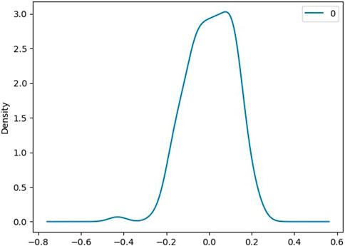
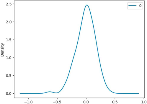
Figure 8 shows the density of residuals. Most of the residuals are near 0. Also, from the residual analysis, we can observe that the maximum value we have for residuals for the AR (1) model is 0.266279.

FIGURE 8

FIGURE 8. Density of residuals for AR (1).

4.2 Fitting ARMA (1,1) model

To obtain a better fit, we attempt to fit the ARMA (1,1) model in the given data using the auto_arima function in Python. The following is the summary of the results:

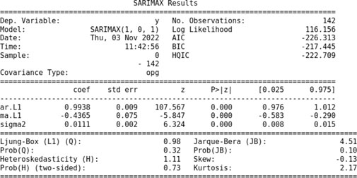
For the ARMA (1,1) model, we obtain the coefficients ϕ = 0.9938, θ = −0.4365, and σ = 0.0111. This model fits with the skew −0.13 and kurtosis 2.17.

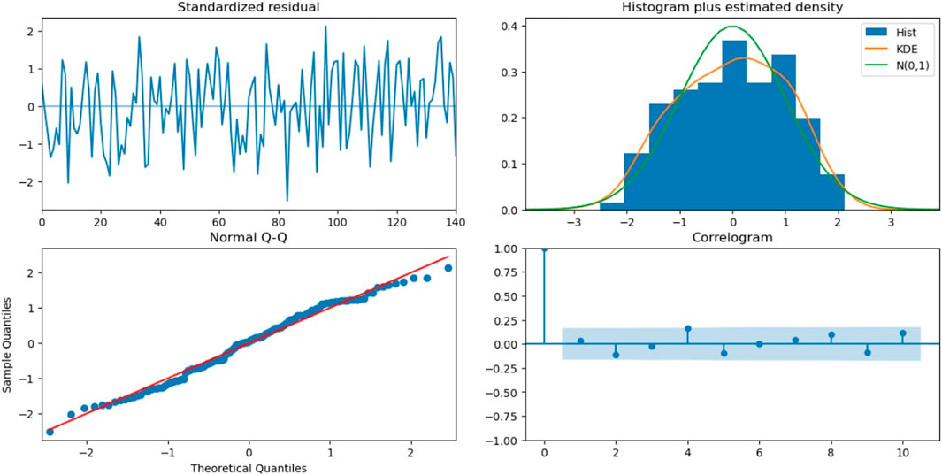
Figure 9 shows the diagnostics for the ARMA (1,1) model. The first figure shows the standardized residuals. Comparing the histogram of ARMA (1,1) to that of AR (1), we can see that the KDE graph fits better and is closer to the standard normal graph. In the third graph, we can see that most of the sample quantiles and theoretical quantiles fit the normal distribution near the mean. Here, between the first and second standard deviation, very few points are away from the reference line. This plot clearly shows that as compared to the AR (1) graph, ARMA (1,1) has a better fit to the given data. The correlogram here is different from the ACF plot of the original time series, and the second lag is inside the threshold.

FIGURE 9

FIGURE 9. Diagnostics for the ARMA (1,1) model.

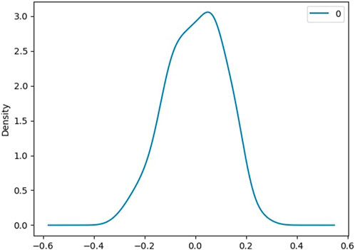
Figure 10 shows the density of residuals. Most of the residuals are near 0. From the analysis of residuals of ARMA (1,1), we can see that the maximum value we have for residuals is 0.232144, which is less than the maximum residual value for the AR (1) model. Thus, ARMA (1,1) is a much better model than AR (1).

FIGURE 10

FIGURE 10. Density of residuals for ARMA (1,1).

4.3 Fitting ARIMA (1,1,1) and ARIMA (1,2,0) models

In general situations, we are aware that ARIMA (p, d, and q) models fit better than ARMA models. So, we attempt to fit ARIMA models with the difference 1 and 2 in the GISTEMP data. For d = 1, a simulation shows that ARIMA (1,1,1) is the best model, and for d = 2, we find ARIMA (1,2,0) as the best fitting model.

Similar to previous fittings, we attempt to fit the ARIMA (1,1,1) model using the auto_arima function in Python. The following is the summary of the results:

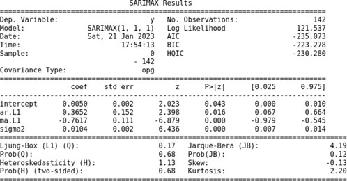
For the ARIMA (1,1,1) model, the coefficients are ϕ = 0.3652, θ = −0.7617, and σ = 0.0104. This model fits with the skew −0.13 and kurtosis 2.20.

Figure 11 shows the diagnostics for the ARIMA (1,1,1) model. The first figure shows the standardized residuals. Comparing the histogram of ARMA (1,1) to ARIMA (1,1,1), we can see that the KDE graph fits better in ARMA (1,1) and is closer to the standard normal graph. The normal Q-Q graph and the correlogram for ARIMA (1,1,1) do not look much different from that of ARMA (1,1).

FIGURE 11

FIGURE 11. Diagnostics for the ARMA (1,1,1) model.

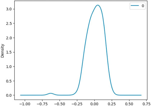
Figure 12 shows the density of residuals. Most of the residuals are near 0.1. From the analysis of residuals of ARIMA (1,1,1), we can see that the maximum value we have for residuals is 0.240199, which is higher than the maximum residual value for the ARMA (1,1) model. Thus, ARMA (1,1) is a better model than ARIMA (1,1,1).

FIGURE 12

FIGURE 12. Density of residuals for ARIMA (1,1,1).

Furthermore, we attempt to fit an ARIMA model with difference d = 2. The auto_arima function in Python shows that ARIMA (1,2,0) is the best fitting model for the given data, p ≤ 1 and q ≤ 1. When we fit ARIMA (1,2,0), we obtain the following results:

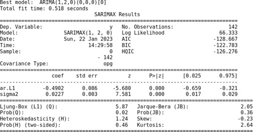
For the ARIMA (1,2,0) model, the coefficients are ϕ = −0.4902, θ = 0, and σ = 0.0227. This model fits with the skew −0.23 and kurtosis 2.64.

Figure 13 shows the diagnostics for the ARIMA (1,2,0) model. The first figure shows the standardized residuals. Comparing the histogram of ARMA (1,1) and ARIMA (1,2,0), we can see that the KDE graph here does not have a better fit. The normal Q-Q graph for ARIMA (1,2,0) does not look much different from that of ARMA (1,1). However, in a correlogram, we can see different behaviors of the ACF. Here, the ACF drops suddenly after the first lag, and the second and third lags are outside the threshold. After that, most of the lags are inside, but they are clearly not converging towards zero. This clearly shows that this model is not a good fit.

FIGURE 13

FIGURE 13. Diagnostics for the ARMA (1,2,0) model.

Furthermore, the density of residuals shown in Figure 14 confirms the result. Most of the residuals for ARIMA (1,2,0) are near 0. From the analysis of residuals, we can see that the maximum value we have for residuals is 0.398333, which is higher compared to the maximum residual value for the ARMA (1,1) model.

FIGURE 14

FIGURE 14. Density of residuals for ARIMA (1,2,0).

Hence, from the analysis of best fitting models for differences d = 1 and d = 2, i.e., ARIMA (1,1,1) and ARIMA (1,2,0) models, we can see that the ARMA (1,1) model is a better fit than those models.

5 Conclusion

Our new development of ARMA (1,1) based on uncertainty in the global mean anomaly due to uncertainties in the land and sea surface was analyzed and compared with AR (1), ARIMA (1,1,1), and ARIMA (1,2,0). In general theory, ARIMA (p, d, q) models are considered to have a better fit than that of ARMA (p, q) models. However, for the GISTEMP data from 1880 to the present, we found different results. Here, the ARMA (1,1) model is a better fitting model than the ARIMA (1,1,1) and ARIMA (1,2,0). Also, from simulations, it was evident that ARIMA (1,2,0) was a better fitting model than ARIMA (1,2,1), so it concludes the fact that ARMA (1,1) is a better model for the given data than ARIMA (1, d, 1) for d = 1 and d = 2.

The forecast for ARMA (1,1) is unbiased, and the forecast error variance increases without bounds as the lead time increases. For non-stationary series, when we forecast far into the future, we have a significant amount of uncertainty about the forecast. Moreover, from the normal Q-Q plot, correlograms, and KDE plot, we can say that the ARMA (1,1) model is a better fit. Furthermore, residual analysis confirms the result.

These results are true only for the GISTEMP data, and authors want to specify that the analysis in this article and results may or may not hold true for other data.

Data availability statement

The original contributions presented in the study are included in the article/Supplementary Material; further inquiries can be directed to the corresponding authors.

Author contributions

All authors listed have made a substantial, direct, and intellectual contribution to the work and approved it for publication.

Acknowledgments

The authors would like to thank Dr. Sang, Associate Prof., Department of Mathematics, the University of Mississippi for teaching the course on Time Series Analysis, where we learned and obtained the statistical idea about the time-series model.

Conflict of interest

The authors declare that the research was conducted in the absence of any commercial or financial relationships that could be construed as a potential conflict of interest.

Publisher’s note

All claims expressed in this article are solely those of the authors and do not necessarily represent those of their affiliated organizations, or those of the publisher, the editors, and the reviewers. Any product that may be evaluated in this article, or claim that may be made by its manufacturer, is not guaranteed or endorsed by the publisher.

Supplementary material

The Supplementary Material for this article can be found online at: https://www.frontiersin.org/articles/10.3389/fspas.2023.1098345/full#supplementary-material

References

Freeman, E., Woodruff, S. D., Worley, S. J., Lubker, S. J., Kent, E. C., Angel, W. E., et al. (2016). ICOADS release 3.0: A major update to the historical marine climate record. ICOADS release 3.0 A major update Hist. Mar. Clim. Rec. Int. J. Climatol. 37 (5), 2211–2232. doi:10.1002/joc.4775

CrossRef Full Text | Google Scholar

Hansen, J. E., and Lebedeff, S. (1987). Global trends of measured surface air temperature. J. Geophys. Res. 92, 13345–13372. doi:10.1029/JD092iD11p13345

CrossRef Full Text | Google Scholar

Hansen, J., Ruedy, R., Sato, M., and Lo, K. (2010). Global surface temperature change. Rev. Geophys. 48, RG4004. doi:10.1029/2010RG000345

CrossRef Full Text | Google Scholar

Hansen, J., Sato, M., Ruedy, R., Kharecha, P., Lacis, A., Miller, R., et al. (2007). Climate simulations for 1880–2003 with GISS modelE. Clim. Dyn. 29 (7-8), 661–696. doi:10.1007/s00382-007-0255-8

CrossRef Full Text | Google Scholar

Hasan, M., Khan, A. R., Ghosh, N., and Uddin -, M. (2015). On development of algorithm to design layout in facility layout planning problems. J. Phys. Sci. 20, 35–42.

Google Scholar

Hasan, Mahmud, Hossain, S., Ahamed, M. K., and Uddin, M. S. (2017). Sustainable way of choosing effective electronic devices using fuzzy TOPSIS method. Am. Acad. Sci. Res. J.35 (1), 342–351.

Google Scholar

Hawkins, E., Ortega, P., Suckling, E., Schurer, A., Hegerl, G., Jones, P., et al. (2017). Estimating changes in global temperature since the preindustrial period. Bull. Am. Meteorological Soc. 98 (9), 1841–1856. doi:10.1175/BAMS-D-16-0007.1

CrossRef Full Text | Google Scholar

Huang, B., Banzon, V. F., Freeman, E., Lawrimore, J., Liu, W., Peterson, T. C., et al. (2015). Extended reconstructed sea surface temperature version 4 (ERSSTv4). Part I: Upgrades and intercomparisons. J. Clim. 28 (3), 911–930. doi:10.1175/JCLI-D-14-00006.1

CrossRef Full Text | Google Scholar

Huang, B., Thorne, P. W., Smith, T. M., Liu, W., Lawrimore, J., Banzon, V. F., et al. (2016). Further exploring and quantifying uncertainties for extended reconstructed sea surface temperature (ERSST) version 4 (v4). J. Clim. 29 (9), 3119–3142. doi:10.1175/jcli-d-15-0430.1

CrossRef Full Text | Google Scholar

Lenssen, N., Schmidt, G., Hansen, J., Menne, M., Persin, A., Ruedy, R., et al. (2019). Improvements in the GISTEMP uncertainty model. J. Geophys. Res. Atmos. 124 (12), 6307–6326. doi:10.1029/2018JD029522

CrossRef Full Text | Google Scholar

Menne, M. J., Williams, C. N., Gleason, B. E., Rennie, J. J., and Lawrimore, J. H. (2018). The Global Historical Climatology Network monthly temperature dataset, version 4. J. Clim. 31, 9835–9854. doi:10.1175/jcli-d-18-0094.1

CrossRef Full Text | Google Scholar

Menne, M. J., Williams, C. N., Gleason, B. E., Rennie, J. J., and Lawrimore, J. H. (2018). The global historical climatology network monthlytemperature dataset, version 4. J. Clim. 31, 9835–9854. doi:10.1175/jcli-d-18-0094.1

CrossRef Full Text | Google Scholar

Menne, M. J., Williams, C. N., and Palecki, M. A. (2010). On the reliability of the U.S. surface temperature record. J. Geophys. Res. 115, D11108. doi:10.1029/2009jd013094

CrossRef Full Text | Google Scholar

Morice, C. P., Kennedy, J. J., Rayner, N. A., and Jones, P. D. (2012). Quantifying uncertainties in global and regional temperature change using an ensemble of observational estimates: The HadCRUT4 data set. J. Geophys. Res. 117, D08101. doi:10.1029/2011jd017187

CrossRef Full Text | Google Scholar

Mushtaq, R. (2011). Augmented Dickey fuller test. Available at SSRN: https://ssrn.com/abstract=1911068.

Google Scholar

Quattrochi, D. A., and Luvall, J. C. (2004). Thermal remote sensing in land surface processing. Boca Raton, FL, USA: CRC Press.

Google Scholar

Rayner, N. A., Parker, D. E., Horton, E. B., Folland, C. K., Alexander, L. V., Rowell, D. P., et al. (2003). Global analyses of sea surface temperature, sea ice, and night marine air temperature since the late nineteenth century. J. Geophys. Res. 108, 4407. doi:10.1029/2002JD002670

CrossRef Full Text | Google Scholar

Rohde1, R. A., Hausfather, Z., et al. (2021). The berkeley Earth land/Ocean temperature record.

Google Scholar

Shumway, R. H., and Stoffer, D. S. (2006). Time series analysis and its applications with R examples. 2nd Edition. Springer Texts in Statistics.

Google Scholar