A machine learning-based model for the next 3-day geomagnetic index (Kp) forecast

The 3-day Kp forecast product is important and necessary for space weather forecasts. There is some essential information that can be obtained from the 3-day Kp forecast product, such as the start time of the geomagnetic storm, the maximum storm level, and the storm duration. In this study, we aimed to predict the next 3-day Kp index based on the previous Kp time series and SDO/AIA 193 Å images. We prepared datasets from May 2010 to December 2019 for training and datasets from January 2020 to October 2022 for testing. The similarity parameters of the previous and current geomagnetic conditions between the samples are calculated and analyzed. We assumed that the paired samples with high-similarity parameters of the previous and current geomagnetic conditions would also have high-similarity parameters of the next 3-day geomagnetic conditions. Based on the assumption, we selected the three best similarity parameters through the feature selection process and adopted the scalable tree boosting system (XGBoost) to develop a prediction model. It took the similarity parameters of the previous and current geomagnetic conditions as input and provided the best match sample from the training subset as a forecast. For the next 3-day non-storm (maximum Kp $<$ 5) prediction period, our model reached an F1-score of 0.96. For the next 3-day storm (maximum Kp ≥ 5) prediction period, our model reached an F1-score of 0.82, a recall of 0.70, and a precision of 0.98.

1 Introduction

A geomagnetic storm is the consequence of solar wind disturbances originating from the Sun and impacting on geospace (Gonzalez et al., 1994; Perreault and Akasofu, 1978). The solar and interplanetary sources of the geomagnetic storms are related to coronal mass ejections [CMEs; (Gosling et al., 1991; Webb et al., 2000; Chen, 2011; Webb and Howard, 2012);] and the coronal hole high-speed stream (Tsurutani et al., 1995; Gonzalez et al., 1999; Tsurutani et al., 2006; Zhang et al., 2007). Geomagnetic storms can last from hours to days and sometimes lead to space weather effects, for example, the sudden enhancement of the electric currents in the magnetosphere and ionosphere, the severe changes of the relativistic electron fluxes in the Van Allen radiation belts, and the density enhancement in the upper atmosphere (Ritter et al., 2010; Mansilla, 2011; Xiong et al., 2015; Zhang et al., 2019).

Magnetic activity indices were designed to describe variations in the geomagnetic field, including the Kp index, ap index, and Ap index (Mayaud, 1980; Menvielle and Berthelier, 1991; Bartels, 2013a; Bartels, 2013b; Zhang et al., 2019). The planetary 3-hour-range Kp index ranging from 0 to 9 is calculated from 13 geomagnetic observatories between 44° and 60° northern or southern geomagnetic latitude. The 3-hour-range ap index is the equivalent range of the Kp index. The 1-day-range Ap index is calculated from an 8-point Ap index per day. Furthermore, Kp is a good representative for geomagnetic activity and is used to classify the geomagnetic conditions into categories (for example, minor storm, moderate, and major storm) in the Space Weather Prediction Center (SWPC) facilitated at the National Oceanic and Atmospheric Administration (NOAA) and the Space Environment Prediction Center (SEPC) facilitated at the National Space Science Center and the Chinese Academy of Sciences.

The Kp index and Ap index are also important inputs for physical-based geospace models, such as magnetosphere and plasmasphere models, and thermosphere and ionosphere models (Matzka et al., 2021). Compared with the 1-day-range Ap index, the 3-hour-range Kp index can provide more refined information on the geomagnetic activity, such as the start time of the geomagnetic storm, the maximum storm level, and the duration of the storm. Therefore, Kp index prediction is very important and necessary for space weather forecasts.

There are many models developed to predict geomagnetic activity on multiple time scales of hours to years based on statistical and machine learning methods (Feynman and Gu, 1986; Bala and Reiff, 2012; Wang et al., 2015; Luo et al., 2017; Tan et al., 2018; Shprits et al., 2019; Zhelavskaya et al., 2019; Chakraborty and Morley, 2020). However, only a few have been applied to the operational space weather forecast. At present, SWPC routinely provides products of a 45-day Ap index forecast¹, 27-day Ap index and the largest Kp index forecast², and 3-day Kp index forecast³. SEPC routinely provides products of a 27-day Ap index forecast⁴ and 3-h Kp index forecast in less than 3 h advance⁵. So far, there is no public algorithm designed for a 3-day Kp index forecast, and the conventional product of a 3-day Kp index forecast is only provided by SWPC.

The 3-day Kp index forecast is an essential and basic product in space weather forecasts. It contains 24 points in a 3-day period and describes the geomagnetic conditions with a 3-hour-range resolution. Considering the increasing demand for space weather forecasts, it is still important and necessary for the space weather community to develop prediction models that can provide the 3-day Kp index forecast product.

In this study, we aim to develop a model for the next 3-day Kp index time-series prediction. Here, we introduce the data preparation in Section 2, then develop a classification model based on machine-learning algorithms, and conduct prediction error analysis in Section 3. The conclusion and discussion are presented in Section 4.

2 Data and methodology

2.1 Data preparation

In this study, we used two kinds of data from May 2010 to October 2022, including the 3-hour Kp index from the National Oceanic and Atmospheric Administration (NOAA) and the 193Å wavelength images measured at the SDO/AIA (O’Dwyer et al., 2010; Lemen et al., 2012; Pesnell et al., 2012). They were divided into the training subset (including data from May 2010 to December 2019) and the testing subset (including data from January 2020 to October 2022). A prediction model was trained by the training subset and tested by the independent testing subset.

It should be mentioned that we only focus on the background solar wind (including the coronal hole high-speed streams and co-rotating interaction regions) in this study. Therefore, we removed the time periods when the geomagnetic conditions are affected by interplanetary coronal mass ejections (ICMEs), according to the near-Earth ICMEs list (Cane and Richardson, 2003; Richardson and Cane, 2010). For each day, we selected two samples according to the timepoints at 0:00 UTC and 12:00 UTC. Thus, we obtained 6,042 samples from the training subset and 1853 samples from the testing subset.

As shown in the flow chart in Figure 1, we prepared the 54-day Kp index time series before the current timepoint (T), and the AIA 193Å image was measured at T as inputs and we took the 3-day Kp index time series after T as outputs. Figure 2 shows how to divide the Kp time series into the previous 54-day Kp input and the next 3-day Kp output for the current T sample. Take the sample at 00:00 UTC on 22 Oct 2019 as an example, we took the Kp time series (432 points) from 00:00 UTC on August 29 to 00:00 UTC on October 22 as the input and the Kp time series (24 points) from 00:00 UTC on October 22 to 00:00 UTC on October 25 as the output. Figure 3 shows how to prepare the AIA 193Å image measured at T as input for the current T sample. Take the sample at 00:00 UTC on 22 Oct 2019 as an example, the observed image is shown in the top left panel. Then, a slice covering the [S40, N40] and [E40, W40] areas was cut from the observed image and shown in the top right panel. A median value was calculated based on the previous monthly slices. After all values above the median value in the slice at current T were replaced by 0, we obtained a slice as shown in the bottom left panel referring to the properties of coronal holes. The slice in the bottom left panel was then resized into a smaller size of 32 × 32 pixels and used as one of the inputs.

FIGURE 1

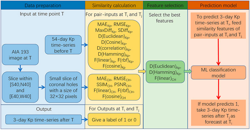
FIGURE 1. Flowchart of this study.

FIGURE 2

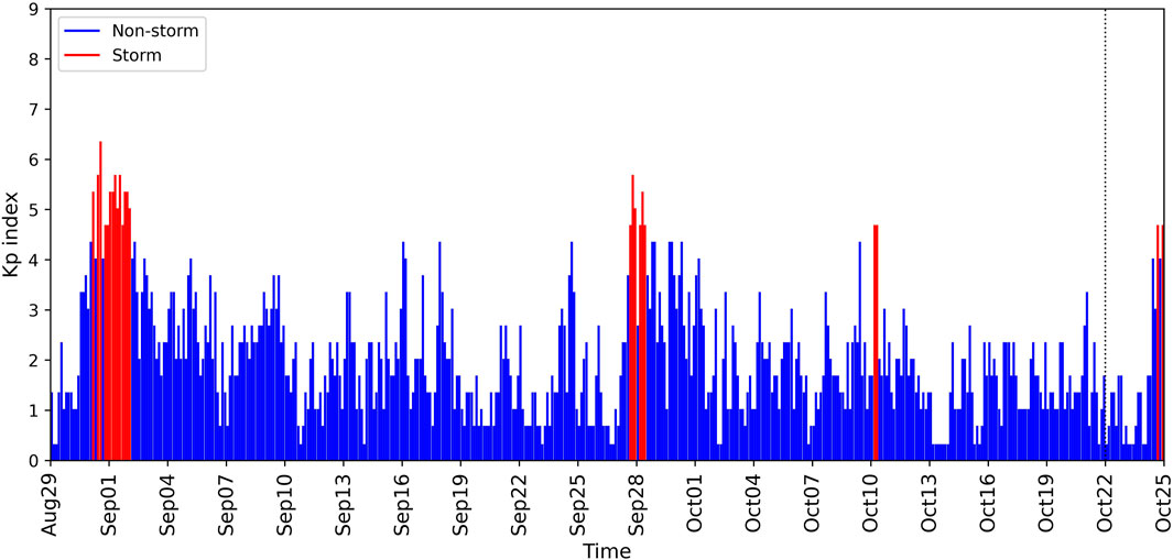
FIGURE 2. Illustration of preparing the 3-h Kp index time series for the current T at 00:00 UTC on 22 Oct 2019. The 3-h Kp index is represented by a blue (red) bar if it is related to the non-storm (geomagnetic storm) period. The black vertical line refers to the current time point T. The left side of the line refers to the previous 54-day Kp index time series (one of the model inputs). The right side of the line refers to the next 3-day Kp index time series (the model outputs).

FIGURE 3

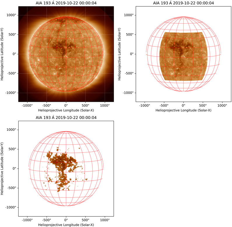
FIGURE 3. Illustration of preparing the AIA 193Å images. The upper left shows the 193Å images at 00:00:04 UTC on 22 Oct 2019 measured using SDO/AIA. The upper right shows the cut slice covering the [S40, N40] and [E40, W40] areas. After all values above the median in the slice are replaced by 0, the pre-processed slice referring to the coronal holes is shown in the bottom left.

To compare the difference between the training and testing subsets, we calculated the maximum value of the 3-day Kp output and took it as a representative for each sample. Then, we draw the sample distribution histogram in Figure 4. The blue and red bars represent the training and testing subsets, respectively. It was found that the maximum Kp of the samples in the two subsets had similar distribution properties. There were 1,614 (26.7%) and 390 (21.0%) storm samples (maximum Kp ≥ 5) in the training and testing subsets, respectively.

FIGURE 4

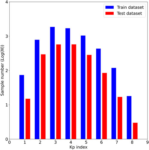
FIGURE 4. Sample distribution histogram at the training and testing subsets. The x-axis represents the maximum value of the 3-day Kp output for each sample. The y-axis represents the sample number.

2.2 Similarity calculation and labeling of sample pairs

Two samples at timepoints T_i and T_j from the training subset were called a pair (where the timepoint T_i was more than 3 days farther from T_j). For each sample at timepoint T_i, we picked up more than 5,000 other samples from the training subset to form sample pairs with it. All the samples that were within a 2-month interval of the current timepoint were excluded. As a result, we obtained more than 25 million sample pairs from the training subset.

We assume that if the inputs of two samples in a pair have high similarity (that is, their previous and current geomagnetic conditions are similar), their geomagnetic conditions in the next 3 days should be similar too. In this case, the two samples in the pair are similar to each other so that one sample can be a proper representative of the other one. In this study, the similarity parameters of the pair inputs were calculated and used to develop a model for the 3-day Kp forecast based on this assumption.

Figure 1 shows that based on the 54-day Kp time-series inputs, we derived 11 similarity parameters for each pair. The first two parameters were the mean absolute error (MAE_Kp) and the root mean square error (RMSE_Kp). They were calculated by the following formulas, where x and y represent the inputs of a pair at timepoints T_i and T_j, respectively:

$MAE\left(x,y\right)=\frac{1}{N}\sum _{i=1}^N\left|x_i-y_i\right|,(1)$

$RMSE\left(x,y\right)=\sqrt{\frac{1}{N}\sum _{i=1}^N{\left(x_i-y_i\right)}^2}.(2)$

The next two parameters were the maximum absolute error (MaxDiff_Kp) and the sum of the absolute error for the storm (Kp ≥ 5) period (SDiff_Kp). Also, four spatial distances were calculated, namely, the Euclidean distance (D (Euclidean)_Kp), cosine distance (D (Cosine)_Kp), correlation (D (Correlation)_Kp), and Hamming distance (D (Hamming)_Kp), by the following formulas and were taken as similarity parameters. The SciPy package⁶ was used to calculate these spatial distances.

$D\left(Euclidean\right)=\sqrt{\sum _{i=1}^N{\left(x_i-y_i\right)}^2}(3)$

$D\left(Cosine\right)=1-\frac{x\cdot y}{{‖x‖}_2{‖y‖}_2},(4)$

$D\left(Correlation\right)=1-\frac{\left(x-\bar{x}\right)\cdot \left(y-\bar{y}\right)}{{‖\left(x-\bar{x}\right)‖}_2{‖\left(y-\bar{y}\right)‖}_2}.(5)$

We also derived three features (Feature_KPCA(linear), Feature_KPCA(rbf), Feature_KPCA(cosine)) from each Kp time-series input using the kernel principle component analysis (KPCA) algorithm with the “linear,” “rbf,” and “cosine” kernel using the Scikit-learn package⁷. Through the KPCA algorithm, a Kp time-series input can be represented by a number (the feature). So, for each pair, we obtained two numbers (Feature_{x, KPCA(kernel)} and Feature_{y, KPCA(kernel)}) representing the Kp time-series pair inputs (x and y). Then, we calculated the absolute error of the two numbers and took it as the similarity parameter for the pair. In this way, we obtain three similarity parameters, namely, F (linear)_Kp, F (rbf)_Kp, and F (cosine)_Kp, by the following formula:

$\begin{array}{ll}\hfill F\left(kernel\right)& =Featur{e}_{x,KPCA\left(kernel\right)}\hfill \\ \hfill & -Featur{e}_{y,KPCA\left(kernel\right)},kernel\in \left\{linear,rgb,cosine\right\}.\hfill \end{array}(6)$

Figure 1 shows that based on the coronal holes image inputs, we derived another seven similarity parameters for each pair. The first two parameters were the mean absolute error (MAE_CH) and root mean square error (RMSE_CH), and were calculated by Formulas 1 and 2. The next two were the widely used image similarity parameters, such as structural index similarity (SSIM_CH) and peak signal-to-noise ratio (PSNR_CH), which were calculated using the Scikit-image package⁸. Then, in a similar way, we calculated the absolute error of the KPCA features derived by the image pair inputs using Formula 6 and took them as the similarity parameters, such as F (linear)_CH, F (rbf)_CH, and F (cosine)_CH.

Then, we obtained 18 similarity parameters from the pair inputs in the training subsets. Except for the correlation (D (Correlation)_Kp), structural index similarity (SSIM_CH), and peak signal-to-noise ratio (PSNR_CH), the larger the other 15 parameters, the higher similarity the pair inputs reach. Hence, it is the opposite for the correlation (D (Correlation)_Kp), structural index similarity (SSIM_CH), and peak signal-to-noise ratio (PSNR_CH). Then, we standardized the 18 similarity parameters independently by computing the relevant statistics on the pairs in the training subsets using the Scikit-learn package.

As we established the pair inputs and calculated the similarity parameters, the pair outputs (3-day Kp time series) should be analyzed and labeled as a number (1 or 0). Here, we adopted a batch labeling method according to the following principles:

1) For each sample at timepoint T_i, if the next 3-day geomagnetic conditions reached the storm level (maximum value of Kp ≥ 5), it is a storm sample. Otherwise, it is a non-storm sample.

2) For each sample at timepoint T_i, we picked up more than 5,000 other samples and formed pairs with them (denoted by T_i pairs). If a pair contains one storm sample and one non-storm sample, we considered the pair as a bad match and labeled the pair output as 0.

3) For each sample at timepoint T_i, we selected the top 100 pairs with the least mean absolute errors between their outputs (the next 3-day Kp time series) from the remaining T_i pairs. We considered those 100 pairs as good matches and labeled their pair outputs as 1. The remaining pairs were labeled as 0.

Finally, we prepared our dataset into a standard form consisting of inputs (18 similarity parameters) and output (binary labels) that is suitable for a binary classification task.

2.3 Feature selection of similarity parameters

Feature selection is a widely used approach in the machine learning community to select the best features from the dataset in which the model can perform better with less training time. In this study, we selected the best features by comparing the Pearson’s correlation of the 18 similarity parameters with the binary labels of the pairs using the SelectKBest from the Scikit-learn package. The correlations were standardized to scores ranging from 0 to 1, as shown in Figure 5.

FIGURE 5

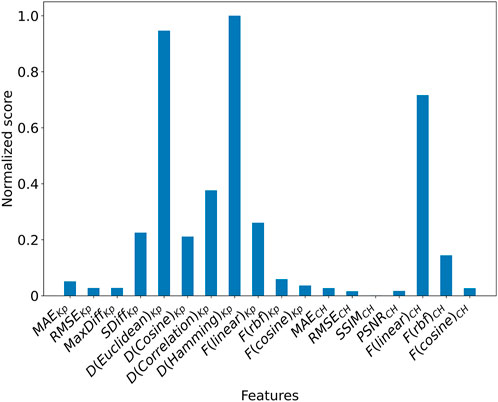
FIGURE 5. Scores of similarity of input pairs at the training dataset by feature selection.

It was found that there were three best features that had a significantly higher score than others. The top three best features were the Euclidean distance of the 54-day Kp time series (D (Euclidean)_Kp), the Hamming distance of the 54-day Kp time series (D (Hamming)_Kp), and the differences between the KPCA features of the current coronal hole images for each pair (F (linear)_CH). They were selected from the dataset and used for model development, as shown in the flowchart in Figure 1.

3 Model development and result analysis

3.1 Development of a classification model for sample pairs

After the three best features had been selected by feature selection, we determined to develop a classification model for pairs in the training subset to predict whether a pair of two samples is a good match or not. If the pair is a good match, their geomagnetic conditions are similar to each other so that one sample can be considered as a forecast of the other.

The scalable tree boosting system (XGBoost) is a widely used machine learning algorithm for binary classification tasks. It implements gradient boosting which performs additive optimization in functional space and incorporates a regularized model to prevent over-fitting (Chen and Guestrin, 2016).

We applied the XGBoost algorithm to develop a classification model using the Scikit-learn package⁹ to predict whether a pair of two samples is a good match or not. If the pair is a good match, their geomagnetic conditions are similar to each other so that one sample can be considered as a forecast of the other. Considering the “f1-weighted” (it is a balanced score of a standard binary classification task) as metrics, the best hyper-parameters of the XGBoost model are n_estimators = 0.01 and max _depth = 20.

As shown in Figure 1, to predict the 3-day Kp time series at T_i, we give a forecast of the 3-day Kp time series following the steps:

1) We pick up a sample at T_j to establish a pair and calculate the similarity parameters of the pair.

2) For the pair at T_i and T_j, the three similarity parameters are fed into the classification model. If the model predicts 1, the pair is a good match, whereas if the model predicts 0, it is not a good match.

3) If we find a good match, we take the 3-day Kp time series after T_j as forecast at T_i. Otherwise, we repeat the aforementioned steps.

We developed a prediction model using the training subset and applied the model on the testing subset from January 2020 to October 2022 and evaluated its performance. Both the geomagnetic storm prediction (maximum Kp ≥ 5) and non-storm (maximum Kp $<$ 5) prediction are important in space weather forecasts. Thus, we will evaluate the model for the geomagnetic storm prediction (maximum Kp ≥ 5) as well as the non-storm (maximum Kp $<$ 5) prediction tasks.

3.2 Evaluation metrics and model performance

For a binary classification task like the next 3-day geomagnetic storm (maximum Kp ≥ 5) prediction, the confusion matrix is shown in Table 1. The model is evaluated by its ability to predict the next 3-day geomagnetic storm, the first day (day 1) geomagnetic storm, the second day (day 2) geomagnetic storm, and the third day (day 3) geomagnetic storm. We also evaluate the model’s ability to predict the next 3-day non-storm conditions, the first day (day 1) of non-storm conditions, the second day (day 2) of non-storm conditions, and the third day (day 3) of non-storm conditions.

TABLE 1

TABLE 1. Confusion matrix for binary classification of the geomagnetic storm.

There are three metrics for binary classification used in the study, including precision, recall, and F1-score. They are calculated by the following formulas:

$recall=\frac{TP}{TP+FN},(7)$

$precision=\frac{TP}{TP+FP},(8)$

$F1=\frac{2\times precision\times recall}{precision+recall},(9)$

where the true positive (TP), false positive (FP), false negative (FN), and true negative (TN) are calculated following the confusion matrix, as shown in Table 1 for storm prediction and Table 2 for non-storm prediction. For example, for storm prediction, the higher the recall, the more storm samples have been correctly predicted. The higher the precision, the fewer false alarms have been made. An F1-score is a balance metric for recall and precision. A larger F1-score shows a better ability to classify a sample into the correct category.

TABLE 2

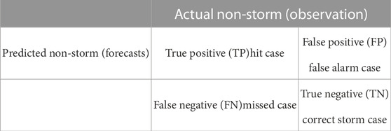
TABLE 2. Confusion matrix for the binary classification of non-storm.

The three metrics, recall, precision, and F1-score for the geomagnetic storm prediction task (considering the storm samples as positive samples) were listed as “For storm category (maximum Kp ≥ 5),” as shown in Table 3. The metrics for the non-storm prediction task (considering the non-storm samples as positive samples) were listed as “For non-storm category (maximum Kp $<$ 5),” as shown in Table 3. We found that

TABLE 3

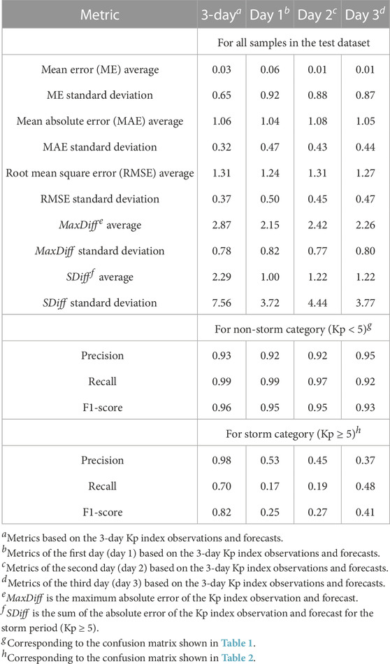
TABLE 3. Evaluation metrics for the best 3-day Kp index prediction model.

1) Our model reaches an F1-score of 0.96, a recall of 0.99, and a precision of 0.93 for the next 3-day period of non-storm category prediction and an F1-score of 0.82, a recall of 0.70, and a precision of 0.98 for the next 3-day period of storm category prediction.

2) However, both for the non-storm category and storm category, the three metrics (F1-score, recall, and precision) by our model are lower at the first day, second day, and third day period prediction than that in the next 3-day period prediction. It indicates that it is difficult to accurately predict the storm periods in a shorter time period (less than 3 days).

We also conducted an error analysis of the model forecasts with the observations in the testing dataset. For each sample (containing 24 points of the 3-hour Kp values) in the testing subset, we compared the forecasts with the observations by four statistics, including the mean absolute error (MAE), the root mean square error (RMSE), the maximum of the absolute error (MaxDiff), and the sum of the absolute error for the storm (Kp ≥ 5) period (SDiff). For 1853 samples in the testing subset, we calculated the average and standard deviation of the four statistics by the following formulas:

$Average\left(x\right)=\frac{1}{N}\sum _{i=1}^N{x}_i,(10)$

$StdDev\left(x\right)=\sqrt{\frac{1}{N-1}\sum _{i=1}^N\left(x_i-\bar{x}\right)}.(11)$

The eight statistics of the 3-day period, namely, day 1, day 2, and day 3 predictions, for all samples in the testing subset by our model are shown in Table 3. It was found that

1) The average and standard deviation of the mean error for the next 3-day Kp prediction is 0.03 and 0.65, respectively. The average and standard deviation of the mean absolute error for the next 3-day Kp prediction is 1.06 and 0.32, respectively.

2) The average and standard deviation of MaxDiff (the maximum absolute error of the 3-day Kp time-series) is 2.87 and 0.78, respectively.

Moreover, we compared our model results with the daily product of the 3-day Kp index forecasts provided by SWPC from 30 Nov 2020 to 27 Oct 2022. After we had removed the time-periods when the geomagnetic conditions are affected by interplanetary coronal mass ejections (ICMEs), there were 50 storm samples and 548 non-storm samples. Evaluation metrics for SWPC’s 3-day Kp index forecast products and results obtained by our model are shown in Table 4. It was found that

1) For the next 3-day prediction, our model provides a positive mean error average, while SWPC provides a negative mean error average. It indicates that statistically, our results are usually higher than the observations and SWPC’s products are usually lower than the observations.

2) For the next 3-day prediction, our model provides a mean error average of 1.13. It is slightly higher than the mean error average of 1.03 calculated from SWPC’s product.

3) Our model performs better than SWPC’s product for the three metrics (recall, precision, and F1-score) in the 3-day prediction. However, compared with SWPC’s results, our model had less recall and higher precision for the storm category in the first-day, second-day, and third-day predictions.

TABLE 4

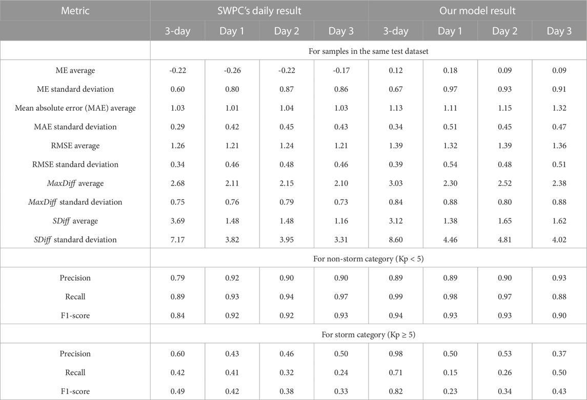
TABLE 4. Evaluation metrics for SWPC’s 3-day Kp index forecast products and our model.

4 Conclusion and discussion

In this study, we aimed to develop a model for the next 3-day Kp index time-series prediction based on the previous 54-day Kp time series and SDO/AIA 193 Å images. We prepared a dataset (6,042 samples) from May 2010 to December 2019 for training, and a dataset (1853 samples) from January 2020 to October 2022 for testing.

The similarity parameters of the previous and current geomagnetic conditions between the samples are calculated and analyzed, as well as the similarity parameters of the next 3-day geomagnetic conditions. We assumed that the paired samples with high similarity for the previous and current geomagnetic conditions would also have high similarity for the next 3-day geomagnetic conditions. Based on the assumption, we first selected the three best similarity parameters through the feature selection process and then adopted the XGBoost algorithm to develop a prediction model for the next 3-day Kp forecast. The model took the best three similarity parameters of the previous and current geomagnetic conditions as input and provided the best match sample from the training subset as a forecast for the next 3-day Kp time-series.

A prediction error analysis by our model was conducted. For the non-storm prediction, our model reached an F1-score of 0.96 for the next 3-day period and an F1-score over 0.92 for the first day, second day, and third day period. For the storm prediction, it reached an F1-score of 0.82, a recall of 0.70, and a precision of 0.98 for the next 3-day period.

We also compared our model results with the daily product of the 3-day Kp index forecasts provided by SWPC from 30 Nov 2020 to 27 Oct 2022. In statistics, our results were usually higher than the observations and SWPC’s products were usually lower than the observations. Compared with SWPC’s products for the next 3-day prediction, our model reached higher metrics (recall, precision, and F1-score). However, our model showed a higher mean error average in the next 3-day prediction, and less recall and higher precision for the storm category in the first-day, second-day, and third-day predictions.

This study established a prediction model that can be used to provide the 3-day Kp forecast product, which is important and necessary for space weather forecasts. There is some essential information that can be obtained from the 3-day Kp forecast product, such as the start time of the geomagnetic storm, the maximum storm level, and the duration of the storm. Therefore, it is a more refined product than the 3-day Ap forecast product. So far, the 3-day Kp forecast product is routinely provided by the Space Weather Prediction Center facilitated by the National Oceanic and Atmospheric Administration. Considering the increasing demand for space weather forecasts, more prediction models that can provide essential products should be developed.

However, the current model has limitations in accurately predicting the storm periods in a shorter time period (less than 3 days) which lead to lower evaluation metrics (recall, precision, and F1-score) in the first-day, second-day, and third-day predictions. In the future, we would like to improve the 3-day Kp forecast model by deriving more relevant similarity parameters of the geomagnetic conditions and adopting a complex machine learning algorithm such as a convolution neural network and long short-term memory.

Data availability statement

The original contributions presented in the study are included in the article/Supplementary Material; further inquiries can be directed to the corresponding author.

Author contributions

JW, BL, SL, and LS met the authorship criteria and agreed to be accountable for the content of the work.

Funding

JW was supported by the National Science Foundation of China (Grant No. 42074224), the youth innovation promotion association CAS, the Key Research Program of the Chinese Academy of Sciences (Grant No. ZDRE-KT-2021-3), and Pandeng Program of National Space Science Center of the Chinese Academy of Sciences.

Acknowledgments

The authors would like to thank the NOAA and the National Centers for Environmental Information that provided the geomagnetic indices. They authors thank the SDO/AIA team members that contributed to the SDO mission.

Conflict of interest

The authors declare that the research was conducted in the absence of any commercial or financial relationships that could be construed as a potential conflict of interest.

Publisher’s note

All claims expressed in this article are solely those of the authors and do not necessarily represent those of their affiliated organizations, or those of the publisher, the editors, and the reviewers. Any product that may be evaluated in this article, or claim that may be made by its manufacturer, is not guaranteed or endorsed by the publisher.

Footnotes

¹https://www.swpc.noaa.gov/products/usaf-45-day-ap-and-f107cm-flux-forecast

²https://www.swpc.noaa.gov/products/27-day-outlook-107-cm-radio-flux-and-geomagnetic-indices

³https://www.swpc.noaa.gov/products/3-day-geomagnetic-forecast

⁴http://www.sepc.ac.cn/eng/ApForecast.php

⁵http://www.sepc.ac.cn/eng/Kp3HPred.php

⁶https://docs.scipy.org/doc/scipy/index.html

⁷https://scikit-learn.org

⁸https://scikit-image.org/docs/stable/api/skimage.html

⁹https://scikit-learn.org

References

Bala, R., and Reiff, P. (2012). Improvements in short-term forecasting of geomagnetic activity. Space weather. 10, S06001. doi:10.1029/2012SW000779

CrossRef Full Text | Google Scholar

Bartels, J. (2013a). II – The technique of scaling indices k and q of geomagnetic activity. Geology 2013. doi:10.1016/B978-1-4832-1304-0.50006-3

CrossRef Full Text | Google Scholar

Bartels, J. (2013b). The geomagnetic measures for the time-variations of solar corpuscular radiation, described for use in correlation studies in other geophysical fields. Ann. Intern. Geophys. 4, 227. doi:10.1016/B978-1-4832-1304-0.50007-5

CrossRef Full Text | Google Scholar

Cane, H. V., and Richardson, I. G. (2003). Interplanetary coronal mass ejections in the near-Earth solar wind during 1996-2002. J. Geophys. Res. (Space Phys. 108, 1156. doi:10.1029/2002JA009817

CrossRef Full Text | Google Scholar

Chakraborty, S., and Morley, S. K. (2020). Probabilistic prediction of geomagnetic storms and the K_p index. J. Space Weather Space Clim. 10, 36. doi:10.1051/swsc/2020037

CrossRef Full Text | Google Scholar

Chen, P. F. (2011). Coronal mass ejections: Models and their observational basis. Living Rev. Sol. Phys. 8, 1. doi:10.12942/lrsp-2011-1

CrossRef Full Text | Google Scholar

Chen, T., and Guestrin, C. (2016). XGBoost: A scalable tree boosting System. arXiv e-prints , arXiv:1603.02754

Google Scholar

Feynman, J., and Gu, X. Y. (1986). Prediction of geomagnetic activity on time scales of one to ten years. Rev. Geophys. 24, 650–666. doi:10.1029/RG024i003p00650

CrossRef Full Text | Google Scholar

Gonzalez, W. D., Joselyn, J. A., Kamide, Y., Kroehl, H. W., Rostoker, G., Tsurutani, B. T., et al. (1994). What is a geomagnetic storm? J. Geophys. Res. 99, 5771–5792. doi:10.1029/93ja02867

CrossRef Full Text | Google Scholar

Gonzalez, W. D., Tsurutani, B. T., and Clúa de Gonzalez, A. L. (1999). Interplanetary origin of geomagnetic storms. Space Sci. Rev. 88, 529–562. doi:10.1023/a:1005160129098

CrossRef Full Text | Google Scholar

Gosling, J. T., McComas, D. J., Phillips, J. L., and Bame, S. J. (1991). Geomagnetic activity associated with Earth passage of interplanetary shock disturbances and coronal mass ejections. J. Geophys. Res. 96, 7831–7839. doi:10.1029/91ja00316

CrossRef Full Text | Google Scholar

Lemen, J. R., Title, A. M., Akin, D. J., Boerner, P. F., Chou, C., Drake, J. F., et al. (2012). The atmospheric imaging assembly (AIA) on the solar dynamics observatory (SDO). Sol. Phys. 275, 17–40. doi:10.1007/s11207-011-9776-8

CrossRef Full Text | Google Scholar

Luo, B., Liu, S., and Gong, J. (2017). Two empirical models for short-term forecast of Kp. Space weather. 15, 503–516. doi:10.1002/2016SW001585

CrossRef Full Text | Google Scholar

Mansilla, G. A. (2011). Some effects in the upper atmosphere during geomagnetic storms. Adv. Space Res. 47, 930–937. doi:10.1016/j.asr.2010.11.017

CrossRef Full Text | Google Scholar

Matzka, J., Stolle, C., Yamazaki, Y., Bronkalla, O., and Morschhauser, A. (2021). The geomagnetic kp index and derived indices of geomagnetic activity. Space weather. 19, e2020SW002641. doi:10.1029/2020SW002641

CrossRef Full Text | Google Scholar

Mayaud, P. N. (1980). Derivation, meaning, and use of geomagnetic indices. Wash. D.C. Am. Geophys. Union Geophys. Monogr. Ser. 22, 607. doi:10.1029/GM022.22.607M

CrossRef Full Text | Google Scholar

Menvielle, M., and Berthelier, A. (1991). The k-derived planetary indices: Description and availability. Rev. Geophys. 29, 415–432. doi:10.1029/91RG00994

CrossRef Full Text | Google Scholar

O’Dwyer, B., Del Zanna, G., Mason, H. E., Weber, M. A., and Tripathi, D. (2010). SDO/AIA response to coronal hole, quiet Sun, active region, and flare plasma. Astronomy Astrophysics 521, A21. doi:10.1051/0004-6361/201014872

CrossRef Full Text | Google Scholar

Perreault, P., and Akasofu, S. I. (1978). A study of geomagnetic storms. Geophys. J. 54, 547–573. doi:10.1111/j.1365-246x.1978.tb05494.x

CrossRef Full Text | Google Scholar

Pesnell, W. D., Thompson, B. J., and Chamberlin, P. C. (2012). The solar dynamics observatory (SDO). Sol. Phys. 275, 3–15. doi:10.1007/s11207-011-9841-3

CrossRef Full Text | Google Scholar

Richardson, I. G., and Cane, H. V. (2010). Near-Earth interplanetary coronal mass ejections during solar cycle 23 (1996 - 2009): Catalog and summary of properties. Sol. Phys. 264, 189–237. doi:10.1007/s11207-010-9568-6

CrossRef Full Text | Google Scholar

Ritter, P., Lühr, H., and Doornbos, E. (2010). Substorm-related thermospheric density and wind disturbances derived from CHAMP observations. Ann. Geophys. 28, 1207–1220. doi:10.5194/angeo-28-1207-2010

CrossRef Full Text | Google Scholar

Shprits, Y. Y., Vasile, R., and Zhelavskaya, I. S. (2019). Nowcasting and predicting the kp index using historical values and real-time observations. Space weather. 17, 1219–1229. doi:10.1029/2018SW002141

CrossRef Full Text | Google Scholar

Tan, Y., Hu, Q., Wang, Z., and Zhong, Q. (2018). Geomagnetic index kp forecasting with LSTM. Space weather. 16, 406–416. doi:10.1002/2017SW001764

CrossRef Full Text | Google Scholar

Tsurutani, B. T., Gonzalez, W. D., Gonzalez, A. L. C., Guarnieri, F. L., Gopalswamy, N., Grande, M., et al. (2006). Corotating solar wind streams and recurrent geomagnetic activity: A review. J. Geophys. Res. (Space Phys. 111, A07S01. doi:10.1029/2005JA011273

CrossRef Full Text | Google Scholar

Tsurutani, B. T., Gonzalez, W. D., Gonzalez, A. L. C., Tang, F., Arballo, J. K., and Okada, M. (1995). Interplanetary origin of geomagnetic activity in the declining phase of the solar cycle. J. Geophys. Res. 100, 21717–21733. doi:10.1029/95ja01476

CrossRef Full Text | Google Scholar

Wang, J., Zhong, Q., Liu, S., Miao, J., Liu, F., Li, Z., et al. (2015). Statistical analysis and verification of 3-hourly geomagnetic activity probability predictions. Space weather. 13, 831–852. doi:10.1002/2015SW001251

CrossRef Full Text | Google Scholar

Webb, D. F., Cliver, E. W., Crooker, N. U., Cry, O. C. S., and Thompson, B. J. (2000). Relationship of halo coronal mass ejections, magnetic clouds, and magnetic storms. J. Geophys. Res. 105, 7491–7508. doi:10.1029/1999ja000275

CrossRef Full Text | Google Scholar

Webb, D. F., and Howard, T. A. (2012). Coronal mass ejections: Observations. Living Rev. Sol. Phys. 9, 3. doi:10.1007/s41116-017-0009-6

CrossRef Full Text | Google Scholar

Xiong, C., Lühr, H., and Fejer, B. G. (2015). Global features of the disturbance winds during storm time deduced from CHAMP observations. J. Geophys. Res. (Space Phys. 120, 5137–5150. doi:10.1002/2015JA021302

CrossRef Full Text | Google Scholar

Zhang, J., Richardson, I. G., Webb, D. F., Gopalswamy, N., Huttunen, E., Kasper, J. C., et al. (2007). Solar and interplanetary sources of major geomagnetic storms (Dst <= -100 nT) during 1996-2005. J. Geophys. Res. (Space Phys. 112, A10102. doi:10.1029/2007JA012321

CrossRef Full Text | Google Scholar

Zhang, K., Li, X., Xiong, C., Meng, X., Li, X., Yuan, Y., et al. (2019). The influence of geomagnetic storm of 7-8 september 2017 on the swarm precise orbit determination. J. Geophys. Res. (Space Phys. 124, 6971–6984. doi:10.1029/2018JA026316

CrossRef Full Text | Google Scholar

Zhelavskaya, I. S., Vasile, R., Shprits, Y. Y., Stolle, C., and Matzka, J. (2019). Systematic analysis of machine learning and feature selection techniques for prediction of the kp index. Space weather. 17, 1461–1486. doi:10.1029/2019SW002271

CrossRef Full Text | Google Scholar