
94% of researchers rate our articles as excellent or good
Learn more about the work of our research integrity team to safeguard the quality of each article we publish.
Find out more
ORIGINAL RESEARCH article
Front. Astron. Space Sci. , 27 February 2023
Sec. Space Physics
Volume 10 - 2023 | https://doi.org/10.3389/fspas.2023.1062265
This article is part of the Research Topic Understanding the Causes of Asymmetries in Earth's Magnetosphere-Ionosphere System View all 11 articles
 Yu Hong1
 Yue Deng1*
 Qingyu Zhu2
 Astrid Maute2
 Marc R. Hairston3Colin Waters4
 Cheng Sheng1Daniel Welling1
 Ramon E. Lopez1
Inter-hemispheric asymmetry (IHA) in Earth’s ionosphere–thermosphere (IT) system can be associated with high-latitude forcing that intensifies during storm time, e.g., ion convection, auroral electron precipitation, and energy deposition, but a comprehensive understanding of the pathways that generate IHA in the IT is lacking. Numerical simulations can help address this issue, but accurate specification of high-latitude forcing is needed. In this study, we utilize the Active Magnetosphere and Planetary Electrodynamics Response Experiment-revised fieldaligned currents (FACs) to specify the high-latitude electric potential in the Global Ionosphere and Thermosphere Model (GITM) during the October 8–9, 2012, storm. Our result illustrates the advantages of the FAC-driven technique in capturing high-latitude ion drift, ion convection equatorial boundary, and the storm-time neutral density response observed by satellite. First, it is found that the cross-polar-cap potential, hemispheric power, and ion convection distribution can be highly asymmetric between two hemispheres with a clear By dependence in the convection equatorial boundary. Comparison with simulation based on mirror precipitation suggests that the convection distribution is more sensitive to FAC, while its intensity also depends on the ionospheric conductance-related precipitation. Second, the IHA in the neutral density response closely follows the IHA in the total Joule heating dissipation with a time delay. Stronger Joule heating deposited associated with greater high-latitude electric potential in the southern hemisphere during the focus period generates more neutral density as well, which provides some evidences that the high-latitude forcing could become the dominant factor to IHAs in the thermosphere when near the equinox. Our study improves the understanding of storm-time IHA in high-latitude forcing and the IT system.
Earth’s ionosphere–thermosphere (IT) system can be highly affected by high-latitude forcing, which plays a significant role in the energy and momentum transfer between solar wind and the magnetosphere–ionosphere (MI) system (Richmond, 2011). This forcing strongly intensifies during geomagnetic storms and is often characterized by large-scale anti-sunward convection flows and equatorward expansions of the auroral oval (Cowley and Lockwood, 1992; Fuller-Rowell et al., 1994). As a fundamental element in storm-time magnetospheric energy transport, the field-aligned currents (FACs) are associated with the ion convection patterns (Shi et al., 2020), along with an increase in Joule heating both locally and globally (Deng et al., 2018). As a global phenomenon, storm-time high-latitude forcing and its effects on the IT system can extend from the polar region to lower latitudes, with characteristic responses at different local times (LTs) and hemispheres (Pi et al., 1997; Jakowski et al., 2005; Basu et al., 2008; Astafyeva et al., 2014). One of the principal expansions is that when the interplanetary magnetic field (IMF) Bz suddenly turns negative, the enhanced magnetospheric convection cannot be fully shielded by the ring current in the magnetosphere and the region-2 FAC (Blanc et al., 1983; Goldstein et al., 2005). Different storm-related IT responses have been reported, such as electron density variations including polar patches and total electron content (TEC), traveling ionospheric disturbances (TIDs), and penetration electric fields (Tsurutani et al., 2008; Tulasi Ram et al., 2009; Jin and Xiong, 2020).
Due to Earth’s seasonal dipole tilt, the geomagnetic field configuration, and asymmetric high-latitude forcing (Hong et al., 2021), the storm-time IT responses can be significantly different between the Northern and Southern hemispheres, known as the IT system inter-hemispheric asymmetry (IHA). While all the causes are important, this study focuses on high-latitude forcing since the seasonal effect is considered to be reduced due to the data interval being near the equinox. It should be noted that the influence of the geomagnetic field is already included in high-latitude forcing since the forcing used in this study is the ultimate response of Earth’s upper atmosphere. We cannot separate the asymmetry of the original magnetosphere sources from the geomagnetic field effects regardless of which season it is (Förster and Cnossen, 2013). Previous studies have shown that high-latitude forcing strongly manifests asymmetries with complex temporal and spatial changes during geomagnetic storms (Burch et al., 1985; Reiff and Burch, 1985; Sandholt and Farrugia, 2007; Cousins and Shepherd, 2010), which could drastically affect the IT system in the two hemispheres. It has been emphasized by previous studies that the general FACs deduced from observations also exhibit hemispheric differences (Anderson et al., 2008; Green et al., 2009; Coxon et al., 2016; Workayehu et al., 2020). The IMF By component in the geocentric solar magnetospheric (GSM) coordinate system, i.e., dawn–dusk direction, is thought to be one main cause of a number of asymmetric features in the magnetosphere and IT system (Walsh et al., 2014). Studies also showed that IMF By causes obvious IHAs in auroral precipitation (Sandholt and Farrugia, 2007) and high-latitude Joule heating (McHarg et al., 2005). A full understanding of the IT system relies on knowledge of IHA. Despite these extensive studies, the global consequences and causes of the geomagnetic storm-related IHAs remain unknown.
General circulation models (GCMs) are widely used to study the IT system during geomagnetic storms. In order to specify the high-latitude forcing in GCMs, the most common approach is to utilize empirical models, e.g., using Weimer (2005) to specify convection patterns and using Fuller-Rowell and Evans (1987) or Newell et al. (2009) to specify auroral particle precipitation. However, since empirical models mainly describe the average conditions for a given state, they have issues in representing abrupt temporal changes or spatial distributions during a specific storm (Heelis and Maute, 2020). Typically, the two hemispheres are assumed to be mirror images considering a switch in IMF By and dipole tilt, and the data from the two hemispheres have been combined without considering differences in data coverage. Certainly, more realistic specifications of external forcing are required to accurately simulate the storm-time global IT responses. For example, magnetohydrodynamic (MHD) models can also be used to specify the high-latitude forcing of GCMs, such as the connection between the Lyon–Fedder–Mobarry (LFM) MHD model and the Thermosphere–Ionosphere-Electrodynamics General Circulation Model (TIEGCM), and the coupled magnetosphere–ionosphere–thermosphere (CMIT) model (Wang et al., 2004; Wiltberger et al., 2004). In addition, the Assimilative Mapping of Ionospheric Electrodynamics (AMIE) technique (Richmond and Kamide, 1988) can provide high-latitude electric potential and electron precipitation patterns used for driving GCMs (Lu et al., 2014; Lu et al., 2020). The Active Magnetosphere and Planetary Electrodynamics Response Experiment (AMPERE) gives another alternative way to calculate the high-latitude electric potential by using the derived FAC and pre-defined electron precipitation or ionospheric conductance patterns (Maute et al., 202l; Robinson et al., 2021; Zhu et al., 2022), which shows improved agreement between simulations and experimental data in driving GCMs for storms (Maute et al., 202l; Maute et al., 2022; Zhu et al., 2022b).
Motivated by the FAC-driven approach and AMIE electron precipitation patterns, the causes and consequences of IHAs of high-latitude forcing and IT responses during the October 8–9, 2012, storm have been investigated systematically with both data and models from over the high, middle, and low latitudes. The remaining part of this paper is organized as follows: Section 2 introduces the methodology of this study. Section 3 overviews the geophysical conditions for the October 8–9, 2012, geomagnetic storm in brief. Section 4 presents the main results of this study through comprehensive data–model and model–model comparisons. Section 5 summarizes the paper.
The present study utilizes integrated data from multi-instrument observations and models. The satellite observations are given in Section 2.1. Section 2.2 presents the GITM model. The newly developed FAC-driven procedure is given in Section 2.3. Section 2.4 illustrates how we determine the ion convection equatorial boundary according to DMSP observation.
Data from three Defense Meteorological Satellite Program (DMSP) satellites (i.e., F16, F17, and F18) are used in this study. They flew in sun-synchronous orbits at an altitude of ∼840 km with an inclination angle of ∼98.8° (Rich and Hairston, 1994) primarily in the dawn–dusk direction during the October 8–9, 2012, geomagnetic storm. The cross-track ion drift (Vy) is measured by using the onboard Special Sensor for Ions, Electrons, and Scintillation (SSIES), which has a temporal resolution of 1 s. In this study, the data with the quality flag of 1 (i.e., most reliable) are used. A linear baseline correction is applied to the original Vy data to remove some co-rotation effects and to ensure Vy is zero at 45° |magnetic latitude| (|MLAT|). Afterward, a 13-point sliding window is applied to the corrected data in order to reduce very-high-frequency fluctuations and extract the large-scale ion convection at high-latitude regions.
The Gravity Field and Steady-State Ocean Circulation Explorer (GOCE) satellite was launched on 17 March 2009. The satellite was a polar-orbiting satellite (inclination angle: 96.5°) and flew in a near-circular orbit with an altitude from 250 km to 280 km (Bruinsma et al., 2014). The solar local times (SLTs) of the ascending and descending nodes of the GOCE were about 19 and 07 h, respectively. The neutral mass density (hereafter, neutral density for simplicity) was measured by using an onboard accelerometer with a temporal resolution of 10 s (Doornbos et al., 2014). To reduce the variation caused by the satellite orbit altitude change, the neutral density data are normalized to a constant altitude of 270 km using the NRLMSIS 2.0 model (Emmert et al., 2021). More details of the density normalization technique can be found in Bruinsma et al. (2006).
The AMPERE high-latitude FAC densities are derived from the horizontal magnetic field perturbations measured by 66 Iridium satellites which are distributed along six longitudinally equally spaced orbital planes (Anderson et al., 2002). Each Iridium satellite flies in a near-polar orbit at an altitude of 780 km with an orbital period of 104 min. The radial current components are calculated by fitting the magnetic perturbations measured within a 10-min time window using spherical cap harmonic basis functions (Waters et al., 2001; Green et al., 2006; Waters et al., 2020). Specifically, the patterns are fitted with a longitude order of 5 and latitude order of 20 (i.e., 3°) between colatitude 0° and 60° in the Altitude-Adjusted Corrected Geomagnetic (AACGM) coordinates (Baker and Wing, 1989). The temporal resolution of the FAC data is up to 2 min, and the spatial resolution of the FAC data is 1° in MLAT and 1 h in the magnetic local time (MLT) (Anderson et al., 2014). In this study, AMPERE FAC densities with a magnitude below 0.2
The Global Ionosphere and Thermosphere Model (GITM) is a three-dimensional first-principle general circulation model for Earth’s thermosphere and ionosphere system (Ridley et al., 2006). The GITM solves continuity, momentum, and energy equations in a spherical coordinate framework to calculate the density, velocity, and temperature of neutrals, ions, and electrons. The GITM has a flexible grid size and can use a stretchable grid in latitude and altitude. Moreover, the GITM relaxes the hydrostatic assumption in the vertical direction, which allows for the evaluation of non-hydrostatic impacts on the IT system (Lin et al., 2017; Deng et al., 2021). The global ionospheric electrodynamic solver in the GITM is the NCAR-3D electrodynamic model (hereafter NCAR-3D, Maute and Richmond, 2017), which is coupled into the GITM by Zhu et al. (2019). More details about the GITM can be found in Ridley et al. (2006).
In this study, two main GITM simulations were run with different high-latitude electrodynamic forcing: driven by empirical models and by more realistic patterns. A summary of the high-latitude forcing settings of these runs is given in Table 1.
TABLE 1. Summary of simulations conducted in this study.
For run 1, the high-latitude electric potential is specified by the Weimer 2005 model (hereafter W05, Weimer, 2005), and electron precipitation is specified by the Auroral energy Spectrum and High-Latitude Electric field variabilitY (ASHLEY) model (Zhu et al., 2021). Both W05 and ASHLEY are driven by IMF and solar wind data. For run 2, the high-latitude electric potential is calculated using AMPERE FAC data and the electron precipitation is specified by the AMIE patterns. The data inputs to AMIE patterns for this storm event include the horizontal magnetic perturbations from 261 ground magnetometers (with 205 in the NH and 56 in the SH) and the electron precipitation measured by the Special Sensor of Ultraviolet Spectrographic Imager (SSUSI) onboard DMSP F16-18 satellites. Details about the AMIE can be found in Lu (2017). More realistic patterns which can resolve additional dynamic and spatial structures than the statistically averaged empirical models are used in run 2 as compared to run 1.
In each simulation, the GITM was run with a spatial resolution of 5° in geographic longitude, 2.5° in geographic latitude, and 1/3 scale height in altitude. The time step of both simulations is 2 s. Realistic IMF By and Bz, solar wind, and F10.7 data from the CDAWeb OMNI data product are used as model inputs. Specifically, in this study, the GITM simulations run 1 and run 2 are carried out with a 3-day pre-run (00UT (universal time) 10/01-00UT 10/03), a 5-day quiet time (00UT 10/03-00UT 10/08), and a 2-day event time (00UT 10/08 - 00UT 10/10) based on their corresponding high-latitude forcing. The purpose of a pre-run is to ramp up the model from an initial condition to a diurnally reproducible state during the time of interest (Deng and Ridley, 2006), and the outputs during that period typically are not used for scientific study.
This subsection gives a brief overview of the FAC-driven procedure used in this study, and details can be found in Maute et al. (2021) and Zhu et al. (2022). The first step is to calculate the high-latitude electric potential (
where
The superscripts N and S represent quantities in the Northern and Southern hemispheres, respectively. The specific definitions of the ionospheric conductivities
Once the high-latitude electric potential (
where
Here, the superscript T means the sum of quantities from both hemispheres.
In this study, the latitudinal expansion of the high-latitude ion convection to mid and low latitudes was investigated based on the cross-track ion drift Vy (nearly zonal direction below (|geographic latitude (GLAT)| = 70). The equatorial boundary is identified as the latitude at which the zonal ion drift suddenly gives a threshold. Heelis and Mohapatra (2009) suggested that the DMSP-observed zonal ion drift flow can be used to obtain the convection pattern equatorward expansion and contraction boundary, which is approximately consistent with the equatorward edge of the region-2 FAC. To quantitatively determine the equatorial boundary, a threshold of 15 m/s per degree in the latitudinal gradient of the zonal ion flow is adopted in this study (Heelis and Mohapatra, 2009). In addition, a criterion of 300 m/s greater than the quiet-time background flow is also applied in order to distinguish the enhancement from the quiet-time ion flow background (Hairston et al., 2016).
Figure 1 shows an example of the NH dusk-side ion convection equatorial boundary determined from the DMSP F16-measured zonal ion flow during the October 8, 2012, storm day. Specifically, the radius represents the GLAT, and the polar angle represents the geographic longitude (GLON) at the DMSP F16 fixed dusk-side LT, ∼18 SLT. The zonal ion flows were binned into 1° in GLAT between 10° and 80° GLAT and 2/3 h intervals (i.e., 10° in GLON). Figure 1A shows the quiet-time zonal ion flow background based on 7-day DMSP dusk-side measurements during October 1–7, 2012; Figure 1B shows the storm period zonal flow (around 14 trajectories per day) on October 8. Subtracting the zonal ion flow background 1A from the storm time 1B, the difference is shown in Figure 1C. By combining these two criteria described in the aforementioned paragraph, the ion convection boundary can be determined with black dots consistently for all longitudes, i.e., UT (UT = GLON/15–18 LT). Furthermore, we have also checked that using a larger or smaller threshold such as 400 m/s or 200 m/s only alters the boundary in the GLAT within 2° for this specific storm event.
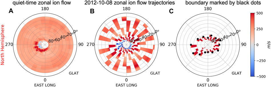
FIGURE 1. Example showing the identification of determining the ion convection equatorial boundaries in the Northern Hemispheric dusk side for DMSP F16. DMSP measured (A) quiet-time zonal ion flow background; (B) 2012–10–08 storm-time zonal ion flow trajectories; and (C) 2012–10–08 storm-time zonal ion flow after the identification. The positive and negative values represent the sunward and anti-sunward flows, respectively. The ion convection equatorial boundaries are marked by black dots in the third column (C). The radius represents the geographic latitude (GLAT), and the polar angle represents geographic longitude (GLON) at a fixed LT, ∼18 SLT, or universal time (UT = GLON/15.—18 LT).
Figure 2 shows the IMF components By and Bz, solar wind velocity Vx, interplanetary electric field (IEF, Ey = -Vx x Bz), SYM/H index, and auroral electrojet (AE) index for the moderate geomagnetic storm during October 8–9, 2012. As shown in Figure 2D, the storm sudden commencement (SSC) occurred at 05:16 UT on October 9 2012 and the SYM/H index reached ∼ −100 nT around 10:20 UT on October 8 during the first storm main phase (05:30 UT to 10:30 UT on October 8). The second main phase occurred between 18:00 UT on October 8 and 08:30 UT on October 9 during which the SYM/H index decreased to a minimum of ∼ −116 nT at 02:07 UT on October 9. During the second main phase, the IMF Bz component (Figure 2A) and IEF (Figure 2B) remained at around −15 nT and 5 mV/m, respectively. Meanwhile, the AE index showed rapid disturbances with basically above 600 nT and can reached up to 1400 nT (Figure 2C). The IMF By component stayed at around +8 nT before 01:20 UT and then quickly reversed to ∼ −8 nT. This study mainly focuses on the second main phase which offers us a great opportunity to examine the IMF By effects on the IHAs of high-latitude electrodynamic forcing and its impacts on the thermosphere.
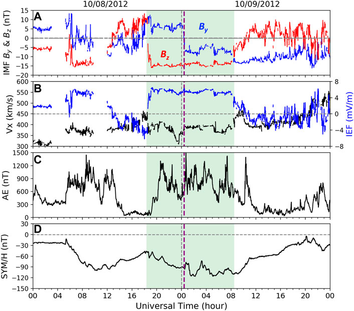
FIGURE 2. (A) Interplanetary magnetic field (IMF) By and Bz components, (B) solar wind velocity Vx and interplanetary electric field (IEF, E = −Vx x Bz), (C) auroral electrojet AE index, and (D) SYM/H index during October 8–9, 2012. The green shaded area highlights the period of interest in this study. The vertical purple dashed line marks the IMF By reversal time, which is around 00:20 UT on October 9 2012.
In Section 4.1, results from the empirical model-based run 1 (W05 and ASHLEY) and realistic pattern-driven run 2 (FAC-driven and AMIE electron precipitation) are compared with DMSP F16-18-observed cross-track ion drift Vy and the ion convection equatorial boundary. Section 4.2 illustrates the IHAs in high-latitude forcing, i.e., ion convection and auroral electron precipitation. The asymmetric storm phase response and By dependence of the ion convection equatorial boundary in both hemispheres are also investigated. The storm-time global evolutions of the thermospheric neutral density simulated by the GITM are compared with the GOCE satellite-measured result. The IHA and physical mechanism are examined in Section 4.3.
To determine how well the model output represents the ionospheric ion convection, a data–model comparison of the cross-track ion drift Vy has been conducted along DMSP trajectories during the focus period. As shown in Figure 3, six examples from DMSP F16-18 and the corresponding GITM runs are compared with the top and bottom panels representing the Northern and Southern hemispheres, respectively. For each plot, the black dots show the observed cross-track ion drift, and the blue and red curves represent the empirical model-based run 1 (W05) and realistic pattern-driven run 2 (FAC-driven and AMIE electron precipitation), respectively. In general, the cross-track Vy from both GITM runs is consistent with the DMSP results. When comparing the two sets of runs, the FAC-driven Vy from run 2 can better capture the realistic ion drifts in high latitudes than the W05-based results from run 1, especially inside the auroral zones.
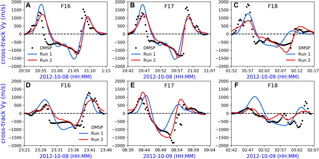
FIGURE 3. Comparison examples of the cross-track ion drift (Vy) along DMSP F16 (A,D), F17 (B,C), and F18 (C,F) trajectories. The black dots represent DMSP observations with a 13-point sliding window applied; blue and red lines represent GITM simulation run 1 and run 2, which are driven by empirical models and driven by data-based realistic patterns, respectively.
To investigate how GITM simulations capture the high-latitude ion drifts Vy from a statistical perspective, Figure 4 compares the simulated and measured cross-track ion drift at the region poleward of 45° |MLAT| from all DMSP trajectories during the focused period for runs 1 and 2. Linear fitting is performed on the data, and the slope (k) and y-intercept (b) are calculated. In addition, the Pearson correlation coefficient (r) and the root mean square error (RMSE) are also calculated. Basically, the cross-track ion drifts Vy from both GITM simulations have smaller magnitudes than the observed cross-track Vy since the slope of the best-fit line of the fitted line is much smaller than 1. This underestimation in the simulation results could be due to the underestimation of high-latitude forcing such as the FAC magnitude. This is a known property of AMPERE FAC data in the dusk-side R2 current. However, the slope of the best-fit line is slightly higher in run 2 than in run 1. Meanwhile, compared with run 1, run 2 shows a greater correlation (e.g., for DMSP F16 run 2 = 0.81 vs. run 1 = 0.68) and a smaller RMSE between the simulated and observed ion drifts (336.20 compared to 426.33) than run 1. Overall, Figure 4 indicates that the FAC-driven GITM simulation can better reproduce the high-latitude ion drift measured by DMSP satellites than the W05.
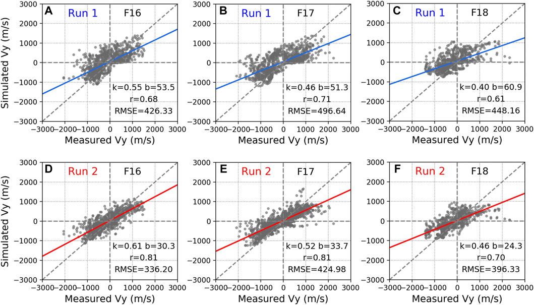
FIGURE 4. Scatter plots of DMSP-measured cross-track ion drift Vy versus corresponding GITM run 1 (top, driven by empirical models) and run 2 (bottom, driven by data-based patterns)- simulated Vy for all trajectories of F16 (A, D), F17 (B, E), and F18 (C, F) between 18 UT on October 8 and 09 UT on October 9. The straight lines represent the best-fit line. The slope (k), intercept (b), correlation efficient (r), and root mean square error (RMSE) are also shown in each plot.
The data–model comparisons of high-latitude ion convection given in Figure 3 and Figure 4 show a general consistency between the measured and simulated ion drift on the dawn and dusk sides, especially for run 2. Moreover, we would like to see how GITM simulations perform in response to the ion convection equatorial boundary. Figure 5 shows a scatterplot of the ion convection equatorial boundary in the GLAT for both hemispheres measured by DMSP F16 versus those from runs 1 and 2 during the focused storm period. In general, the simulations reproduce the DMSP-measured equatorward boundary latitudes well, with a better representation in run 2. Specifically, the correlation coefficients to DMSP F16 are 0.81 in the NH (Figure 5A) and 0.91 in the SH (Figure 5C) for run 1 and 0.92 in the NH (Figure 5B) and 0.95 in the SH (Figure 5D) for run 2. Moreover, as shown in Figures 5A, C, W05 has a clear underestimation of the convection expansion below 60° for the NH and at all the latitudes for the SH. This underestimation of the ion convection equatorial boundary may have some effects on other electrodynamical processes such as the ion-neutral interactions in that region. Overall, both runs show good agreement with the DMSP-observed convection equatorial boundary. The comparison between runs 1 and 2 is to give the community a rough idea about how well the FAC-driven technique could improve high-latitude electric field specification which is also a justification for using the FAC-driven technique in this study. For later scientific studies in Section 4.2 and Section 4.3, we would like to focus on the GITM run 2 since it has advantages over run 1 as discussed. A summary of the statistical parameters from the data–model comparisons of the two runs can be found in Table 2.
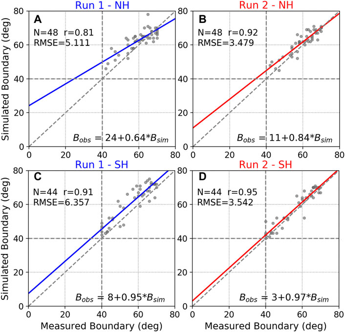
FIGURE 5. Scatter plots of the DMSP F16-measured ion convection equatorial boundary versus corresponding results from two GITM simulations run 1 (left, driven by empirical models) and run 2 (right, driven by data-based realistic patterns) during the October 8–9, 2012, geomagnetic storm for the northern (A, B) and southern (C, D) hemispheres. The straight lines represent the best-fit line. The number of dots (N), correlation coefficient (r), and root mean square errors (RMSE) are shown in the left-up corners, while the linear fitting equation is shown in the lower right corners.
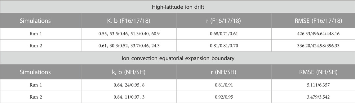
TABLE 2. Summary of data–model comparisons conducted in this paper.
Figure 6 shows the temporal variations of the cross-polar-cap potential (CPCP, top panel) and hemispheric power (HP, bottom panel) during October 8–9, 2012, from run 1 (left) and run 2 (right). The vertical dashed line marks the time when IMF By is reversed (00:20 UT on October 9) during the storm main phase we focused on in this study. All the red and blue lines correspond to the NH and SH, respectively. Following Hong et al. (2021), the asymmetry index (AI) is used to quantify the temporal changes of IHA for a given quantity:
where YNH and YSH stand for the quantity in the NH and SH, respectively.
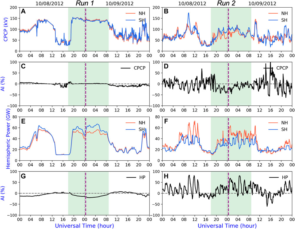
FIGURE 6. Inter-hemispheric comparisons of the (A, B) cross-polar-cap potential (CPCP) and (E, F) hemispheric power (HP) and their corresponding asymmetry index (AI) during the October 8–9, 2012, geomagnetic storm: (C, D) for CPCP and (G, H) for HP. The left column is for run 1 (driven by empirical models) and the right is for run 2 (driven by data-based realistic patterns). The vertical purple dashed line marks the IMF By reversal time during the storm main phase.
As shown in Figure 6A, CPCPs from run 1 are almost the same in the NH and SH during the focused period and the CPCP stays around 145 kV. As for run 2, significant asymmetries between the NH and SH can be seen in Figure 6B even for the recovery phase (e.g., after 12 UT on October 9). An evident asymmetry index (AI up to −50%, see Figures 6C, D) occurs in the CPCP during the focused period, especially before IMF By is reversed. In addition, the CPCP also exhibits more pronounced temporal variations than run 1. Similarly, as shown in the bottom two panels of Figures 6E, F, the hemispheric power in run 2 exhibits more dynamic variations and greater IHA than in run 1. The AIs can reach 75% and −22% in run 2 (Figure 6H) and run 1 (Figure 6G), respectively. Different from the CPCP, the HP tends to have greater AI in run 2 when the IMF By is negative (after 00:20 UT on October 9). Additionally, the HP in the NH is generally larger than that in the SH in run 2 while the opposite is true in run 1. This is probably due to the fact that the empirical model is mainly dependent on the given IMF, solar wind, and input seasonal conditions. Another reason is that, as described in Section 2.2, the AMIE patterns have better data coverage from the NH than that in the SH.
To our knowledge, the IHAs in high-latitude forcing could be due to the combined action of the season-related dipole tilt and the non-zero By component, which contribute to the asymmetric interaction in the dayside reconnection (Reistad et al., 2021). The well-known Dungey cycle suggests that the distribution of the open magnetic field flux in the two hemispheres should be the same. However, observations showed that the open magnetic flux in the polar cap is often distributed differently between the Northern and Southern hemispheres. Global auroral images from Polar and IMAGE satellites show different polar cap shapes, indicating hemispherically asymmetric distribution of open flux (Laundal and Østgaard, 2009). This is particularly true when there is an east–west component of the IMF (IMF By) (Tenfjord et al., 2015). The lobe reconnection due to IMF By causes the magnetic flux to build up asymmetrically (Lu et al., 1994). For example, the responding speed to the solar wind conditions in the two hemispheres can be different, which can result in different temporal variations of the magnetic flux between the two hemispheres (Milan et al., 2020). Therefore, this phase mismatch may result in some instantaneous asymmetry of the CPCP while it should be reduced significantly when the response in both hemispheres is fully developed. In addition to the reconnection for the IMF By, the field line potential drops across the hemispheres, and the asymmetries in the current systems produced by differing ionospheric conductivities and neutral dynamos in two polar regions contribute to the possible asymmetry in the CPCP as well. Data–model comparisons are still absolutely crucial to validate the simulation results. While the GITM simulations are able to capture the fundamental features of the ion drifts at high latitudes and the convection boundaries at mid-latitudes, the potential strong asymmetry of the CPCP presented in our simulation has yet to be corroborated with realistic observations. We will make careful comparisons with SuperDARN and other measurements in the follow-on study.
An enhanced geomagnetic storm can lead to large perturbations in the high-latitude ion convection and then extend to lower latitudes. From Section 4.1.2, we have demonstrated that the ion convection equatorial boundary from DMSP observations and GITM simulations shows a fairly good agreement on both the dawn and dusk sides. To have a detailed picture of the UT variations during this storm, Figures 7A, B directly show the temporal variations of DMSP F16-measured ion convection boundary in GLAT on dawn and dusk sides during the focused IMF By reversed period (18 UT on October 8–10 UT on October 9). Over this period, the NH dawn-side convection boundary (red dashed line) only undergoes a small variation (<5°) around 63° N GLAT, while the dusk-side convection boundary can expand to as far as 45° N (red solid line). As for the SH, both the dawn and dusk sides expand to lower GLATs during this interval of time, with the observed lowest boundary at 45° S and 40° S, respectively. One of the most interesting features is that these two sides reach their lowest |GLAT| under opposite IMF By conditions: the dawn side first expands under positive By and then contracts during negative By (blue dashed line), while the dusk side shows the opposite (blue solid line). This result could be explained by the anti-correlated responses between the dawn and dusk sides to By (e.g., Cowley, 1981; Reiff and Burch, 1985; Kabin et al., 2003; Tenfjord et al., 2015), the SH dawn-side convection cell is much stronger than the dusk-side cell under positive By, while the dusk side is more favorable under negative By in the SH.
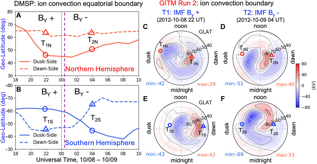
FIGURE 7. The left linear figure shows the temporal variations of the ion convection equatorial boundary along DMSP F16 ascending tracks, i.e., dusk side (solid lines) and descending tracks, i.e., dawn side (dashed lines) for both Northern [(A), red lines] and Southern [(B), blue lines] Hemispheres. The vertical purple dashed line marks the IMF By reversal time from positive to negative at around 00:20 UT 9 October 2012. Snapshots of the FAC-driven convection patterns in the Northern (top right) and Southern (bottom right) hemispheres under different IMF conditions: IMF By positive (C, E), 22 UT on October 8) and IMF By negative [(D, F), 04 UT on October 9]. The circle and triangle symbols refer to the dusk side and dawn side, respectively, under two different IMF By conditions.
In terms of the ion convection boundary comparisons between the two hemispheres, the temporal expansion in the NH dusk side (7A) follows a similar tendency to changes in the SH dawn side (7B), especially under positive IMF By. This could be the result of reversed By responses in the two hemispheres (Cousins and Shepherd, 2010), a stronger convection cell on average expands to lower latitudes. On the other hand, in contrast to the expansion in the SH dusk side (7b), the NH dawn-side convection expansion (7a) seems to be less important, implying a relatively stable convection cell on the dawn side. Moreover, this response is much stronger in the SH than in the NH, suggesting a stronger By dependence of the two cells in the SH (Burch et al., 1985). A possible explanation to the dawn–dusk asymmetry and IHA in the expansion is that the ion convection is subject to asymmetries in FACs and ionospheric conductivities. However, these line plots represent a limited view of ion convection pattern variation at two fixed LTs. The aforementioned hemispheric asymmetries between the NH and SH on both dusk and dawn sides will be further discussed in the following section.
To better understand the spatiotemporal variations of the ion convection patterns, Figures 7C–F present polar-view snapshots of the 2-D convection patterns from realistic pattern-driven GITM run 2 in both hemispheres under positive By at 22 UT October 8 (T1, left) and negative By at 04 UT October 9 (T2, right) from run 2. It can be seen in Figures 7E, F that the SH ion convection strengths and their expansions have obvious responses to IMF By. From T1 IMF By positive to T2 By negative, the dawn-side cell decreased from a maxima value of 42 kV (e) to 33 kV (f) associated with the dawn-side boundary contracted from ∼45oS (b and e, blue triangle) to 67oS (b and f, blue triangle). Similarly, for the dusk side, the cell with a minimum value −43 kV (e) with respect to −69 kV (f) leads to an expanded dusk-side boundary to much lower at ∼ 42oS (b and f, blue circle). However, as shown in Figures 7C, D, a stronger dusk-cell with minima value −51 kV (d) corresponds to a shrinking convection boundary (a and d, red circle). Furthermore, the dawn-cell increased from 29 kV (c) to 40 kV (d) with subtle changes in the boundary location. Again, the NH displays a clear stretch of the dawn-side cell in the noon–midnight direction instead of an equatorward expansion, which could explain the static phenomena along the DMSP F16 trajectory on the NH dawn side as shown in Figure 7A (red dashed line). This result suggests that it might be insufficient to determine the storm period ion convection expansion based on only the dawn and dusk LTs. Overall, the ion convection pattern simulated by the GITM for these two specific periods is in general agreement with the observed convection boundary expansions. Moreover, a stronger convection cell does not necessarily associate with a lower equatorial boundary.
In addition, we also conducted data–model comparisons of the equatorial boundary expansion at specific times. As shown in both the linear and polar plots, the red and blue triangles refer to the dawn side for the NH and SH, respectively. Similarly, the red and blue circles refer to the NH and SH but for the dusk side. The snapshot times T1 and T2 represent the corresponding positive By case at ∼ 22 UT on October 8 and negative By case ∼04 UT on October 9, respectively, which are marked in the left line plots. The subscripts N and S refer to the NH and SH, respectively. The boundary expansion features in the 2D contour from FAC-driven GITM run 2 are in a good agreement with the line plots from the DMSP F16 observations. For example, the blue triangle T2S (Figure 7B, dawn side) almost overlaps the expansion of the dawn-side potential cell (Figure 7F, blue color) at around 67oS GLAT.
To identify the possible mechanisms for the observed IHAs in the ion convection patterns, as well as their equatorial boundaries, a separation of the FAC and auroral electron precipitation (associated with the ionospheric conductance) is needed. In reality, the high-latitude FAC and auroral precipitation are connected and respond simultaneously to the changes in geophysical conditions, so it is impossible to completely separate the effects caused by these two variables. However, numerical simulations could help solve this issue by replacing the real forcing with symmetric patterns. We first examine the GITM run 2 (simulation setups in Table 1), which the high-latitude forcing is based on the FAC-driven potential and AMIE electron precipitation patterns. In GITM run 3, the AMIE electron precipitation patterns in the SH are replaced by the mirror precipitation patterns in the magnetic coordinate from the NH accordingly. Therefore, the differences in the SH between run 2 and run 3 illustrate the contributions from the auroral precipitation. Figure 8 shows the Southern hemispheric FAC-driven convection patterns and corresponding auroral energy flux from GITM run 2, run 3, and their differences at 04 UT on October 9 as an example. Specifically, due to the asymmetric electron precipitation, the auroral electron energy flux between the NH and SH is significantly different in both distributions and magnitudes: the SH has a continuous and complete aurora arc structure (Figure 8D) while the NH is more like a discrete aurora (Figure 8E). As shown in Figure 8F, the maxima difference in energy flux can vary from −45% to 55%. This result could be explained by the larger hemispheric power captured at that specific time (see Figure 6F); even the hemispheric power in the NH can be overwhelmingly superior to that in the SH during the focused period. However, the SH and NH electron energy flux-based ion convection (Figures 8A, B) illustrates quite similar distributions, as well as the maxima and minima values for the dawn (33 vs. 34 kV) and dusk (−69 vs. −67 kV) cells. Compared to Figure 8C, the differences caused by the asymmetric auroral precipitation can be ignored at this specific time. Moreover, by comparing the convection contour lines, one can find that the distributions, especially the equatorial boundaries of the convection, are more likely determined by the FAC patterns (R2 FAC edge) while its strength may also depend on the magnitude of the ionospheric conductance-associated precipitation. With this discussion, the effects from the FAC and auroral precipitation can be roughly isolated. It should be noted that this conclusion depends critically on the assumption of the FAC-driven procedure. Similar plots for all the UT times during the focus period indicate the same conclusion as the example time shown in Figure 8.
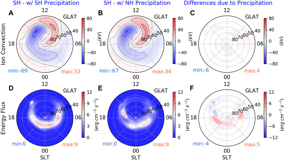
FIGURE 8. Snapshots of the FAC-driven convection patterns (top) for the Southern Hemisphere (SH) driven by different AMIE electron precipitation patterns at 04 UT on October 9 as an example: the SH precipitation itself (A), mirrored precipitation pattern in the geomagnetic field coordinate from the Northern hemisphere (NH, (B), and their difference (C). The corresponding energy flux of the precipitation patterns for the SH (D), NH (E), and their difference (F) are shown in the bottom.
To investigate the IHAs in the thermosphere during this storm, the neutral density observed by the GOCE satellite was first divided into ascending (dusk side) and descending (dawn side) trajectories. After that, the daily ascending trajectory data are binned into UT and GLAT grids with a bin size of 1 h and 1° in GLAT. We then applied a linear temporal interpolation in UT to project the data into uniformly distributed time series for both quiet-time background days and the storm-time days. Similarly, the approach is also used for GITM run 2-simulated neutral density extracted along the GOCE satellite trajectories for both quiet and storm days.
Figure 9A shows the observed neutral density response, dρ, on the dusk side as a function of UT and GLAT. The quiet-time neutral density background (given by the 2-day average of October 4 and 5) is subtracted from the storm-time observations. During the period of elevated geomagnetic activity, as indicated by the Ap and SYM/H indices shown in Figure 9D, it is clear that the observation generally shows density enhancements which last for several hours, and the neutral density increases after October 9. During the focus period (i.e., green shaded area), the NH shows dρ enhancements between 60o −80° N GLAT between 19:30 UT on October 8 and 00 UT on October 9 while the SH polar region represents stronger enhanced dρ at around 21:45 UT on October 8. The roughly 2-h difference in the responses between the NH and SH might be caused by asymmetric energy deposition such as the Joule heating in the two auroral regions. Another possibility is that the GOCE satellite trajectories are in different LTs in the NH and SH above 70° |GLAT|. Shortly after this period, both the neutral density in the NH and SH undergoes significant large-scale enhancements and the enhancements propagate equatorward and finally arrive at ∼30° S at 8 UT on October 9. Basically, the GOCE satellite-observed dusk-side dρ has some properties associated with IHA: the density-enhanced time, the density magnitudes, and the latitudinal propagation.
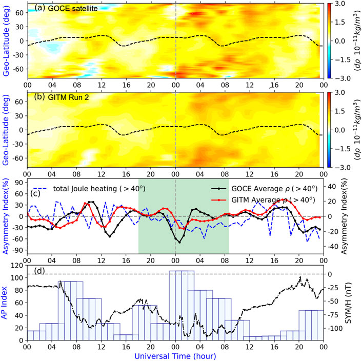
FIGURE 9. (A, B) Neutral density at the dusk side from the GOCE trajectory observation normalized at 270 km and GITM run 2 (driven by data-based realistic patterns)-simulated results sampled along the GOCE trajectory as functions of geographic latitude and universal times during the October 8–9, 2012, geomagnetic storm, respectively. The black dashed line refers to the dip equator. (C) Temporal changes of the asymmetry index for total Joule heating (hemispheric-integrated Joule heating, blue dashed line) from GITM run 2 (label on the left y-axis); the temporal changes of the asymmetry index for averaged density in the mid- and high-latitudes (>40° |GLAT|) based on the 2-D contour for GOCE (black dot line) and GITM run 2 (red dot line) with the label on the right y-axis. To have a general view of the storm-time response of the neutral density, (D) gives the geomagnetic activity information: the 3-hourly Ap index (blue) and SYM/H index (black).
Figure 9B is similar to Figure 9A but for the dρ from GITM run 2 (FAC-driven potential and AMIE electron precipitation). Specifically, the run 2-simulated neutral density over the same quite-time during October 4 and 5 is used as the quiet-time background subtracting for GITM as done for GOCE data. In general, the simulated dρ is consistent with the GOCE-measured results though some differences exist. For example, the much greater dρ on October 9 than on October 8 can be captured. In agreement with Figure 9A, Figure 9B shows an equatorward propagation of the neutral density enhancement. It is also worth noting that there are some differences in the data–model comparison: neutral density from GITM run 2 is smeared and has less mesoscale structures than those in the GOCE observations (Figure 9A), which may be due to three major reasons: 1) the latitudinal resolution in mid- and low latitudes of the observation (∼0.6 deg) is much higher than the simulation (2.5 deg); 2) the mesoscale forces may not be included in the simulations (Deng et al., 2019; Sheng et al., 2021); and 3) large-scale forcing is not perfect.
To quantify the asymmetric density features between the two hemispheres, Figure 9C shows the temporal changes of the AI for the averaged dρ at > 40° |GLAT| on the dusk side for both GOCE (black dot line) and GITM (red dot line). Apparent density asymmetries between the NH and SH can be identified, with the AI varying between −36% and 20% for the observations and between −18% and 20% for GITM results. As expected, the temporal changes of AI show some similarities and differences between GOCE and GITM results. Both the observational and simulation results show that the AI in dρ reaches its first maxima and minima at around 11 UT and 13 UT on October 8, respectively. During the storm period slightly after By is reversed, the asymmetry index reached its minimum value at ∼ -36% and −18% for the observational and simulation results, respectively. Moreover, a significant positive peak can be found during the recovery phase for both results but the magnitude in the GITM simulation seems to be much greater. As for the shaded focus period, the AI tends to be positive values (i.e., the NH has more density than the SH) under positive By rather than being significantly negative after By reversed into negative polarization, especially for the simulated results shown in the red line, implying that dρ might have some IMF By dependence associated with high-latitude forcing and energy dissipation.
To help understand the hemispheric difference in neutral density, the asymmetry index of the total (hemispheric-integrated) Joule heating >40° |GLAT| between the two hemispheres from GITM run 2 is also plotted in Figure 9C as a reference for the energy dissipation at high latitudes (blue dashed curves). The most remarkable feature is that negative AI (i.e., the SH has more total Joule heating than the NH) occurs shortly after the focus period and lasts almost to the end of the day, October 9, illustrating that the SH dusk side has more energy input during this period. Moreover, as shown in Figure 9C, between 12–20 UT on October 8, more Joule heating was deposited into the NH (positive AI), resulting in increased density in the NH in density dρ during 16–22 UT on October 8. Immediately after this, greater Joule heating was dissipated into the SH with the minima of AI (∼-60%) near 05 UT on October 9 in Joule heating. In general, the total Joule heating can lead to changes in neutral density enhancement, with 2–3 h of delay for the thermosphere to respond to the energy input change during storm times (Wang et al., 2020). On the basis of the aforementioned features, it can be summarized that the variations and IHA in the dρ could be significantly due to the contributions from the Joule heating dissipations.
The storm-time IT system responses are largely controlled by two factors: external high-latitude forcing from the solar wind–magnetosphere–ionosphere interaction and the local conditions in the thermosphere and its embedded ionosphere. Therefore, the IHAs in the thermosphere could also come from several other mechanisms as discussed in the introduction. As described by several previous papers (Laundal and Østgarrd, 2009; Ohtani et al., 2009; Reistad et al., 2015; Laundal et al., 2017), the intrinsic North–South differences in the geomagnetic field could introduce asymmetric interaction of MI coupling in the two hemispheres. It should be pointed out that the IHA due to asymmetric tilt angles and displacements between the two hemispheres is daily UT differences. For example, at any given UT, the two hemispheric auroral zones will be one near nighttime and the other located in the dayside, which implies different solar fluxes would also be concerned during this period. Certainly, the absolute neutral density variation is also subject to the background thermospheric density before the storm, which provides important preconditions (McGranaghan et al., 2014). Previous studies have shown that both the season and geomagnetic field can contribute to the IHAs in the thermospheric neutral density (Emmert, 2015). Further examination shows that no obvious IHAs or enhancements could be found in the neutral density and Joule heating during the quiet-time background, i.e., October 4 and 5 from both GOCE and GITM results; given its proximity to the equinox, the result reveals that the storm-time intensified high-latitude forcing and associated Joule heating could be the dominant factor causing the IHAs to the neutral density dρ in the thermosphere.
So far, we have discussed the storm-time responses in high-latitude forcing, Joule heating dissipation, and the thermosphere, all of which have significant IHAs as illustrated by measured and simulated results. To complete the pathways of IHAs from high-latitude forcing to Joule heating, similar to the inter-hemispheric comparisons in Figure 6, we conducted the same examination for the total FAC and total Joule heating (from run 2). As shown in the left part of Figures 10A, C, the total FAC indicates small positive asymmetry during the focused shaded period between the two hemispheres as expected for the equinox condition, with AI no more than 25%. In terms of the total Joule heating shown on the right, an overall negative AI (up to −75%, Figure 10D) can be found during the same period, indicating that more heating is dissipated into the SH. As a conversion between the electromagnetic energy and mechanical form, Joule heating is conventionally taken in the form
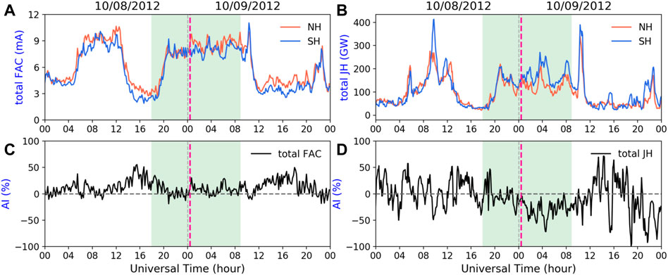
FIGURE 10. Inter-hemispheric comparisons of the total field-aligned current (FAC, (A), total Joule heating (B), and their corresponding asymmetry index (AI, (C, D) during the October 8–9, 2012, geomagnetic storm. All the results are from run 2 (driven by data-based realistic patterns) since run 2 has obvious advantages in reproducing the high-latitude forcing. The vertical purple dashed line marks the IMF By reversal time during the storm main phase.
The inter-hemispheric asymmetries in the global IT system have been investigated during the October 8–9, 2012, geomagnetic storm for a focused IMF By reversal period. The IHA in the high-latitude convection and auroral precipitation, the convection equatorial boundary, and the thermospheric neutral density have been investigated by combining data analysis and GITM simulations. The major conclusions are summarized as follows:
1) This study demonstrates the advantage of the FAC-driven technique in the global IT system study. Simulations based on realistic, spatial FAC patterns can better capture the high-latitude ion drift and the convection equatorial boundary than the empirical model-driven results. A summary of statistical parameters for the data–model comparisons of the two simulations is given in Table 2.
2) Significant IHAs have been identified in the FAC-driven simulation in both the high-latitude forcing and the IT system, with AI up to −50% in CPCP, 75% in hemispheric power, and −36% in neutral density. The IHAs show a By dependence, especially for the convection boundary.
3) By comparing FAC-driven convection patterns based on precipitation from the SH itself or the mirror pattern from the NH, our results suggest that the distribution of the ion convection, especially the equatorial boundary, is more likely to be determined by the R2 FAC edge while its intensity may also depend on the ionospheric conductance associated with aurora precipitation energy flux.
4) The FAC-driven case well-captures the storm-time thermospheric neutral density response and its IHA on the dusk side. Basically, the density response has some properties associated with IHA: the start time of the enhancement, the relative magnitudes, and the latitudinal propagations between the NH and SH. It is found that the IHA in the neutral density response follows the variations in total Joule heating and has a time delay of ∼3 h.
5) Previous studies have shown that both the season and geomagnetic field can determine IHAs in the thermosphere. Our study suggests that Joule heating associated with high-latitude forcing can become the dominant factor even during a moderate storm period when near the equinox.
We acknowledge the use of NASA/GSFC’s Space Physics Data Facility’s OMNIWeb (or CDAWeb or ftp) service, and OMNI data. The IMF and solar wind data can be found at (https://omniweb.gsfc.nasa.gov/). The AMPERE FAC data can be found at (https://ampere.jhuapl.edu/). The GOCE neutral density data can be found at (https://earth.esa.int/eogateway/missions/goce/data). The DMSP SSIES ion drift data are available at http://cedar.openmadrigal.org/. The data used in this study along with AMIE outputs and GITM simulation outputs can be found at https://zenodo.org/record/7475704#.Y6UlZhNKhR4.
YH conducted the data analysis and modeling studies. YD guided each step of this work and contributed to individual discussions of results. QZ coupled the NCAR-3D model into the GITM, added the FAC-driven capability to the NCAR-3Dynamo model, and created the AMIE electron precipitation pattern. AM developed the NCAR-3Dynamo module and the FAC-driven procedure. MH developed the identification of determining the equatorial boundary of ion convection. CW processed the Iridium satellite data and provided advice on differences between the hemisphere data fits. CS provided interpretation for the thermospheric neutral density performances. DW and RL assisted in the analysis of the storm event as experts in the research field of IHA and magnetosphere physics. All the co-authors contributed to the discussions, comments, and improvements to the manuscript.
This research conducted at the University of Texas at Arlington was supported by AFOSR through award FA9559-16-1-0364 and NASA through awards 80NSSC20K0195, 80NSSC20K1786, 80NSSC20K0606, 80GSFC22CA011, and 80NSSC22K0061. YH was also supported by the National Center for Atmospheric Research (NCAR) Advanced Study Program (ASP) Graduate Visitor Program Fellowship. QZ was supported by the NCAR ASP Postdoctoral Fellowship and NASA GOLD ICON Guest Investigators Program under grant 80NSSC22K0061 through the subaward 2021GC1619. YH and QZ were also supported by the NCAR Early Career Scientist Assembly Visitor Fund. AM was supported through AFOSR award FA9559-17-1-0248 and NASA award 80NSSC20K1784. This material is based on the work supported by the National Center for Atmospheric Research, which is a major facility sponsored by the National Science Foundation under Cooperative Agreement No. 1852977.
The authors appreciate the two reviewers for their valuable contributions in reviewing and improving this manuscript. They also thank Brian J. Anderson for valuable discussion on AMPERE FAC data. They would like to acknowledge high-performance computing support from Cheyenne (https://doi.org/10.5065/D6RX99HX) provided by the National Center for Atmospheric Research’s Computational and Information Systems Laboratory, sponsored by the National Science Foundation. They acknowledge support from the ISSI for the international team on “Multi-Scale Magnetosphere–Ionosphere–Thermosphere Interaction.”
The authors declare that the research was conducted in the absence of any commercial or financial relationships that could be construed as a potential conflict of interest.
All claims expressed in this article are solely those of the authors and do not necessarily represent those of their affiliated organizations, or those of the publisher, the editors, and the reviewers. Any product that may be evaluated in this article, or claim that may be made by its manufacturer, is not guaranteed or endorsed by the publisher.
Anderson, B. J., Takahashi, K., Kamei, T., Waters, C. L., and Toth, B. A. (2002). Birkeland current system key parameters derived from Iridium observations: Method and initial validation results. J. Geophys. Res. 107 (A6), 1079. doi:10.1029/2001JA000080
Anderson, B. J., Korth, H., Waters, C. L., Green, D. L., and Stauning, P. (2008). Statistical Birkeland current distributions from magnetic field observations by the Iridium constellation. Ann. Geophys. 26, 671–687. doi:10.5194/angeo-26-671-2008
Anderson, B. J., Korth, H., Waters, C. L., Green, D. L., Merkin, V. G., Barnes, R. J., et al. (2014). Development of large-scale birkeland currents determined from the active magnetosphere and planetary electrodynamics response experiment. Geophys. Res. Lett. 41, 3017–3025. doi:10.1002/2014GL059941
Astafyeva, E., Yasyukevich, Y., Maksikov, A., and Zhivetiev, I. (2014). Geomagnetic storms, super-storms, and their impacts on GPS-based navigation systems. Space Weather 12, 508–525. doi:10.1002/2014SW001072
Baker, K. B., and Wing, S. (1989). A new magnetic coordinate system for conjugate studies at high latitudes. J. Geophys. Res. 94 (A7), 9139–9143. doi:10.1029/JA094iA07p09139
Basu, Su., Basu, S., Makela, J. J., MacKenzie, E., Doherty, P., Wright, J. W., et al. (2008). Large magnetic storm-induced nighttime ionospheric flows at midlatitudes and their impacts on GPS-based navigation systems. J. Geophys. Res. 113, A00A06. doi:10.1029/2008JA013076
Blanc, M., Alcaydé, D., and Kelly, J. D. (1983). Magnetospheric convection effects at mid-latitudes: 2. A coordinated chatanika/saint-santin study of the april 10–14, 1978, magnetic storm. J. Geophys. Res. 88 (A1), 224–234. doi:10.1029/JA088iA01p00224
Bruinsma, S., Forbes, J. M., Nerem, R. S., and Zhang, X. (2006). Thermosphere density response to the 20–21 November 2003 solar and geomagnetic storm from CHAMP and GRACE accelerometer data. J. Geophys. Res. 111, A06303. doi:10.1029/2005JA011284
Bruinsma, S. L., Doornbos, E., and Bowman, B. R. (2014). Validation of GOCE densities and evaluation of thermosphere models. Adv. Space Res. 54, 576–585. doi:10.1016/j.asr.2014.04.008
Burch, J. L., Reiff, P. H., Menietti, J. D., Heelis, R. A., Hanson, W. B., Shawhan, S. D., et al. (1985). IMFBy-dependent plasma flow and birkeland currents in the dayside magnetosphere: 1. Dynamics explorer observations. J. Geophys. Res. 90 (A2), 1577–1593. doi:10.1029/JA090iA02p01577
Cousins, E. D. P., and Shepherd, S. G. (2010). A dynamical model of high-latitude convection derived from SuperDARN plasma drift measurements. J. Geophys. Res. 115, A12329. doi:10.1029/2010JA016017
Cowley, S. W. H., and Lockwood, M. (1992). Excitation and decay of solar wind-driven flows in the magnetosphere-ionosphere system. Ann. Geophys. 10 (1–2), 103–115.
Cowley, S. (1981). Magnetospheric asymmetries associated with the y-component of the IMF. Planet Space Sci. 29 (1), 79–96. doi:10.1016/0032-0633(81)90141-0
Coxon, J. C., Milan, S. E., Carter, J. A., Clausen, L. B. N., Anderson, B. J., and Korth, H. (2016). Seasonal and diurnal variations in AMPERE observations of the Birkeland currents compared to modeled results. J. Geophys. Res. Space Phys. 121, 4027–4040. doi:10.1002/2015JA022050
Deng, Y., and Ridley, A. J. (2006). Dependence of neutral winds on convection E-field, solar EUV, and auroral particle precipitation at high latitudes. J. Geophys. Res. 111, A09306. doi:10.1029/2005JA011368
Deng, Y., Sheng, C., Tsurutani, B. T., and Mannucci, A. J. (2018). Possible influence of extreme magnetic storms on the thermosphere in the high latitudes. Space Weather 16 (7), 802–813. doi:10.1029/2018SW001847
Deng, Y., Heelis, R., Lyons, L. R., Nishimura, Y., and Gabrielse, C. (2019). Impact of flow bursts in the auroral zone on the ionosphere and thermosphere. J. Geophys. Res. Space Phys. 124, 10459–10467. doi:10.1029/2019JA026755
Deng, Y., Lin, C. Y., Zhu, Q., and Sheng, C. (2021). “Influence of nonhydrostatic processes on the ionosphere-thermosphere,” in Upper atmosphere dynamics and energetics. Editors W. Wang, Y. Zhang, and L. J. Paxton doi:10.1002/9781119815631.ch4
Doornbos, E., Bruinsma, S., Fritsche, B., Koppenwallner, G., Visser, P., van den Ijssel, J., et al. (2014). ESA Contract 4000102847/NL/EL GOCE+ Theme 3: Air density and wind retrieval using GOCE data—final report. Netherlands: TU Delft.
Emmert, J. T., Drob, D. P., Picone, J. M., Siskind, D. E., Jones, M., Mlynczak, M. G., et al. (2021). NRLMSIS 2.0: A whole-atmosphere empirical model of temperature and neutral species densities. Earth Space Sci. 8, e2020EA001321. doi:10.1029/2020EA001321
Emmert, J. T. (2015). Altitude and solar activity dependence of 1967–2005 thermospheric density trends derived from orbital drag. J. Geophys. Res. Space Phys. 120, 2940–2950. doi:10.1002/2015JA021047
Förster, M., and Cnossen, I. (2013). Upper atmosphere differences between northern and southern high latitudes: The role of magnetic field asymmetry. J. Geophys. Res. 118, 5951–5966. doi:10.1002/jgra.50554
Fuller-Rowell, T. J., and Evans, D. S. (1987). Height-integrated Pedersen and Hall conductivity patterns inferred from the TIROS-NOAA satellite data. J. Geophys. Res. 92, 7606–7618. doi:10.1029/JA092iA07p07606
Fuller-Rowell, T. J., Codrescu, M. V., Moffett, R. J., and Quegan, S. (1994). Response of the thermosphere and ionosphere to geomagnetic storms. J. Geophys. Res. 99 (A3), 3893–3914. doi:10.1029/93JA02015
Goldstein, J., Sandel, B. R., Forrester, W. T., Thomsen, M. F., and Hairston, M. R. (2005). Global plasmasphere evolution 22–23 April 2001. J. Geophys. Res. 110, A12218. doi:10.1029/2005JA011282
Green, D. L., Waters, C. L., Anderson, B. J., Korth, H., and Barnes, R. J. (2006). Comparison of large-scale Birkeland currents determined from Iridium and SuperDARN data. Ann. Geophys. 24 (3), 941–959. doi:10.5194/angeo-24-941-2006
Green, D. L., Waters, C. L., Anderson, B. J., and Korth, H. (2009). Seasonal and interplanetary magnetic field dependence of the field-aligned currents for both Northern and Southern Hemispheres. Ann. Geophys. 27, 1701–1715. doi:10.5194/angeo-27-1701-2009
Hairston, M., Coley, W. R., and Stoneback, R. (2016). Responses in the polar and equatorial ionosphere to the March 2015 St. Patrick Day storm. J. Geophys. Res. Space Phys. 121, 11,213–11,234. doi:10.1002/2016JA023165
Heelis, R. A., and Maute, A. (2020). Challenges to understanding the Earth's ionosphere and thermosphere. J. Geophys. Res. Space Phys. 125, e2019JA027497. doi:10.1029/2019JA027497
Heelis, R. A., and Mohapatra, S. (2009). Storm time signatures of the ionospheric zonal ion drift at middle latitudes. J. Geophys. Res. 114, A02305. doi:10.1029/2008JA013620
Hong, Y., Deng, Y., Zhu, Q., Maute, A., Sheng, C., Welling, D., et al. (2021). Impacts of different causes on the inter-hemispheric asymmetry of ionosphere-thermosphere system at mid- and high-latitudes: GITM simulations. Space Weather 19, e2021SW002856. doi:10.1029/2021SW002856
Jakowski, N., Stankov, S. M., and Klaehn, D. (2005). Operational space weather service for GNSS precise positioning. Ann. Geophys. 23, 3071–3079. doi:10.5194/angeo-23-3071-2005
Jin, Y., and Xiong, C. (2020). Interhemispheric asymmetry of large-scale electron density gradients in the polar cap ionosphere: UT and seasonal variations. J. Geophys. Res. Space Phys. 125, e2019JA027601. doi:10.1029/2019JA027601
Kabin, K., Rankin, R., Marchand, R., Gombosi, T. I., Clauer, C. R., Ridley, A. J., et al. (2003). Dynamic response of Earth's magnetosphere to Byreversals. J. Geophys. Res. 108, 1132. doi:10.1029/2002ja009480
Laundal, K. M., and Østgaard, N. (2009). Asymmetric auroral intensities in the Earth’s Northern and Southern hemispheres. Nature 460, 491–493. doi:10.1038/nature08154
Laundal, K. M., Cnossen, I., Milan, S. E., Haaland, S. E., Coxon, J., Pedatella, N. M., et al. (2017). North–south asymmetries in Earth's magnetic field. Space Sci. Rev. 206, 225–257. doi:10.1007/s11214-016-0273-0
Lin, C. Y., Deng, Y., Sheng, C., and Drob, D. P. (2017). A study of the nonlinear response of the upper atmosphere to episodic and stochastic acoustic-gravity wave forcing. J. Geophys. Res. Space Phys. 122, 1178–1198. doi:10.1002/2016JA022930
Lu, G., Richmond, A. D., Emery, B. A., Reiff, P. H., de la Beaujardiere, O., Rich, F. J., et al. (1994). Interhemispheric asymmetry of the high-latitude ionospheric convection pattern. J. Geophys. Res. 99 (A4), 6491–6510. doi:10.1029/93JA03441
Lu, G., Hagan, M. E., Häusler, K., Doornbos, E., Bruinsma, S., Anderson, B. J., et al. (2014). Global ionospheric and thermospheric response to the 5 April 2010 geomagnetic storm: An integrated data-model investigation. J. Geophys. Res. Space Phys. 119 (12), 10358–10375. doi:10.1002/2014JA020555
Lu, G., Zakharenkova, I., Cherniak, I., and Dang, T. (2020). Large-scale ionospheric disturbances during the 17 March 2015 storm: A model-data comparative study. J. Geophys. Res. Space Phys. 125 (5), e2019JA027726. doi:10.1029/2019JA027726
Lu, G. (2017). Large scale high-latitude ionospheric electrodynamic fields and currents. Space Sci. Rev. 206 (1–4), 431–450. doi:10.1007/s11214-016-0269-9
Maute, A., and Richmond, A. D. (2017). F-region dynamo simulations at low and mid-latitude. Space Sci. Rev. 206 (1–4), 471–493. doi:10.1007/s11214-016-0262-3
Maute, A., Richmond, A. D., Lu, G., Knipp, D. J., Shi, Y., and Anderson, B. (2021). Magnetosphere-ionosphere coupling via prescribed field-aligned current simulated by the TIEGCM. J. Geophys. Res. Space Phys. 126, e2020JA028665. doi:10.1029/2020JA028665
Maute, A., Lu, G., Knipp, D., Anderson, B., and Vines, S. (2022). Importance of lower atmospheric forcing and magnetosphere-ionosphere coupling in simulating neutral density during the February 2016 geomagnetic storm. Front. Astron. Space Sci. 9, 932748. doi:10.3389/fspas.2022.932748
McGranaghan, R., Knipp, D. J., McPherron, R. L., and Hunt, L. A. (2014). Impact of equinoctial high-speed stream structures on thermospheric responses. Space Weather 12, 277–297. doi:10.1002/2014SW001045
McHarg, M., Chun, F., Knipp, D., Lu, G., Emery, B., and Ridley, A. (2005). High-latitude Joule heating response to IMF inputs. J. Geophys. Res. 110, A08309. doi:10.1029/2004JA010949
Milan, S. E., Carter, J. A., Bower, G. E., Imber, S. M., Paxton, L. J., Anderson, B. J., et al. (2020). Dual-lobe reconnection and horse-collar auroras. J. Geophys. Res. Space Phys. 125, e2020JA028567. doi:10.1029/2020JA028567
Newell, P. T., Sotirelis, T., and Wing, S. (2009). Diffuse, monoenergetic, and broadband aurora: The global precipitation budget. J. Geophys. Res. 114. doi:10.1029/2009JA014326
Ohtani, S., Wing, S., Ueno, G., and Higuchi, T. (2009). Dependence of premidnight field-aligned currents and particle precipitation on solar illumination. J. Geophys. Res. 114, A12205. doi:10.1029/2009JA014115
Pi, X., Mannucci, A., Lindqwister, U., and Ho, C. (1997). Monitoring of global ionospheric irregularities using the worldwide GPS network. Geophys. Res. Lett. 24 (18), 2283–2286. doi:10.1029/97GL02273
Reiff, P. H., and Burch, J. L. (1985). IMF by-dependent plasma flow and birkeland currents in the dayside magnetosphere: 2. A global model for northward and southward IMF. J. Geophys. Res. 90 (A2), 1595–1609. doi:10.1029/JA090iA02p01595
Reistad, J. P., Østgaard, N., Laundal, K. M., Haaland, S., Tenfjord, P., Snekvik, K., et al. (2015). Intensity asymmetries in the dusk sector of the poleward auroral oval due to IMF Bx. J. Geophys. Res. Space Phys. 119, 9497–9507. doi:10.1002/2014JA020216
Reistad, J. P., Laundal, K. M., Østgaard, N., Ohma, A., Burrell, A. G., Hatch, S. M., et al. (2021). Quantifying the lobe reconnection rate during dominant IMF by periods and different dipole tilt orientations. J. Geophys. Res. Space Phys. 126, e2021JA029742. doi:10.1029/2021JA029742
Rich, F. J., and Hairston, M. (1994). Large-scale convection patterns observed by DMSP. J. Geophys. Res. 99 (A3), 3827–3844. doi:10.1029/93JA03296
Richmond, A. D., and Kamide, Y. (1988). Mapping electrodynamic features of the high-latitude ionosphere from localized observations: Technique. J. Geophys. Res. Space Phys. 93 (A6), 5741–5759. doi:10.1029/JA093iA06p05741
Richmond, A. D. (1995). Ionospheric electrodynamics using magnetic apex coordinates. J. Geomagn. Geoelectr. 47, 191–212. doi:10.5636/jgg.47.191
Richmond, A. D. (2011). “Electrodynamics of ionosphere–thermosphere coupling,” in Aeronomy of the earth's atmosphere and ionosphere. IAGA special sopron book series. Editors M. Abdu, and D. Pancheva (Dordrecht: Springer), Vol. 2. doi:10.1007/978-94-007-0326-1_13
Ridley, A. J., Deng, Y., and Tóth, G. (2006). The global ionosphere thermosphere model. J. Atmos. Solar-Terrestrial Phys. 68 (8), 839–864. doi:10.1016/j.jastp.2006.01.008
Robinson, R. M., Zanetti, L., Anderson, B., Vines, S., and Gjerloev, J. (2021). Determination of auroral electrodynamic parameters from AMPERE field-aligned current measurements. Space Weather 19 (4), e2020SW002677. doi:10.1029/2020SW002677
Sandholt, P. E., and Farrugia, C. J. (2007). Role of poleward moving auroral forms in the dawn-dusk auroral precipitation asymmetries induced by IMF by. J. Geophys. Res. 112, A04203. doi:10.1029/2006JA011952
Sheng, C., Deng, Y., Gabrielse, C., Lyons, L. R., Nishimura, Y., Heelis, R. A., et al. (2021). Sensitivity of upper atmosphere to different characteristics of flow bursts in the auroral zone. J. Geophys. Res. Space Phys. 126, e2021JA029253. doi:10.1029/2021JA029253
Shi, Y., Knipp, D. J., Matsuo, T., Kilcommons, L., and Anderson, B. (2020). Modes of (FACs) variability and their hemispheric asymmetry revealed by inverse and assimilative analysis of iridium magnetometer data. J. Geophys. Res. Space Phys. 125, e2019JA027265. doi:10.1029/2019JA027265
Tenfjord, P., Østgaard, N., Snekvik, K., Laundal, K. M., Reistad, J. P., Haaland, S., et al. (2015). How the IMF by induces a by component in the closed magnetosphere and how it leads to asymmetric currents and convection patterns in the two hemispheres. J. Geophys. Res. Space Phys. 120, 9368–9384. doi:10.1002/2015JA021579
Tsurutani, B. T., Verkhoglyadova, O. P., Mannucci, A. J., Saito, A., Araki, T., Yumoto, K., et al. (2008). Prompt penetration electric fields (PPEFs) and their ionospheric effects during the great magnetic storm of 30–31 October 2003. J. Geophys. Res. 113, A05311. doi:10.1029/2007JA012879
Tulasi Ram, S., Su, S.-Y., and Liu, C. H. (2009). FORMOSAT-3/COSMIC observations of seasonal and longitudinal variations of equatorial ionization anomaly and its interhemispheric asymmetry during the solar minimum period. J. Geophys. Res. 114, A06311. doi:10.1029/2008JA013880
Vasyliūnas, V. M., and Song, P. (2005). Meaning of ionospheric Joule heating. J. Geophys. Res. 110, A02301. doi:10.1029/2004JA010615
Walsh, A. P., Haaland, S., Forsyth, C., Keesee, A. M., Kissinger, J., Li, K., et al. (2014). Dawn-dusk asymmetries in the coupled solar wind-magnetosphere-ionosphere system: A review. Ann. Geophys. 32, 705–737. doi:10.5194/angeo-32-705-2014
Wang, W., Wiltberger, M., Burns, A. G., Solomon, S. C., Killeen, T. L., Maruyama, N., et al. (2004). Initial results from the coupled magnetosphere-ionosphere-thermosphere model: thermosphere-ionosphere responses. J. Atmos. Solar-Terrest. Phys. 66, 1425–1441. doi:10.1016/j.jastp.2004.04.008
Wang, X., Miao, J., Aa, E., Ren, T., Wang, Y., Liu, J., et al. (2020). Statistical analysis of Joule heating and thermosphere response during geomagnetic storms of different magnitudes. J. Geophys. Res. Space Phys. 125, e2020JA027966. doi:10.1029/2020JA027966
Waters, C. L., Anderson, B. J., and Liou, K. (2001). Estimation of global field aligned currents using the iridium® System magnetometer data. Geophys. Lett. 28 (11), 2165–2168. doi:10.1029/2000GL012725
Waters, C. L., Anderson, B. J., Green, D. L., Korth, H., Barnes, R. J., and Vanhamäki, H. (2020). “Science data products for AMPERE,” in Ionospheric multi-spacecraft analysis tools: Approaches for deriving ionospheric parameters. Editors M. W. Dunlop, and H. Lühr (Springer International Publishing), 141–165. doi:10.1007/978-3-030-26732-2_7
Weimer, D. R. (2005). Improved ionospheric electrodynamic models and application to calculating Joule heating rates. J. Geophys. Res. 110, A05306. doi:10.1029/2004JA010884
Wiltberger, M., Wang, W., Burns, A. G., Solomon, S. C., Lyon, J. G., and Goodrich, C. C. (2004). Initial results from the coupled magnetosphere ionosphere thermosphere model: magnetospheric and ionospheric responses. J. Atmos. Solar-Terrestrial Phys. 66, 1411–1423. doi:10.1016/j.jastp.2004.03.026
Workayehu, A. B., Vanhamäki, H., and Aikio, A. T. (2020). Seasonal effect on hemispheric asymmetry in ionospheric horizontal and field-aligned currents. J. Geophys. Res. Space Phys. 125 (10), e2020JA028051. doi:10.1029/2020ja028051
Zhu, Q., Deng, Y., Richmond, A., McGranaghan, R. M., and Maute, A. (2019). Impacts of multiscale FACs on the ionosphere-thermosphere system: GITM simulation. J. Geophys. Res. Space Phys. 124 (5), 3532–3542. doi:10.1029/2018JA026082
Zhu, Q., Deng, Y., Maute, A., Kilcommons, L. M., Knipp, D. J., and Hairston, M. (2021). ASHLEY: A new empirical model for the high-latitude electron precipitation and electric field. Space Weather 19, e2020SW002671. doi:10.1029/2020SW002671
Zhu, Q., Lu, G., Maute, A., Deng, Y., and Anderson, B. (2022). Assessment of using field-aligned currents to drive the global ionosphere thermosphere model: A case study for the 2013 St patrick’s day geomagnetic storm. Space Weather 20, e2022SW003170. doi:10.1029/2022SW003170
Keywords: inter-hemispheric asymmetry, ion convection equatorial boundary, ionosphere–thermosphere system, high-latitude electrodynamic forcing, IMF By dependence, storm phase response, thermospheric neutral density
Citation: Hong Y, Deng Y, Zhu Q, Maute A, Hairston MR, Waters C, Sheng C, Welling D and Lopez RE (2023) Inter-hemispheric asymmetries in high-latitude electrodynamic forcing and the thermosphere during the October 8–9, 2012, geomagnetic storm: An integrated data–Model investigation. Front. Astron. Space Sci. 10:1062265. doi: 10.3389/fspas.2023.1062265
Received: 05 October 2022; Accepted: 03 February 2023;
Published: 27 February 2023.
Edited by:
Mike Lockwood, University of Reading, United KingdomReviewed by:
Jun Liang, University of Calgary, CanadaCopyright © 2023 Hong, Deng, Zhu, Maute, Hairston, Waters, Sheng, Welling and Lopez. This is an open-access article distributed under the terms of the Creative Commons Attribution License (CC BY). The use, distribution or reproduction in other forums is permitted, provided the original author(s) and the copyright owner(s) are credited and that the original publication in this journal is cited, in accordance with accepted academic practice. No use, distribution or reproduction is permitted which does not comply with these terms.
*Correspondence: Yue Deng, eXVlZGVuZ0B1dGEuZWR1
Disclaimer: All claims expressed in this article are solely those of the authors and do not necessarily represent those of their affiliated organizations, or those of the publisher, the editors and the reviewers. Any product that may be evaluated in this article or claim that may be made by its manufacturer is not guaranteed or endorsed by the publisher.
Research integrity at Frontiers
Learn more about the work of our research integrity team to safeguard the quality of each article we publish.