Interface region imaging spectrograph (IRIS) observations of the fractal dimension in the solar atmosphere

We focus here on impulsive phenomena and Quiet-Sun features in the solar transition region, observed with the Interface Region Imaging Spectrograph (IRIS) at 1,400 Å (at formation temperatures of T_e ≈ 10⁴–10⁶ K). Summarizing additional literature values we find the following fractal dimensions (in increasing order): D_A = 1.23 ± 0.09 for photospheric granulation, D_A =1.40 ± 0.09 for chromospheric (network) patterns, D_A = 1.54 ± 0.04 for plages in the transition region, D_A = 1.56 ± 0.08 for extreme ultra-violet (EUV) nanoflares, D_A = 1.59 ± 0.20 for active regions in photospheric magnetograms, and D_A = 1.76 ± 0.14 for large solar flares. We interpret low values of the fractal dimension (1.0 ≲ D_A ≲ 1.5) in terms of sparse curvi-linear flow patterns, while high values of the fractal dimension (1.5 ≲ D_A ≲ 2.0) indicate quasi-space-filling transport processes, such as chromospheric evaporation in flares. Phenomena in the solar transition region appear to be consistent with self-organized criticality (SOC) models, based on their fractality and their size distributions of fractal areas A and (radiative) energies E, which show power law slopes of ${\alpha }_A^{\mathit{obs}}=2.51\pm 0.21$ (with ${\alpha }_A^{\mathit{theo}}=2.33$ predicted), and ${\alpha }_E^{\mathit{obs}}=2.03\pm 0.18$ (with ${\alpha }_E^{\mathit{theo}}=1.80$ predicted). This agreement suggests that brightenings detected with IRIS at 1,400 Å reveal the same nonlinear SOC statistics as their coronal counterparts in EUV.

Introduction

There are at least three different approaches to quantify the statistics of nonlinear processes with the concept of self-organized criticality (SOC) and fractality: (i) microscopic models, (ii) macroscopic models, and (iii) observations of power laws and scaling laws. The microscopic SOC models consist of numerically simulated avalanches that evolve via next-neighbor interactions in a lattice grid (Bak et al., 1987; Bak et al., 1988), also called cellular automatons, which have been quantized up to numerical limits of $\approx 10^6-10^9$ cells per avalanche process. The macroscopic models describe the nonlinear evolution of (avalanching) instabilities with analytical (geometric and energetic) quantities, which predict physical scaling laws and power law-like occurrence frequency size distributions. The third category of SOC approaches includes observations with fitting of power law-like distribution functions and waiting time distributions, which provide powerful tests of theoretical SOC models. A total of over 1500 SOC-specific publications have been identified with the NASA/ADS database, while the seminal paper by Bak et al. (1987) was cited over 4,000 times. For brevity, we mention a few textbooks only (Bak 1996; Aschwanden 2011; Pruessner 2012), and a recent collection of astrophysical SOC reviews, presented in the special volume Space Science Reviews Vol. 198 (Aschwanden et al., 2016; McAteer et al., 2016; Sharma et al., 2016; Watkins et al., 2016). Some pioneering work has been reported from fractal analysis of chromospheric network cells and (super-)granulation (Berrilli et al., 1998; Ermolli et al., 1998; Consolini et al., 1999; Criscuoli et al., 2007; Ermolli et al., 2014; Giorgi et al., 2015).

In this paper we focus on SOC modeling of impulsive events detected in the solar atmosphere, as observed with the Interface Region Imaging Spectrograph (IRIS) (De Pontieu et al., 2014), while solar flare events observed in hard X-rays, soft X-rays, and Extreme-Ultraviolet (EUV) have been compared in recent studies (Aschwanden 2022a; Aschwanden 2022b). Large solar flares observed in hard and soft X-rays show typically electron temperatures of T_e ≈ 5–35 MK, while coronal nanoflares observed in EUV have moderate temperatures of T_e ≈ 1–2 MK. Hence it is interesting to investigate transition region events, which are observed in a different temperature regime (T_e ≈ 10⁴–10⁶ K) than coronal phenomena. In the previous study with the same IRIS data, it was found that the power law index of the energy distribution is larger in plages (α_E > 2), compared to sunspot dominated active regions (α_E < 2) (Vilangot Nhalil et al., 2020).

If both coronal and transition region brightenings exhibit the same SOC behavior and are produced by the same physical mechanism, one would expect the same fractal dimension and power law slope of the occurrence frequency size distribution, which is an important test of the coronal heating problem.

The content of this paper contains a theoretical modeling, an observational section, a discussion, and conclusions.

Theoretical considerations

In the following we define two theoretical definitions of the mono-fractal dimension, namely the Mean Euclidean Fractal Dimension (Theoretical considerations) and the SOC-Inferred Fractal Dimension (Theoretical considerations), which provide a test of the predicted fractal dimension.

The mean Euclidean fractal dimension

The definition of the fractal dimension D_A for 2-D areas A is also called the Hausdorff dimension D_A0 (Mandelbrot 1977),

$A_0=L_0^{D_{A0}},(1)$

or explicitly (normalized at i = 0),

$D_{A0}=\frac{\log \left(A_0\right)}{\log \left(L_0\right)},(2)$

where the area A₀ is the sum of all image pixels I (x, y) ≥ I₀ above a background threshold I₀, and L₀ is the length scale of a fractal area. A structure is fractal, when the ratio D_Ai is approximately constant versus different length scales L_i and converges to a constant for the smallest length scales L↦0. The method described here is also called the box-counting method, because the number of pixels are counted over an area A₀ and length scale L₀.

In analogy, a fractal dimension can also be defined for the 3-D volume V,

$V_0=L_0^{D_{V0}},(3)$

or explicitly

$D_{V0}=\frac{\log \left(V_0\right)}{\log \left(L_0\right)},(4)$

The valid range for these two area fractal dimensions is 1 ≤ D_A ≤ 2 and 2 ≤ D_V ≤ 3, where D = 0, 1, 2, 3 are all possible Euclidean dimensions.

We can estimate the numerical values of the fractal dimensions D_A and D_V from the means of the minimum and maximum values in each Euclidean domain,

$D_A=\frac{\left(D_{A,\min }+D_{A,\max }\right)}{2}=\frac{\left(1+2\right)}{2}=\frac{3}{2}=1.50,(5)$

and correspondingly,

$D_V=\frac{\left(D_{V,\min }+D_{V,\max }\right)}{2}=\frac{\left(2+3\right)}{2}=\frac{5}{2}=2.50.(6)$

The 2-D fractal dimension D_A is the most accessible SOC parameter, while the 3-D fractal dimension D_V requires information of fractal structures along the line-of-sight, either using a geometric or tomographic model, or modeling of optically-thin plasma (in the case of an astrophysical object observed in soft X-ray or EUV wavelengths).

We find that the theoretical prediction of D_A = (3/2) = 1.50 (Eq. (5)) for the fractal area parameter A is approximately consistent with the observed values obtained with the box-counting method, $D_A^{\mathit{obs}}=1.54\pm 0.04$ (Table 1).

TABLE 1

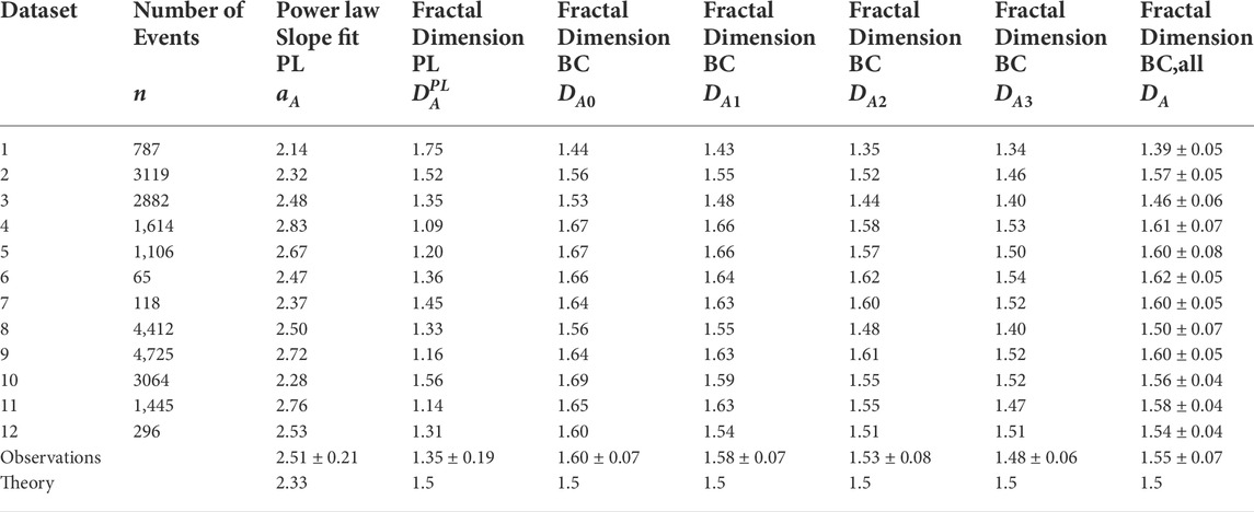
TABLE 1. Fractal Dimension obtained from power law slope fits (PL) and from the box counting (BC) method for 12 IRIS datasets.

The SOC-Inferred fractal dimension

The size distribution N(L) of length scales L, also called the scale-free probability conjecture (Aschwanden 2012; Aschwanden 2014), which essentially is the standard expression for the probability conservation in a power law distribution,

$N\left(L\right)dL\propto L^{-d}dL,(7)$

where d is the Euclidean space dimension, generally set to d = 3 for most real-world data. Note, that this occurrence frequency distribution function is simply a power law, which results from the reciprocal relationship of the number of events N(L) and the length scale L. Since the fractal dimension D_A for event areas A is defined as (Eq. 1),

$A=L^{D_A},(8)$

we obtain the inverse function L(A),

$L=A^{\left(1/D_A\right)},(9)$

and the derivative,

$\left(\frac{dL}{dA}\right)=A^{\left(1/D_A-1\right)},(10)$

so that we obtain the area distribution N(A) by substitution of L (Eq. 9) and the derivative dL/dA (Eq. 10) into N(L) (Eq. 7),

$N\left(A\right)dA=N\left[L\left(A\right)\right]\left(\frac{dL}{dA}\right)dA={\left[L\left(A\right)\right]}^{-d}{A}^{\left(1/D_A-1\right)}dA=A^{\left(-{\alpha }_A\right)}dA,(11)$

which yields the power law index α_A, for d = 3,

${\alpha }_A=1+\frac{\left(d-1\right)}{D_A}=1+\frac{2}{D_A}.(12)$

Vice versa we can then obtain the SOC fractal dimension D_A from an observed power law slope α_A (Table 1), by inverting α_A (D_A) in Eq. 12,

$D_A^{\mathit{SOC}}=\frac{2}{\left({\alpha }_A-1\right)}=\frac{3}{2}.(13)$

Using the theoretical value α_A = 7/3 ≈ 2.33 (Table 2), we expect a value of $D_A^{\mathit{SOC}}=1.5$ (Eq. 13), which is identical with the prediction of the mean Euclidean dimension $D_A^{ME}=1.5$ (Eq. 5) based on the mean of the extremal maximum and minimum values. This is an alternative method (Eq. 13) to calculate the fractal area dimension, in contrast to the mean Euclidean method (Eq. 5), which we call the SOC-inferred fractal dimension, because it uses the (power law) size distribution of areas that are defined in SOC models.

TABLE 2

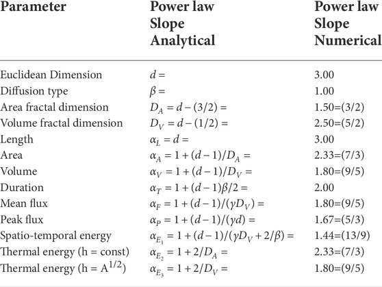
TABLE 2. Parameters of the standard SOC Model, with fractal dimensions D_x and power law slopes α_x of size distributions.

Observations

This is a follow-on study of previous work, “The power-law energy distributions of small-scale impulsive events on the active Sun: Results from IRIS” (Vilangot Nhalil et al., 2020). Although both studies use the same IRIS dataset, the former study (Vilangot Nhalil et al., 2020) analyzes the power law size distributions of event energies α_E, which is important for the assessment of coronal heating requirements, while the new study analyzes the fractal dimensions D_A of impulsive events, which allows us to discriminate different physical mechanisms from the photosphere up to the transition region and corona. We call these small-scale impulsive events simply “events”, which possibly could be related to “nanoflares” or “brightenings”. In the previous study, 12 IRIS datasets were investigated with an automated pattern recognition algorithm, yielding statistics of three parameters, namely the event area A (in units of pixels), the event (radiative) energy E (in units of erg), and event durations or lifetimes T (in units of seconds). IRIS has pixels with a size of 0.17′′ ≈ 0.123 Mm, which have been rebinned to L_pixel = 0.33′′ ≈ 0.247 Mm. The pixel size of areas thus corresponds to $A_{\mathit{pixel}}=L_{\mathit{pixel}}^2=0.247^2$ Mm² = 0.06076 Mm². The range of event areas covers A = 4–677 pixels, which amounts to length scales of $L=\sqrt{A}=(2-26)$ pixels, or L = (2–26)*0.247 Mm ≈ (0.5-6.4) Mm = (500-6400) km. The date of observations, the field-of-view (FOV), the cadence, and the NOAA active region numbers are listed in Table 1 of Vilangot Nhalil et al. (2020), for each of the 12 IRIS datasets.

The automated pattern recognition code was run with different threshold levels of 3, 5, and 7 σ in the previous event detection method of Vilangot Nhalil et al. (2020), from which we use the 3-σ level here. The values in Table 2 of the paper by Vilangot Nhalil et al. (2020) demonstrate that the fractal dimension is stable for different thresholds, as well as for noise filtering applied with diverse thresholds.

We use Slitjaw images (SJI) of the 1,400 Å channel of IRIS, which are dominated by the Si IV 1394 Å and 1,403 Å resonance lines, formed in the transition region. Vilangot Nhalil et al. (2020) compared also images from the SJI 1330 Å channel, which is dominated by the C II 1,335 Å and 1,336 Å lines, originating in the upper chromosphere and transition region at formation temperatures of T_e ≈ 3 × 10⁴ K and T_e ≈ 8 × 10⁴ K (Rathore and Carlsson 2015; Rathore et al., 2015).

Size distributions

Our first measurement is the fitting of a power law distribution function $N(A)\propto A^{-{\alpha }_A}$ of the event (or nanoflare) areas A, separately for each of the 12 IRIS datasets, as shown in Figure 1. The area of the event is a combination of all the spatially connected 3-σ pixels throughout their lifetime. The lowest bin was discarded in the histogram when a visible deviation from a power law was apparent. The number of events amounts to 23,633 for all 12 datasets together, varying from 65 to 4,725 events per IRIS dataset (Table 1). The power law slope fits vary from the lowest value α_A = 2.14 (dataset #1) to the highest value α_A = 2.83 (dataset #4), having a mean and standard deviation of (Figure 2, top panel).

$a_A^{\mathit{obs}}=2.51\pm 0.21.(14)$

The area size distributions are shown superimposed for the 12 IRIS datasets (Figure 2, top panel), which illustrates almost identical power law slopes in different IRIS datasets.

FIGURE 1

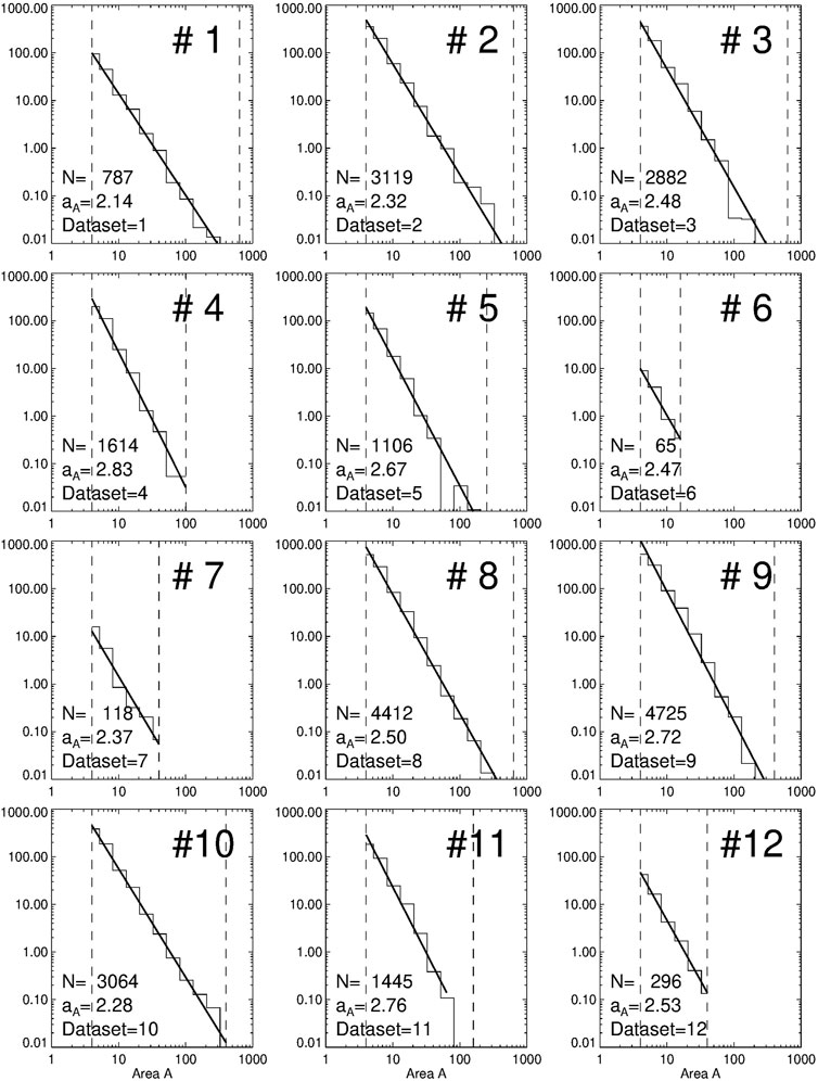
FIGURE 1. Size distributions of flare areas A for 12 datasets observed with IRIS SJI 1400 Å in different active regions.

FIGURE 2

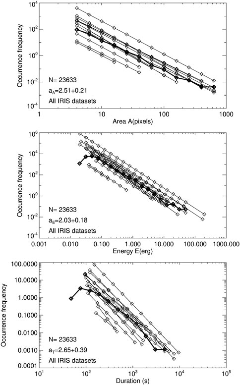
FIGURE 2. Power law fits to the size distributions of three SOC parameters: the event area A (top panel), the radiative energy E (middle panel), and the time duration (bottom panel). Individual fits to each of the 12 IRIS datasets are indicated with thin line style, while the fit to all events combined is indicated with thick line style, and the power law slopes are given in each panel.

Fitting the energy size distributions, $N(E)\propto E^{-{\alpha }_E}$, yields the following mean for all 12 IRIS datasets (Figure 2, middle panel),

$a_E^{\mathit{obs}}=2.03\pm 0.18.(15)$

Fitting the duration size distributions, $N(T)\propto T^{-{\alpha }_T}$, yields the following mean for all 12 IRIS datasets (Figure 2, bottom panel),

$a_T^{\mathit{obs}}=2.65\pm 0.39.(16)$

We will interpret these power law slopes in terms of SOC models in Size distributions.

The box-counting fractal dimension

The next parameter that we are interested in is the fractal dimension. A standard method to determine the fractal dimension D_A of an image is the box-counting method, which is defined by the asymptotic (L↦0) ratio of the fractal area A to the length scale L, i.e., D_A = log(A)/log(L), also called Hausdorff (fractal) dimension. We test the fractality by varying the pixel sizes (or spatial resolution) by powers of two, i.e., L_i = 2ⁱ = [1, 2, 4, 8] for i = [0, 1, 2, 3]. In order to normalize to the same number of events for each spatial resolution, the fractal (Hausdorff) dimension is defined by (e.g., Hirzberger et al., 1997),

$D_{A,i}=\frac{\log \left(A_i{2}^{2i}\right)}{\log \left(L_i{2}^i\right)},(17)$

where L_i is the observed length scale, and A_i is the observed fractal area, measured at different spatial resolutions. If the fractal dimension D_A,i stays more or less constant for different spatial resolutions L_i = [1, 2, 4, 8], then the dimension D_A,i is said to be “fractal”.

It has been pointed out that the detection of small-scale impulsive events requires a careful subtraction of event-unrelated background noise in the IRIS 1400 Å data (Vilangot Nhalil et al., 2020). The main effect of background subtraction is the related change in the fractal area, which causes a sensitive bias: If too much background is subtracted, the fractal area is smaller and the resulting fractal dimension is too small, and vice versa when the estimated background is under-estimated. At times and locations where no impulsive events occur, the flux distribution of an image shows a Gaussian distribution function (due to the random noise), while a heavy-tail occurs during active times (due to SOC-generated avalanches). In the case of a dominant noise component, a Gaussian can be fitted to the size distribution function, which yields a mean I_avg and a standard deviation I_sig. A 1-σ threshold can then be defined by,

$I_{\text{thr}}=I_{\text{avg}}+I_{\text{sig}}.(18)$

which separates the linear noise fluctuations (at I (x, y) ≤ I_thr) from the nonlinear avalanches (at I (x, y) ≥ I_thr). The calculation of a fractal dimension is then obtained from the ratio log (A_i2²ⁱ)/log (L_i2ⁱ) (Eq. 17), where the area A_i includes a count of all pixels with a flux value above the threshold, i.e., I (x, y) > I_thr, and the length scale L_i is the number of pixels that measure the length scale of a SOC avalanche.

We show the fractal dimensions measured with Eq. 17, for each of the 12 IRIS datasets and the 4 spatial resolutions D_A0, D_A1, D_A2, and D_A3 in Table 1, which reveal a very narrow spread of values D_A for the fractal dimension, with a mean and standard deviation of a few percents (Table 1),

$D_A^{\mathit{obs}}=1.55\pm 0.07.(19)$

Note, that the values obtained from different IRIS datasets and with different spatial resolutions are all consistent among each other and do not show any systematic dependency on the spatial resolution. Moreover, they are consistent with the theoretical expectation of the mean Euclidean dimension $D_A^{ME}$ (Eq. 5) and the SOC-Inferred value $D_A^{\mathit{SOC}}$ (Eq. 13),

$D_A^{ME}=D_A^{\mathit{SOC}}=\frac{3}{2}=1.5.(20)$

The fractal nature of the 12 IRIS datasets is rendered in Figure 3 and 4, where the black areas correspond to zones with enhanced emission, and the white areas correspond to the background with weak emission. The successive reduction of spatial resolution is shown in Figure 4.

FIGURE 3

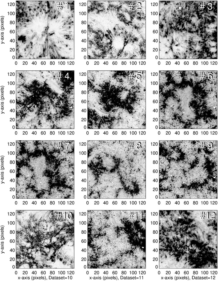
FIGURE 3. Intensity maps of 12 different active regions, observed with IRIS SJI 1400 Å. Black color indicates emission, and white color indicates the faint background.

FIGURE 4

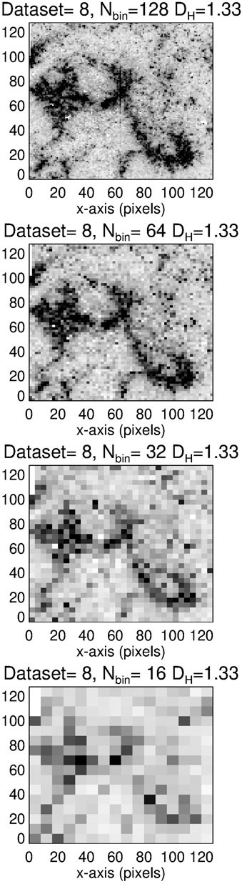
FIGURE 4. The IRIS dataset 8 is shown with different spatial resolutions of 128, 64, 32, and 16 bins, which demonstrates the scale-free definition of the Hausdorff dimension D_H = 1.33. Black color indicates emission, and white color indicates the faint background.

An example of a theoretical fractal pattern with a close ressemblance to the observed transition region patterns of dataset #8 is shown in Figure 5, which is called the “golden dragon fractal” and has a Hausdorff dimension of D_A = 1.61803.

FIGURE 5

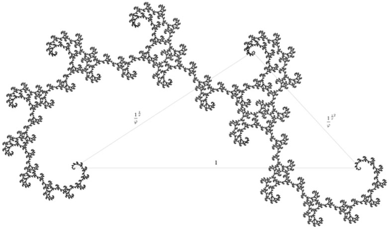
FIGURE 5. This numerically calculated fractal pattern is called a golden dragon and has a Hausdorff dimension of D_A = 1.61803. (https://en.wikipedia.org/wiki/List_of_fractals_by_Hausdorff_dimension). Note the similarity with dataset #8 in Figure 4.

Fractal dimensions across the solar atmosphere

In Table 3 we compile fractal dimensions obtained from photospheric, chromospheric, and transition region fractal features, which may be different from coronal and flare-like size distributions. The fractal dimension has been measured in photospheric wavelengths with the perimeter-area method, containing dominantly granules and super-granulation features (Roudier and Muller 1986; Hirzberger et al., 1997; Berrilli et al., 1998; Bovelet and Wiehr 2001; Paniveni et al., 2005, 2010), which exhibit a mean value of (Table 3),

$D_A^{\mathit{gran}}=1.23\pm 0.09.(21)$

Although this mean value is averaged from different solar features (granular cells and supergranular cells), as well as from different atmospheric heights (photospheric and chromospheric Ca II K data), the fractal dimension varies only by a small factor of ±7%. We have to be aware that photospheric emission originates from a lower altitude than any transition region or coronal feature. The relatively low value obtained for granulation features thus indicates that the granulation features seen in optical wavelengths are almost curvi-linear (with little area-filling topologies), which is expected for sparse photospheric mass flows along curvi-linear flow lines.

TABLE 3

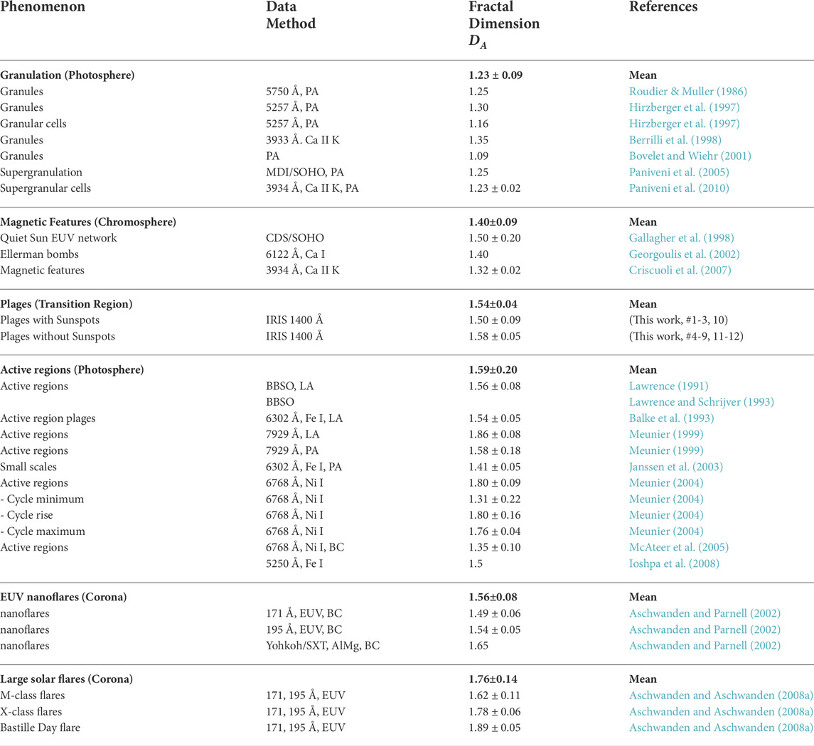
TABLE 3. The fractal dimensions of granules, plages, active regions, nanoflares, and large flares. Different methods are indicated with the acronyms (LA = Linear-area; PA = perimeter-area, and C = box counting. Mean values and standard deviations of each group are indicated with bold numbers. Studies based on the Ca II K line extend over both the photospheric and chromospheric zone.

A second feature we consider are plages in the transition region, measured with IRIS 1400 Å (Vilangot Nhalil et al., 2020), which have formation temperatures of $\approx 10^{3.7}-10^{5.2}$ K in the lower transition region, exhibiting a mean value of (Table 3),

$D_A^{\mathit{plage}}=1.54\pm 0.04.(22)$

A third feature is an active region, observed in photospheric magnetograms and analyzed with the linear-area method (Lawrence 1991; Balke et al., 1993; Lawrence and Schrijver 1993; Meunier 1999; Janssen et al., 2003; Meunier 2004; Ioshpa et al., 2008), or with the box-counting method (McAteer et al., 2005). The mean value of fractal dimensions measured in active regions is found to be (Table 3),

$D_A^{AR}=1.59\pm 0.20.(23)$

Apparently, active regions organize magnetic features into quasi-space-filling, area-like geometries.

Nanoflare events constitute a fourth phenomenon, which has been related to the SOC interpretation since Lu and Hamilton (1991). Nanoflares have been observed in EUV 171 Å and 195 Å with the TRACE instrument, as well as in soft X-rays using the Yohkoh/SXT (Solar X-Ray Telescope) (Aschwanden and Parnell 2002), which show a mean value of (see Table 3),

$D_A^{\mathit{nano}}=1.56\pm 0.08.(24)$

Nanoflares have been observed in the Quiet Sun and appear to have a similar fractal dimension as impulsive brightenings in active regions measured in magnetograms.

For completeness we list also the fractal dimension measured in large solar flares, for M-class flares, X-class flares, and the Bastille Day flare (Aschwanden and Aschwanden 2008a), as observed in the EUV, which all together exhibit a mean value of (Table 3),

$D_A^{\mathit{flare}}=1.76\pm 0.14.(25)$

This is the largest mean value of any measured fractal dimension, which indicates that the flare process fills the flare area almost completely, due to the superposition of many coronal postflare loops that become filled as a consequence of the chromospheric evaporation process.

Thus, we can distinguish four groups with significantly different fractal properties in photospheric, chromospheric, transition region, and coronal data (Table 4). A first group has a very low fractal dimension (D_A ≈ 1.2) that indicates curvi-linear features produced by super-granulation flows, a second group with chromospheric (network) features has a mean of (D_A ≈ 1.4), a third group with intermediate fractal dimensions (D_A ≈ 1.54) includes active region features in the photosphere, plages in the transition region, and EUV nanoflare events, and a fourth group with high values of fractal dimenions (D_A ≈ 1.8) that includes large (M- and X-class) flares, likely to be caused by area-like topologies of magnetic reconnection and chromospheric evaporation processes.

TABLE 4

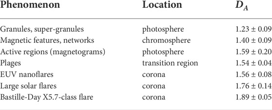
TABLE 4. Summary of solar phenomena, solar location, and range of fractal dimensions. Studies based on the Ca II K line cover both the photospheric and chromospheric zone.

Discussion

Basic fractal dimension measurement methods

A fractal geometry is a ratio that provides a statistical index of complexity, and changes as a function of a length scale that is used as a yardstick to measure it (Mandelbrot 1977). There are four integer values of Euclidean dimensions d = [0, 1, 2, 3]: zero-dimensional point-like structures (d = 0), one-dimensional linear or curvi-linear structures (d = 1), two-dimensional area-like structures (d = 2), and three-dimensional voluminous structures (d = 3). All other values between 0 and 3 are non-integer Euclidean dimensions and are called fractal dimensions.

Basic methods to measure fractal dimensions include the linear-area (LA) method, the perimeter-area (PA) method, and the box-counting (BC) method. The LA method calculates the ratio of a fractal area A to a quasi-space-filled (encompassing) quadratic area with size L². Similarly, the PA method yields a ratio of the encompassing curve length or perimeter length (P = πr in the case of a circular boundary). The box-counting method uses a cartesian (2-D or 3-D) lattice grid [x, y] and counts all pixels above some threshold or background, and takes the ratio to the total counts of all pixels inside the encompassing coordinate grid. These three methods appear to be very simple, but are not unique. The resulting fractal dimensions may depend on the assumed level of background subtraction, or on the spatial resolution, if not properly normalized. The encompassing perimeter depends on the definition of the perimeter (square, circle, polygon, etc.). Multiple different geometric patterns may cause a variation of the fractal dimension across an image or data cube. Temporal variability can modulate the fractal dimension as a function of time. Detailed discussions and examples of the topics of the background subtraction, the spatial resolution, the selection of the field-of-view, and the temporal stability are discussed in almost all references that are listed in Table 3. The detailed incorporation of a fractal measurement method differs in each study.

Theoretical values of fractal dimensions converge by definition to a unique value (e.g., D_A = 1.61803 for the golden dragon fractal, Figure 5), while observed data almost always exhibit some spatial inhomogeneity that gives rise to a spread of fractal dimension values across an image.

Granulation in photosphere

A compilation of fractal dimensions measured in photospheric, chromospheric, and coronal wavelengths is given in Table 3. The solar granulation has a typical spatial scale of L = 1,000 km, or a perimeter of P = πL ≈ 3000 km. Roudier and Muller (1986) measured the areas A and perimeters P of 315 granules and found a power law relation P ∝ A^D/2, with D = 1.25 for small granules (with perimeters of p ≈ 500–4,500 km) and D = 2.15 for large granules (with p = 4,500–15, 000 km). The smaller granules were interpreted in terms of turbulent origin, because the predicted fractal dimension of an isobaric atmosphere with isotropic and homogeneous turbulence is D = 4/3 ≈ 1.33 (Mandelbrot 1977). Similar values (D_A = 1.30 and D_A = 1.16) were found by Hirzberger et al. (1997), Ermolli et al. (1998), and Berrilli et al. (1998). Bovelet and Wiehr (2001) tested different pattern recognition algorithms (Fourier-based recognition technique FBR and multiple-level tracking MLT) and found that the value of the fractal dimension strongly depends on the measurement method. The MLT method yielded a fractal dimension of D_A = 1.09, independent of the spatial resolution, the heliocentric angle, and the definition in terms of temperature or velocity. Paniveni et al. (2005) found a fractal dimension of D_A ≈ 1.25 and concluded, by relating it to the variations of kinetic energy, temperature, and pressure, that the super-granular network is close to being isobaric and possibly of turbulent origin. Paniveni et al. (2010) investigated super-granular cells and found a fractal dimension of D_A = 1.12 for active region cells, and D_A = 1.25 for quiet region cells, a difference that they attributed to the inhibiting effect of the stronger magnetic field in active regions. Averaging all fractal dimensions related to granular datasets we obtain a mean value of D_A = 1.23 ± 0.09, which is closer to a curvi-linear topology (D_A ≳ 1.0) than to an area-filled geometry (D_A ≲ 2.0).

The physical understanding of solar (or stellar) granulation has been advanced by numerical magneto-convection models and N-body dynamic simulations, which predict the evolution of small-scale (granules) into large-scale features (meso- or super-granulation), organized by surface flows that sweep up small-scale structures and form clusters of recurrent and stable granular features (Hathaway et al., 2000; Berrilli et al., 2005; Rieutord et al., 2008; Rieutord et al., 2010).

The fractal multi-scale dynamics has been found to be operational in the quiet photosphere, in a quiescent non-flaring state, as well as during flares (Uritsky and Davila 2012).

The fractal structure of the solar granulation is obviously a self-organizing pattern that is created by a combination of subphotospheric magneto-convection and surface flows, which are turbulence-type phenomena.

Transition region

Measurements of the fractal dimension and power law slope of the size distribution in the transition region have been accomplished with IRIS 1400 Å observations of plages and sunspot regions (Vilangot Nhalil et al., 2020; and this work, see Table 3). Fractal dimensions of transition region features were evaluated with a box-counting method here, yielding a range of D_A ≈ 1.54 ± 0.04 for the 12 datasets of plages in the transition region listed in Tables 1 and 3. The structures observed in the 1,400 Å channel of IRIS are dominated by the Si IV 1394 Å and 1,403 Å resonance lines, which are formed in the transition region temperature range of T = 10^4.5–10⁶ K, sandwiched between the cooler chromosphere and the hotter corona. Apparently, the fractal dimension is not much different in plages with sunspots (D_A = 1.58 ± 0.05), or in field-of-views without sunspots (D_A = 1.52 ± 0.09), (Table 3).

One prominent feature in the transition region is the phenomenon of “moss”, which appears as a bright, dynamic pattern with dark inclusions, on spatial scales of L ≈ 1–3 Mm, which has been interpreted as the upper transition region above active region plages and below relatively hot loops (De Pontieu et al., 1999). Besides transition region features, measurements in chromospheric (Quiet-Sun) network structures in the temperature range of T = 10^4.5–10⁶ K yield fractal dimensions of D_A = 1.30–1.70 (Gallagher et al., 1998). Furthermore, a value of D_A ≈ 1.4 was found for so-called Ellerman bombs (Georgoulis et al., 2002), which are short-lived brightenings seen in the wings of the Hα line from the low chromosphere. In addition, a range of D_A ≈ 1.25–1.45 was measured from a large survey of 9342 active region magnetograms (McAteer et al., 2005). Measurements of SOHO/CDS in EUV lines in the temperature range of T_e ≈ 10^4.5–10⁶ revealed a distinct temperature dependence: fractal dimensions of D_A ≈ 1.5–1.6 were identified in He I, He II, OIII, OIV, OV, Ne VI lines at log (T_e) ≈ 5.8, then a peak with D_A ≈ 1.6–1.7 at log (T_e) ≈ 5.9, and a drop of D_A ≈ 1.3–1.35 at log (T_e) ≈ 6.0 (see Figure 11 in Gallagher et al., 1998). The temperature dependence of the fractal dimension can be interpreted in terms of sparse heating that produces curvi-linear flow patterns with low fractal dimensions of D_A ≲ 1.5, while strong heating produces volume-filling by chromospheric evaporation with high fractal dimensions D_A ≳ 1.5.

In recent work it was found that the concept of mono-fractals has to be generalized to multi-fractals to quantify the spatial structure of solar magnetograms more accurately (Lawrence and Schrijver 1993; Cadavid et al., 1994; Lawrence et al., 1996; McAteer et al., 2005; Conlon et al., 2008; Giorgi et al., 2015).

Photospheric magnetic field in active regions

A number of studies investigated the fractal dimension of the photospheric magnetic field, as observed in magnetograms in the Fe I (6,302 Å, 5,250 Å) or Ni I (6,768 Å) lines. Meunier (1999) evaluated the fractal dimension with the perimeter-area method and found D_A = 1.58 for super-granular structures to D_A = 1.58 for the largest structures, while the linear size-area method yielded D_A = 1.78 and D_A = 1.94, respectively. In addition, a solar cycle dependence was found by Meunier (2004), with the fractal dimension varying from D_A = 1.09 ± 0.11 (minimum) to D_A = 1.73 ± 0.01 for weak-field regions (B_m < 900 G), and D_A = 1.53 ± 0.06 (minimum) to D_A = 1.80 ± 0.01 for strong-field regions (B_m > 900 G), respectively. A fractal dimension of D_A = 1.41 ± 0.05 was found by Janssen et al. (2003), but the value varies as a function of the center-to-limb angle and is different for a speckle-reconstructed image that eliminates seeing and noise.

A completely different approach to measure the fractal dimension D was pursued in terms of a 2-D diffusion process, finding fractal diffusion with dimensions in the range of D ≈ 1.3–1.8 (Lawrence 1991) or D = 1.56 ± 0.08 (Lawrence and Schrijver 1993) by measuring the dependence of the mean square displacement of magnetic elements as a function of time. Similar results were found by Balke et al. (1993). The results exclude Euclidean 2-D diffusion but are consistent with percolation theory for diffusion of clusters at a density below the percolation threshold (Balke et al., 1993; Lawrence and Schrijver 1993).

Other methods to analyze fractals in the photospheric magnetic field in active regions focus on the scaling behavior of the structure function, applied to the longitudinal magnetic field (Abramenko et al., 2002), which can discriminate between weak and fully developed turbulence. Both SOC and intermittent turbulence (IT) appear to co-exist in the solar corona, since power-law avalanche statistics as well as multi-scaling of structure functions are observed simulaneously (Uritsky et al., 2007). Moreover, stochastic coupling between the solar photopshere and the corona indicate an intimate spatial connection (Uritsky et al., 2013).

Coronal flares

Although this study is focused on the fractal geometry of transition region features observed with IRIS, we compare these results also with coronal values. The fractal dimension of coronal events has been measured for 10 X-class flares, 10 M-class flares, and the Bastille-Day flare (Aschwanden and Aschwanden 2008a; Aschwanden and Aschwanden 2008b). Interestingly, these datasets exhibit relatively large values of the fractal dimension, with a mean and standard deviation of D_A = 1.76 ± 0.14. They show a trend that the largest flares, especially X-class flares, exhibit the highest values of D_A ≲ 1.8–1.9 (Table 3). If we attribute flare events to the magnetic reconnection process, the observations imply that the flare plasma fills up the flare volume with a high space-filling factor, which is consistent with the chromospheric evaporation process.

Phenomena of smaller magnitude than large flares include microflares, nanoflares, coronal EUV brightenings, etc. Such small-scale variability events are found to have a mean fractal dimension of D_A = 1.56 ± 0.08 (Table 3), which is compatible with those found in M-class flares, but clearly has a lower fractal dimension than large flares, i.e., D_A = 1.76 ± 0.14 (Table 3).

Self-organized criticality models

The generation of magnetic structures that bubble up from the solar convection zone to the solar surface by buoyancy, observed as emerging flux phenomena in form of active regions, sunspots, and pores, can be statistically described as a random process, self-organization with (SOC) and without (SO) criticality, percolation, or a diffusion process. Random processes produce incoherent structures, in contrast to the coherent magnetic flux concentrations observed in sunspots. A self-organization (SO) process needs a driving force and a counter-acting feedback mechanism that produces ordered structures (such as the convective granulation cells; Aschwanden et al., 2018). A SOC process exhibits power law size distributions of avalanche sizes and durations. The finding of a fractal dimension of a power law size distribution in magnetic features alone is not a sufficient condition to prove or rule out any of these processes. Nevertheless, the fractal dimension yields a scaling law between areas ($A\propto L^{D_2}$) or volumes ($V\propto L^{D_3}$), and length scales L that quantify scale-free (fractal) processes in form of power laws and can straightforwardly be incorporated in SOC-like models.

If we compare the standard SOC parameters measured in observations (Figure 2) with the theoretically expected values from the standard SOC model (Table 2), we find that the power law slopes for event areas A agree well $(a_A^{\mathit{obs}}=2.51\pm 0.21)$ versus $a_A^{\mathit{theo}}=2.33$ (Figure 2), while the power law slopes for the radiated energy E agree within the stated uncertainties, $(a_E^{\mathit{obs}}=2.03\pm 0.18)$ versus $a_E^{\mathit{theo}}=1.80$ (Figure 2), but the power law slopes for the time duration T disagree $(a_T^{\mathit{obs}}=2.65\pm 0.39)$ versus $a_T^{\mathit{theo}}=2.00$ (Figure 2). The latter disagreement is possibly caused by the restriction of a constant minimum event lifetime (either 60 s or 110 s) that was assumed in the previous work (Vilangot Nhalil et al., 2020). The interpretation of these results implies that transition region brightenings have a similar statistics as the SOC model, at least for active regions, nanoflares, and large flares, with a typical fractal dimension of D_A ≈ 1.54 ± 0.04, but are significantly lower for photospheric granulation (D_A ≈ 1.23 ± 0.09), which implies the dominance of sparse quasi-linear flow structures in the photosphere and transition region.

Conclusion

Our aim is to obtain an improved undestanding of fractal dimensions and size distributions observed in the solar photosphere and transition region, which complement previous measurements of coronal phenomena, from nanoflares to the largest solar flares. Building on the previous study “Power-law energy distributions of small-scale impulsive events on the active Sun: Results from IRIS”, we are using the same IRIS 1,400 Å data, extracted with an automated pattern recognition code during 12 time episodes observed in plage and sunspot regions. A total of 23,633 events has been obtained, quantified in terms of event areas A, radiative energies E, and event durations T. The results can be summarized as follows:

1. Fractal dimensions, measured in solar images at various wavelengths and spatial resolutions, cover a range of D_A = 1–2. We can organize the 7 types of solar phenomena and their range of fractal dimensions in Table 4, which can be subdivided into 4 non-overlapping groups: Granules and super-granules have a fractal dimension of (D_A ≈ 1.2), chromospheric magnetic features and networks have a fractal dimension of (D_A ≈ 1.4), active regions, plages, and coronal nanoflares have a mean fractal dimension of (D_A ≈ 1.5), and large flares have the highest range (D_A ≈ 1.8). Low values of the fractal dimension (D_A ≈ 1) are consistent with curvi-linear flow patterns, while large values are consistent with space-filling features produced by chromospheric evaporation in large flares. A mean value D_A ≈ 1.5 has been found to represent a useful approximation in standard SOC models.

2. We calculate a power law fit to the size distribution $N(A)\propto A^{-{\alpha }_A}$ of event areas A, and find a mean value of a_A = 2.51 ± 0.21 that agrees well with the value a_A = 2.33 expected from the theoretical SOC model. Consequently, brightenings in plages of the transition region are consistent with generic SOC avalanches.

3. Based on the power law slope αA we derive the fractal dimension $D_A^{PL}=2/({\alpha }_A-1)$, which yields a mean observed value of $D_A^{PL}=1.35\pm 0.19$ and approximately matches the theoretial mean value of D_A = 1.5. Alternatively, we obtain with the standard box-counting method an observed value of D_A = 1.54 ± 0.04.

4. Synthesizing the measurements of the fractal dimension from photospheric, chromospheric, transition region, and coronal data we arrive at 7 groups that yield the following means and standard deviations of their fractal dimension: From these 7 groups we can discriminate four (Table 4) non-overlapping ranges with significantly different fractal dimensions, which imply different physical mechanisms: Low values of the fractal dimension (D_A ≈ 1.2) indicate curvi-linear granulation flows; larger values (D_A ≈ 1.4) align fractal structures with chromospheric network cells; intermediate values of (D_A ≈ 1.54) are characteristic for brightening events in the Quiet Sun and transition region; while large values (D_A ≲ 2.0) are consistent with quasi-space-filling features produced by chromospheric evaporation in large flares.

The analysis presented here demonstrates that we can distinguish between (i) physical processes with sparse curvi-linear flows, as they occur in granulation, meso-granulation, and super-granulation, and (ii) physical processes with quasi-space-filling flows, as they occur in the chromospheric evaporation process during solar flares. IRIS data can therefore be used to diagnose mass flows in the transition region. Moreover, reliable measurements of the fractal dimension yields realistic plasma filling factors that are important in the estimate of radiative energies and hot plasma emission measures. Future work on fractal dimensions in multi-wavelength datasets from IRIS and AIA/SDO may clarify the dynamics of coronal heating events.

Data availability statement

The raw data supporting the conclusion of this article will be made available by the authors, without undue reservation.

Author contributions

All authors listed have made a substantial, direct, and intellectual contribution to the work and approved it for publication.

Funding

This work was partially supported by NASA contract NNX11A099G “Self-organized criticality in solar physics”, NASA contract NNG04EA00C of the SDO/AIA instrument, and the IRIS contract NNG09FA40C to LMSAL.

Acknowledgments

We acknowledge constructive comments of an reviewer and stimulating discussions (in alphabetical order) with Sandra Chapman, Paul Charbonneau, Henrik Jeldtoft Jensen, Adam Kowalski, Alexander Milovanov, Leonty Miroshnichenko, Jens Juul Rasmussen, Karel Schrijver, Vadim Uritsky, Loukas Vlahos, and Nick Watkins.

Conflict of interest

The authors declare that the research was conducted in the absence of any commercial or financial relationships that could be construed as a potential conflict of interest.

Publisher’s note

All claims expressed in this article are solely those of the authors and do not necessarily represent those of their affiliated organizations, or those of the publisher, the editors and the reviewers. Any product that may be evaluated in this article, or claim that may be made by its manufacturer, is not guaranteed or endorsed by the publisher.

References

Abramenko, V. I., Yurchyshyn, V. B., Wang, H., Spirock, T. J., and Goode, P. R. (2002). Scaling behavior of structure functions of the longitudinal magnetic field in active regions on the Sun. ApJ 577, 487. doi:10.1086/342169

CrossRef Full Text | Google Scholar

Aschwanden, M. J. (2014). A macroscopic description of self-organized systems and astrophysical applications. Astrophys. J. 782, 54. doi:10.1088/0004-637x/782/1/54

CrossRef Full Text | Google Scholar

Aschwanden, M. J. (2012). A statistical fractal-diffusive avalanche model of a slowly-driven self-organized criticality system. Astron. Astrophys. 539, A2. doi:10.1051/0004-6361/201118237

CrossRef Full Text | Google Scholar

Aschwanden, M. J., and Aschwanden, P. D. (2008b). Solar flare geometries: II. The volume fractal dimension. Astrophys. J. 574, 544–553. doi:10.1086/524370

CrossRef Full Text | Google Scholar

Aschwanden, M. J., and Aschwanden, P. D. (2008a). Solar flare geometries: I. The area fractal dimension. Astrophys. J. 574, 530–543. doi:10.1086/524371

CrossRef Full Text | Google Scholar

Aschwanden, M. J., Crosby, N., Dimitropoulou, M., Georgoulis, M. K., Hergarten, S., McAteer, J., et al. (2016). 25 Years of self-organized criticality: Solar and astrophysics. Space Sci. Rev. 198, 47–166. doi:10.1007/s11214-014-0054-6

CrossRef Full Text | Google Scholar

Aschwanden, M. J., and Parnell, C. E. (2002). Nanoflare statistics from first principles: Fractal geometry and temperature synthesis. Astrophys. J. 572, 1048.

CrossRef Full Text | Google Scholar

Aschwanden, M. J. (2022b). Reconciling power-law slopes in solar flare and nanoflare size distributions. Astrophys. J. Lett. 934, L3. doi:10.3847/2041-8213/ac7b8d

CrossRef Full Text | Google Scholar

Aschwanden, M. J., Scholkmann, F., Bethune, W., Schmutz, W., Abramenko, W., Cheung, M. C. M., et al. (2018). Order out of randomness: Self-organization processes in astrophysics. Space Sci. Rev. 214, 55. doi:10.1007/s11214-018-0489-2

CrossRef Full Text | Google Scholar

Aschwanden, M. J. (2011). Self-organized criticality in Astrophysics: The statistics of nonlinear processes in the universe. New York: Springer-Praxis, 416. ISBN 978-3-642-15000-5.

Google Scholar

Aschwanden, M. J. (2022a). The fractality and size distributions of astrophysical self-organized criticality systems. Astrophys. J. 934, 33. doi:10.3847/1538-4357/ac6bf2

CrossRef Full Text | Google Scholar

Bak, P. (1996). How nature works: The science of self-organized criticality. New York: Copernicus.

Google Scholar

Bak, P., Tang, C., and Wiesenfeld, K. (1988). Self-organized criticality. Phys. Rev. A . 38 (1), 364–374. doi:10.1103/physreva.38.364

PubMed Abstract | CrossRef Full Text | Google Scholar

Bak, P., Tang, C., and Wiesenfeld, K. (1987). Self-organized criticality: An explanation of the 1/fnoise. Phys. Rev. Lett. 59 (27), 381–384. doi:10.1103/physrevlett.59.381

PubMed Abstract | CrossRef Full Text | Google Scholar

Balke, A. C., Schrijver, C. J., Zwaan, C., and Tarbell, T. D. (1993). Percolation theory and the geometry of photospheric magnetic flux concentrations. Sol. Phys. 143, 215–227. doi:10.1007/bf00646483

CrossRef Full Text | Google Scholar

Berrilli, F., Del Moro, D., Russo, S., Consolini, G., and Straus, T. (2005). Spatial clustering of photospheric structures. Astrophys. J. 632, 677–683. doi:10.1086/432708

CrossRef Full Text | Google Scholar

Berrilli, F., Florio, A., and Ermolli, I. (1998). On the geometrical properties of the chromospheric network. Sol. Phys. 180, 29–45. doi:10.1023/a:1005023819431

CrossRef Full Text | Google Scholar

Bovelet, B., and Wiehr, E. (2001). A new algorithm for pattern recognition and its application to granulation and limb faculae. Sol. Phys. 201, 13–26. doi:10.1023/a:1010344827952

CrossRef Full Text | Google Scholar

Cadavid, A. C., Lawrence, J. K., Ruzmaikin, A., and Kayleng-Knight, A. (1994). Multifractal models of small-scale solar magnetic fields. Astrophys. J. 429, 391. doi:10.1086/174329

CrossRef Full Text | Google Scholar

Conlon, P. A., Gallagher, P. T., McAteer, R. T. J., Ireland, J., Young, C. A., Kestener, P., et al. (2008). Multifractal properties of evolving active regions. Sol. Phys. 248, 297–309. doi:10.1007/s11207-007-9074-7

CrossRef Full Text | Google Scholar

Consolini, G., Carbone, V., Berrilli, F., Bruno, R., Bavassano, B., Briand, C., et al. (1999). Scaling behavior of the vertical velocity field in the solar photosphere. A&A 344, L33–L36.

Google Scholar

Criscuoli, S., Rast, M. P., Ermolli, I., and Centrone, M. (2007). On the reliability of the fractal dimension measure of solar magnetic features and on its variation with solar activity. Astron. Astrophys. 461, 331–338. doi:10.1051/0004-6361:20065951

CrossRef Full Text | Google Scholar

De Pontieu, B., Berger, T. E., Schrijver, C. J., and Title, A. M. (1999). Dynamics of transition region ’moss’ at high time resolution. Sol. Phys. 190, 419–435. doi:10.1023/a:1005220606223

CrossRef Full Text | Google Scholar

De Pontieu, B., Title, A. M., Lemen, J. R., Kushner, G. D., Akin, D. J., Allard, B., et al. (2014). The Interface region imaging Spectrograph (IRIS). Sol. Phys. 289, 2733. doi:10.1007/s11207-014-0485-y

CrossRef Full Text | Google Scholar

Ermolli, I., Fovi, M., Bernacchia, C., Berilli, F., Caccin, B., Egidi, A., et al. (1998). The prototype RISE-PSPT instrument operating in Rome. Sol. Phys. 177/1-2, 1–10.

CrossRef Full Text | Google Scholar

Ermolli, I., Giorgi, F., Romano, P., Zuccarello, F., Criscuoli, S., and Stangalini, M. (2014). Fractal and multifractal properties of active regions as flare precursors: A case study based on SOHO/MDI and SDO/HMI observations. Sol. Phys. 289, 2525–2545. doi:10.1007/s11207-014-0500-3

CrossRef Full Text | Google Scholar

Gallagher, P. T., Phillips, K. J. H., Harra-Murnion, L. K., and Keenan, F. P. (1998). Properties of the quiet Sun EUV network. A&A 335, 733.

Google Scholar

Georgoulis, M. K., Rust, D. M., Bernasconi, P. N., and Schmieder, B. (2002). Statistics, morphology, and energetics of Ellerman bombs. Astrophys. J. 575, 506–528. doi:10.1086/341195

CrossRef Full Text | Google Scholar

Giorgi, F., Ermolli, I., Romano, P., Stangalini, M., Zuccarello, F., and Criscuoli, S. (2015). The signature of flare activity in multifractal measurements of active regions observed by SDO/HMI. Sol. Phys. 290, 507–525. doi:10.1007/s11207-014-0609-4

CrossRef Full Text | Google Scholar

Hathaway, D. H., Beck, J. G., Bogart, R. S., Bachmann, K., Khatri, G., Petitto, J., et al. (2000). Sol. Phys. 193, 299–312. doi:10.1023/a:1005200809766

CrossRef Full Text

Hirzberger, J., Vazquez, M., Bonet, J. A., Hanslmeier, A., and Sobotka, M. (1997). Time series of solar granulation images. I. Differences between small and large granules in quiet regions. Astrophys. J. 480, 406–419. doi:10.1086/303951

CrossRef Full Text | Google Scholar

Ioshpa, B. A., Obridko, V. N., and Rudenchik, E. A. (2008). Fractal properties of solar magnetic fields. Astron. Lett. 34, 210–216. doi:10.1134/s1063773708030080

CrossRef Full Text | Google Scholar

Janssen, K., Voegler, A., and Kneer, F. (2003). On the fractal dimension of small-scale magnetic structures in the Sun. Astron. Astrophys. 409, 1127–1134. doi:10.1051/0004-6361:20031168

CrossRef Full Text | Google Scholar

Lawrence, J. K., Cadavid, A., and Ruzmaikin, A. (1996). On the multifractal distribution of solar magnetic fields. Astrophys. J. 465, 425. doi:10.1086/177430

CrossRef Full Text | Google Scholar

Lawrence, J. K. (1991). Diffusion of magnetic flux elements on a fractal geometry. Sol. Phys. 135, 249–259. doi:10.1007/bf00147499

CrossRef Full Text | Google Scholar

Lawrence, J. K., and Schrijver, C. J. (1993). Anomalous diffusion of magnetic elements across the solar surface. Astrophys. J. 411, 402. doi:10.1086/172841

CrossRef Full Text | Google Scholar

Lu, E. T., and Hamilton, R. J. (1991). Avalanches and the distribution of solar flares. Astrophys. J. 380, L89. doi:10.1086/186180

CrossRef Full Text | Google Scholar

Mandelbrot, B. B. (1977). The fractal geometry of nature. New York: W.H.Freeman and Company.

Google Scholar

McAteer, R. T. J., Aschwanden, M. J., Dimitropoulou, M., Georgoulis, M. K., Pruessner, G., Morales, L., et al. (2016). 25 Years of self-organized criticality: Numerical detection methods. Space Sci. Rev. 198, 217–266. doi:10.1007/s11214-015-0158-7

CrossRef Full Text | Google Scholar

McAteer, R. T. J., Gallagher, P. T., and Ireland, J. (2005). Statistics of active region complexity: A large-scale fractal dimension survey. Astrophys. J. 631, 628–635. doi:10.1086/432412

CrossRef Full Text | Google Scholar

Meunier, N. (2004). Complexity of magnetic structures: Flares and cycle phase dependence. Astron. Astrophys. 420, 333–342. doi:10.1051/0004-6361:20034044

CrossRef Full Text | Google Scholar

Meunier, N. (1999). Fractal analysis of michelson Doppler imager magnetograms: A contribution to the study of the formation of solar active regions. Astrophys. J. 515, 801–811. doi:10.1086/307050

CrossRef Full Text | Google Scholar

Paniveni, U., Krishan, V., Singh, J., and Srikanth, R. (2010). Activity dependence of solar supergranular fractal dimension. Mon. Not. R. Astron. Soc. 402 (1), 424–428. doi:10.1111/j.1365-2966.2009.15889.x

CrossRef Full Text | Google Scholar

Paniveni, U., Krishan, V., Singh, J., and Srikanth, R. (2005). On the fractal structure of solar supergranulation. Sol. Phys. 231, 1–10. doi:10.1007/s11207-005-1591-7

CrossRef Full Text | Google Scholar

Pruessner, G. (2012). Self-organised criticality. Theory, models and characterisation. Cambridge: Cambridge University Press.

Google Scholar

Rathore, B., Carlsson, M., and Leenaarts, J. (2015). The formation of irisdiagnostics. VI. The diagnostic potential of the C II lines at 133.5 nm in the solar atmosphere. Astrophys. J. 811, 81. doi:10.1088/0004-637x/811/2/81

CrossRef Full Text | Google Scholar

Rathore, B., and Carlsson, M. (2015). The formation of irisdiagnostics. V. A quintessential model atom of C II and general formation properties of the C II lines at 133.5 nm. Astrophys. J. 811, 80. doi:10.1088/0004-637x/811/2/80

CrossRef Full Text | Google Scholar

Rieutord, M., Meunier, N., Roudier, T., Rondi, S., Beigbeder, F., and Pares, L. (2008). Solar supergranulation revealed by granule tracking. Astron. Astrophys. 479, L17–L20. doi:10.1051/0004-6361:20079077

CrossRef Full Text | Google Scholar

Rieutord, M., Roudier, T., Rincon, F., Malherbe, J. M., Meunier, N., Berger, T., et al. (2010). On the power spectrum of solar surface flows. Astron. Astrophys. 512, A4. doi:10.1051/0004-6361/200913303

CrossRef Full Text | Google Scholar

Roudier, T., and Muller, R. (1986). Structure of the solar granulation. Sol. Phys. 107, 11–26. doi:10.1007/bf00155337

CrossRef Full Text | Google Scholar

Sharma, A. S., Aschwanden, M. J., Crosby, N. B., Klimas, A. J., Milovanov, A. V., Morales, L., et al. (2016). 25 Years of self-organized criticality: Space and laboratory plasmas. Space Sci. Rev. 198, 167–216. doi:10.1007/s11214-015-0225-0

CrossRef Full Text | Google Scholar

Uritsky, V. M., and Davila, J. M. (2012). Multiscale dynamics of solar magnetic structures. Astrophys. J. 748, 60. doi:10.1088/0004-637x/748/1/60

CrossRef Full Text | Google Scholar

Uritsky, V. M., Davila, J. M., Ofman, L., and Coyner, A. J. (2013). Stochastic coupling of solar photosphere and corona. Astrophys. J. 769, 62. doi:10.1088/0004-637x/769/1/62

CrossRef Full Text | Google Scholar

Uritsky, V. M., Paczuski, M., Davila, J. M., and Jones, S. I. (2007). Coexistence of self-organized criticality and intermittent turbulence in the solar corona. Phys. Rev. Lett. 99 (2), 025001. doi:10.1103/physrevlett.99.025001

PubMed Abstract | CrossRef Full Text | Google Scholar

Vilangot Nhalil, N. V., Nelson, C. J., Mathioudakis, M., Doyle, G. J., and Ramsay, G. (2020). Power-law energy distributions of small-scale impulsive events on the active Sun: Results from IRIS. Mon. Not. R. Astron. Soc. 499, 1385–1394. doi:10.1093/mnras/staa2897

CrossRef Full Text | Google Scholar

Watkins, N. W., Pruessner, G., Chapman, S. C., Crosby, N. B., and Jensen, H. J. (2016). 25 Years of self-organized criticality: Concepts and controversies. Space Sci. Rev. 198, 3–44. doi:10.1007/s11214-015-0155-x

CrossRef Full Text | Google Scholar