 Hongyang Zhou1*
 Lucile Turc1
 Yann Pfau-Kempf1
 Markus Battarbee1
 Vertti Tarvus1Maxime Dubart1
 Harriet George1Giulia Cozzani1
 Maxime Grandin1
 Urs Ganse1Markku Alho1Andreas Johlander2Jonas Suni1Maarja Bussov1Konstantinos Papadakis1Konstantinos Horaites1Ivan Zaitsev1
 Fasil Tesema1Evgeny Gordeev1
 Minna Palmroth 1,3
- 1University of Helsinki, Helsinki, Finland
- 2Swedish Institute of Space Physics, Uppsala, Sweden
- 3Finnish Meteorological Institute, Helsinki, Finland
Ultra-low frequency (ULF) waves are routinely observed in Earth’s dayside magnetosphere. Here we investigate the influence of externally-driven density variations in the near-Earth space in the ULF regime using global 2D simulations performed with the hybrid-Vlasov model Vlasiator. With the new time-varying boundary setup, we introduce a monochromatic Pc5 range periodic density variation in the solar wind. A breathing motion of the magnetopause and changes in the bow shock standoff position are caused by the density variation, the time lag between which is found to be consistent with propagation at fast magnetohydrodynamic speed. The oscillations also create large-scale stripes of variations in the magnetosheath and modulate the mirror and electromagnetic ion cyclotron modes. We characterize the spatial-temporal properties of ULF waves at different phases of the variation. Less prominent EMIC and mirror mode wave activities near the center of magnetosheath are observed with decreasing upstream Mach number. The EMIC wave occurrence is strongly related to pressure anisotropy and β‖, both vary as a function of the upstream conditions, whereas the mirror mode occurrence is highly influenced by fast waves generated from upstream density variations.
1 Introduction
The terrestrial magnetosphere contains a rich variety of low-frequency fluctuations. Magnetospheric ultra-low frequency (ULF) waves are categorized by continuous pulsations in five consecutive ranges 1–5 (Jacobs et al., 1964). ULF waves in the Pc5 range 150–600 s play a key role in the dynamics of Earth’s magnetosphere, in particular through their interaction with radiation belt electrons (Elkington, 2006; Zong et al., 2017; Ripoll et al., 2020), modulation of particle precipitation (Wang et al., 2020), total electron content (Kozyreva et al., 2020), geomagnetically induced currents (Heyns et al., 2021) and contribution to magnetosphere-ionosphere coupling via Joule heating and/or ion frictional heating with neutrals (Hartinger et al., 2015; Baddeley et al., 2017).
One important source of magnetospheric Pc5 waves are fluctuations of the upstream solar wind parameters in the same frequency range, e.g. Kessel (2008); Viall et al. (2009); Zong et al. (2017). Pressure variations in the solar wind can trigger fast shock and fast rarefaction waves downstream of the bow shock (Wu et al., 1993) and result in a forced breathing of the magnetosphere, as the magnetopause expands and shrinks in response to the changing upstream conditions. This in turn modifies plasma convection (Motoba et al., 2007), generates plasma oscillations inside the magnetosphere (Kepko et al., 2002; Kepko and Viall, 2019; Di Matteo et al., 2022) and possibly causes sunward flows in the magnetosheath (Archer et al., 2014). However, the details of the interaction of solar wind variations with the Earth’s bow shock and magnetosheath, their impact on the magnetosheath plasma properties and how the fluctuations would change before reaching the magnetopause especially on the global scale, remain unclear.
ULF Waves are also commonly observed in the magnetosheath. Mirror modes and Electromagnetic Ion Cyclotron (EMIC) waves can be excited under proper temperature anisotropy conditions (e.g., Johnson and Cheng (1997); Soucek et al. (2015)) as a result of unbalanced heating in the parallel and perpendicular direction with respect to the magnetic field. Soucek et al. (2008) found from 2 months of Cluster data that mirror events were distributed as a bell-shaped distribution with mean period of 12 s where 98% of events falling into the 4–24 s interval. Meanwhile, the characteristic period of EMIC waves are typically between 1–20 s (Soucek et al., 2015). It has been shown that, while the magnetosheath is more often dominated by mirror mode structures, large scale EMIC waves are also present (Zhao et al., 2019) and both of these waves can lead to significant plasma transport. The occurrence rates of both modes have a statistical dependence on the shock angle between the shock normal and upstream interplanetary magnetic field (IMF) (Soucek et al., 2015).
Traditionally, ideal magnetohydrodynamic (MHD) models have been widely used for ULF wave perturbation simulations of Earth’s magnetosphere, e.g. Park et al. (2002); Claudepierre et al. (2009); Archer et al. (2021). It has been suggested that surface modes, fast cavity/waveguide modes, and standing Alfvén modes can be generated in the magnetosphere from density/dynamic ram pressure variations in the solar wind (Archer et al., 2022). These solar wind fluctuations may also generate fast modes, slow modes and entropy modes in the magnetosheath (Park et al., 2002). However, waves in the ULF range cannot be fully described by isotropic MHD. Fluid-based descriptions are inadequate in accurately describing plasma waves even in the context of linear wave theory, particularly under the β > 1 conditions found in the magnetosheath, where β is the ratio of thermal pressure and magnetic pressure. For example, the slow mode becomes the mirror mode going from an isotropic to an anisotropic MHD framework, but the growth rates differ quantitatively from the kinetic treatment (Southwood and Kivelson, 1993; Schwartz et al., 1996). The real scenario is more complicated as inhomogeneity and nonlinearity are involved, in which case fluid-based models and kinetic models demonstrate different quantitative or even qualitative results.
In this study, we set up a kinetic hybrid 2D global magnetosphere simulation that permits wave transmission in a highly inhomogenous medium. We demonstrate the coexistence of dictated fast magnetosonic modes from upstream density pulses, mirror modes and EMIC modes triggered by the temperature anisotropy in the magnetosheath, and high frequency fast modes (
2 Model description
2.1 Hybrid Maxwell-Vlasov solver
Vlasiator is a hybrid-Vlasov collisionless plasma model that describes ions with their velocity distribution functions and electrons as a massless charge-neutralizing fluid. The electromagnetic (EM) field evolves self-consistently following Maxwell’s equations (Von Alfthan et al., 2014; Palmroth et al., 2018). In the current version 5, the semi-Lagrangian SLICE-3D scheme (Zerroukat and Allen, 2012) is adopted for the Vlasov solver, which couples to a separate EM solver on a uniform Cartesian grid. The generalized Ohm’s law includes the convective, Hall, and scalar electron pressure gradient terms. We refer readers to (Palmroth et al., 2018) for an overview of the model.
Previous studies have shown that ion kinetic processes are well described in Vlasiator, even when the ion inertial length is underresolved, because of the adequate resolution in the full 3D velocity space (Pfau-Kempf et al., 2018). This includes, for example, the generation of ULF waves in the foreshock due to ion beam instabilities (Palmroth et al., 2015; Turc et al., 2018; Takahashi et al., 2021) and that of magnetosheath jets, whose properties are in excellent agreement with spacecraft observations (Palmroth et al., 2021). Vlasiator is able to describe not only MHD modes, but also mirror modes as well as EMIC modes (Hoilijoki et al., 2016; Dubart et al., 2020).
2.2 Time-varying boundary conditions
There are four types of boundary conditions currently being implemented in Vlasiator: periodic, conducting, outflow, and fixed. The conducting boundary is used to specify the inner boundary condition as a perfect conducting sphere with fixed plasma moments. The outflow boundary specifies Neumann conditions for all quantities in the downstream halo cells of the box simulation domain. The fixed boundary specifies a Maxwellian distribution for ions in the upstream halo cells with ion density, velocity, and temperature given as user inputs. In this work, we extend Vlasiator’s capability by incorporating a time-varying Maxwellian boundary condition. By reading a time-series of solar wind parameters (t, ni, Ti, vi, B), where t is time, B is the solar wind magnetic field, ni, Ti, vi are the ion number density, scalar temperature, and bulk velocity for species i, Vlasiator can now adjust the halo cells’ phase space distributions at a preset time interval. A linear interpolation is performed when the time stamp lies between two subsequent rows in the input solar wind data, and a nearest-copy is performed if the time stamp goes beyond the range of the input data. By design, one input file corresponds to one ion species, which allows this setup to be easily extended to multi-species simulations.
2.3 Simulation setup
For the single ion-species H+ 2D-3V simulations presented in this paper, we performed the run in the noon-midnight meridional X-Z plane in the GSM coordinate system. The setups of the run are summarized in Figure 1. The spatial domain extends from −15 RE to 20 RE in the x-direction and −28 RE to 28 RE in the z-direction with a spatial grid resolution dx = 312 km ≈ 1/20 RE, where RE = 6371 km is the Earth’s radius. The ordinary location space is discretized uniformly on a Cartesian grid, and within each spatial cell the three-dimensional velocity space is discretized on another uniform Cartesian grid. The velocity space extends from [ − 3000, −3000, −3000] km/s to [3000, 3000, 3000] km/s with a resolution of dv = 30 km/s and a phase space density threshold of 1 × 10–15 m−6s−3, below which the velocity space cells are discarded. We used an intrinsic background line dipole magnetic field.
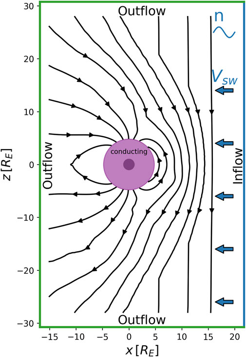
FIGURE 1. Schematic of the simulation setups.
With dipole moment D = −3110 nT (1/10th of the dipole strength of the real Earth) and
The tail is cutoff at − 15 RE to reduce the domain size while maintaining proper dayside structures. The spatial 2D configuration intrinsically disables the formation of the Dungey cycle of magnetic flux transport. We performed a series of test runs for different tail sizes on the nightside under coarser resolutions, and found no obvious impact on the dayside dynamics and wave propagations.
Initially, we imposed a southward upstream interplanetary magnetic field B = [0, 0, −5] nT. The majority of the simulation domain was filled with protons of density 2 amu/cc, velocity 600 km/s, and temperature 5 × 10⁵ K under the Maxwellian distribution. This lies in the fast solar wind regime above the 75% quantile in the proton temperature distribution from Wind spacecraft observation at one AU (Wilson et al., 2018), and is chosen for compensating the computationally-affordable velocity space resolution. We applied a half-cosine tapering of densities and velocities at t = 0 s for a smooth transition from radius r = 15 RE to the inner boundary at r≐5 RE with density 1 amu/cc and 0 velocity.
The inner boundary is treated as a perfectly conducting sphere, where the normal components of the magnetic fields and the electric fields in the halo cells are set to 0. A periodic boundary is applied for the out-of-plane y direction. The ± z boundaries and the downstream − x boundary were set to outflow conditions. As for the upstream + x boundary, we set a fixed Maxwellian condition for the first 400 s, with background parameters listed in Table 1. These parameters represent a fast solar wind with an Alfvén Mach number MA ∼ 8. While keeping realistic Alfvénic Mach numbers, we selected a relatively low average number density to make the spatial resolution closer to the ion inertial length, and a relatively high bulk velocity to speed up the runs.
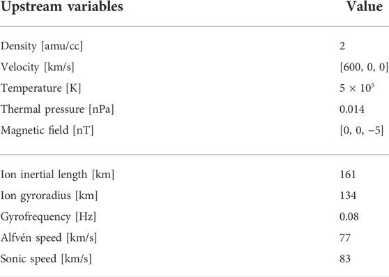
TABLE 1. Average upstream background states in the time-varying density run.
After t = 400 s, we switched on the time-varying conditions and introduced a sinusoidal density variation of period 150 s and amplitude 1 amu/cc (50% of the average) from the upstream boundary while keeping all other quantities fixed. The upstream halo cells were updated every 0.5 s. We ran the simulation for a total of 948 s. The output cadence was set to 0.5 s.
3 Results
3.1 Global view of dayside plasma moments and fields
Figure 2 shows filled contours of plasma density, in-plane bulk velocities, thermal pressure, magnetic field Bz and electric field Ey at t = 900 s, i.e. 500 s from the quasi-steady state. Supplementary Movie S1, 2 display the plasma moments, EM fields, plasma β, temperature anisotropy, and Mach numbers during the time-varying run. Across the shock, plasmas are heated preferably in the perpendicular direction. The median temperature anisotropy T⊥/T‖ (Movie 2(d)) is 2.3 in the magnetosheath, and it increases to
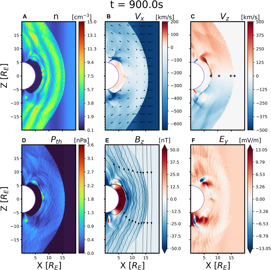
FIGURE 2. Selected plasma moments and EM field components from x ∈ [0, 20] RE, z ∈ [ − 20, 20] RE. All quantities are shown in linear scales. Continuous colormaps are applied to non-negative quantities, and divergent colormaps are applied to vector components, with zeros shown as white. Two separate linear color scales are used for positive and negative values of Vx. The arrows in the colorbars represent saturated colors with magnitudes that are equal or larger than the chosen values. Quivers of in-plane bulk velocity components are overplotted in (B), and in-plane magnetic field line projections are overplotted in (E). Four plus signs in (C) mark the virtual satellite locations in Figure 3.
When the imposed upstream density variations introduced by the time-varying boundary reach the magnetosheath, the plasma dynamics are modulated from the steady upstream condition case. The high-density stripes in the magnetosheath are caused by the upstream density pulse crests. At t = 900 s, three periods of 150 s Pc5 perturbations have already passed through the bow shock, and the fourth density crest is about to reach the shockfront. While the density fronts are straight along the z direction in the solar wind, they are deformed downstream of the bow shock because of the low speeds in the subsolar region. When a density stripe reaches the magnetopause, it mixes with the magnetic reconnection process triggered by southward IMF and gets dissipated near the magnetic diffusion region such that no clear single stripe structures can be identified.
Magnetic islands (2D flux rope structures) of different sizes are formed on the magnetopause, with high density and thermal pressure at the centers. These islands caused by dayside reconnection induce the transient fast magnetosonic bow waves in the magnetosheath, which are mostly visible in Figure 2A density, (b-c) bulk velocities, and (f) electric field Ey, and propagate towards higher latitudes along the magnetic field lines (Pfau-Kempf et al., 2016).
3.2 Virtual satellite analysis
Figure 3 shows time series collected by four representative virtual spacecrafts located in different regions along the Sun-Earth line, the locations of which are marked with black crosses in Figure 2C. The first satellite (a) is always located in the upstream solar wind. It takes

FIGURE 3. Virtual satellites tracking at four different locations along the subsolar line: (A) in the upstream solar wind, (B) across the bow shock, (C) in the middle of the magnetosheath, (D) inside the magnetosphere. Each satellite panel shows the plasma number density, velocity, dynamic ram pressure, thermal pressure, magnetic and electric field subsequently.
The second static satellite (b) crosses the bow shock twice during the run, first time around t = 590 s and second time around t = 700 s. This reflects the fact that the bow shock standoff distance shifts back and forth during this time interval, and later always stays in the +x direction relative to the satellite location. The imposed upstream density variation clearly modulates the locations of the bow shock: as density increases, the shock shifts earthward in space; as density decreases, the shock shifts further upstream. The shock crossing in (b) only happens during the second density pulse since the bow shock in general keeps expanding during our relatively short simulation time.
The third satellite (c) lies in the middle of the magnetosheath throughout the simulation. We observe two significant density crests at t = 695 and 860 s. These corresponds to the first and second density pulses from the upstream, travelling at plasma bulk speed. Two modes of oscillations, one with frequency
The fourth satellite (d) always stays within the magnetosphere, as shown by the positive Bz component. Three consecutive crests can be seen in the density time series line at around t = 570, 750, and 890 s. Since the stripe structure caused by the first density pulse has just reached the magnetopause around t = 900 s as shown in Figure 2, these perturbed crests inside the magnetosphere can only be directly driven by earthward propagating waves that travel faster than the bulk speed. The density and dominant magnetic field component Bz vary in-phase, indicating that this is a compressional mode. The perturbed EM field δBz and δEy are anti-correlated, meaning that this is an EM wave propagating along the x direction. These lead us to deduce that it is a fast magnetosonic mode, with Vx and Ey synchronizing in-phase, following the convective term in the generalized Ohm’s law Econv = −V ×B. We also see a periodic temporal transition of the flow direction from sunward (+x) to earthward (-x) at around t = 530 s, 680 s, and 830 s, respectively. The earthward flows last for about 70 s before switching back to sunward flows towards the magnetopause, which occurs during the decreasing density half of the upstream variation period. Perturbed signals inside the magnetosphere similar to Figure 3D can be detected all the way to the inner boundary. The fluctuations gets damped in all quantities except for the electric field as it penetrates further earthward.
The average local proton gyrofrequency Ωp is about 0.4 Hz at (c) in the magnetosheath and 1.0 Hz at (d) in the outer magnetosphere. Following the wave identification method suggested in Zhao et al. (2020), Figure 4 shows the wave oscillations between t = 500 and 900 s for virtual satellites (c) and (d). We perform band-pass 5th-order Butterworth filtering in two frequency bands, one between [0.02, 0.067] Hz (i.e. [15, 50] s) and the other between [0.1, 1.0] Hz (i.e [1, 10] s, limited by the Nyquist frequency). Both bands are below Ωp at the two virtual satellite locations. n, VA and B0 are the background moving box averaged density, Alfvén speed and magnetic field with window size 20 s. The two perpendicular directions

FIGURE 4. Filtered oscillations of normalized number density n, orthogonal perpendicular velocity components v⊥1, v⊥2, and parallel and perpendicular magnetic field B‖, B⊥1, B⊥2 at virtual satellite (C) in the magnetosheath and (D) in the magnetosphere.
3.3 Poynting flux analysis
For electromagnetic waves, wave vectors are parallel to the Poynting flux vectors. Given time series of electric field E and magnetic field B, the perturbation Poynting vector that represents the energy density flux of electromagnetic waves are defined as
where

FIGURE 5. Perturbation Poynting vectors parallel (first row) and perpendicular (second row) to the magnetic field in the simulation plane. The left and right four panels show band-pass filtered vector magnitudes between [0.1, 1.0] Hz and [0.02, 0.067] Hz respectively. The first and third columns show t = 670 s, and the second and forth columns show t = 750 s. The black quivers denote the direction of in-plane Poynting vectors, and the purple quivers denote the direction of in-plane ambient magnetic fields. Symmetric log scales with linear thresholds at 10–9 and 10–7 W/m2 are used for S‖ in the two bands, respectively. The arrows in the colorbars represent saturated colors with magnitudes that are equal or larger than the chosen values.
In the middle of the magnetosheath between [0.1, 1.0] Hz, we clearly identify waves that propagate mostly along the magnetic field lines away from low latitudes. However, there are still a small portion of EMIC waves traveling from high latitudes to low latitudes, as shown by S‖ at t = 670 s with red in z > 0 and blue in z < 0. The existence of S⊥ at the same time indicates that these waves do not propagate strictly along the magnetic field. This is further illustrated by the angles between
Between [0.02, 0.067] Hz, we see the dominant Poynting flux propagating at plasma bulk velocities, mostly perpendicular to the magnetic field lines as S⊥ is much larger than S‖ in the magnetosheath and

FIGURE 6. Sun-Earth line plots of plasma density, bulk velocity, dynamic ram pressure and thermal pressure, and EM fields from x = 7 to 17 RE, together with filled contours of Alfvén speed and plasma β in the dayside simulation domain. The annotations in the density line plot mark the first, second, and third density pulse peak, respectively. The vertical dashed red lines mark the location of the magnetopause defined by Bz = 0. The white dash lines show the extracted locations. The arrows in the colorbars represent saturated colors with magnitudes that are equal or larger than the chosen values.
The wave distributions are highly nonuniform in space. Supplementary Movie S3, 4 illustrate the dayside Poynting vectors for the high and low frequency band respectively. Overall both EMIC waves and mirror mode waves are more prominent when the magnetopause is located furthest from Earth (t = 670 s) and less prominent when the magnetopause is nearest to Earth (t = 750 s). However, this trend is not obvious from sample single virtual satellite observations as shown in Figure 4, partly due to the large spatial-temporal inhomogeneity. We will discuss this further in Section 3.4.2 and Section 4.
3.4 Subsolar line
3.4.1 Spatial analysis
For simplicity, we select all the cells along the central subsolar line and track plasma and field quantities along the line from the upstream solar wind (x = 17 RE) to the magnetosphere (x = 7 RE). Figure 6 shows the line plots with contours of Alfvén speed and plasma β on the dayside at t = 800 and 850 s. Under the purely southward IMF configuration, the magnetopause can be approximately defined as the location where Bz reverses sign. The magnetopause locations are denoted by the vertical red dashed lines. In the contour plots, they roughly overlap with the boundary where sharp gradients of Alfvén speed and plasma β occur. Discontinuities of various quantities also occur at the bow shock, located at x ∼ 15.5 RE. The density jump ratio across the bow shock ρd/ρu ∼ 3, same as the magnetic field tangential component jump ratio Bzu/Bzd, where subscripts “d” and “u” represent downstream and upstream respectively.
We identify three major features in the spatial effects of time-varying density perturbations on magnetospheric wave activity. Firstly, three density peaks are identified in the density panels, corresponding to crossings with small VA dark blue stripe regions in the Alfvén speed contours since VA ∝ ρ−1/2. These peaks travel at
Supplementary Movie S5 shows the subsolar line plots as a function of time. By tracking the locations where Vx and Ey change between positive and negative values during t = 600–670 s and 770–840 s, we find that the reversal points move at fast mode speeds. This further supports the deduction of fast wave propagation from the upstream in the virtual satellite analysis.
3.4.2 Space-time analysis
To incorporate the temporal changes into spatial analysis, we plotted 2D space-time filled contours along the Sun-Earth line in Figure 7. For each panel, the left side points towards the Earth and the right side points towards the upstream. The nose of the magnetopause as well as the bow shock crossing at each time are shown by the sharp discontinuities in various quantities. The magnetopause is constantly oscillating during the time-varying upstream density variations, with the subsolar point x coordinate shifting between 7.6 and 8.4 RE at an average velocity of

FIGURE 7. Space-time filled contours of density n, ram pressure Pram, electric field Ey, Alfvén Mach number MA, anisotropy, β‖, and parallel and perpendicular Poynting fluxes in two frequency bands along the subsolar line from x = 7 to 16.2 RE during t = 500–946s. The dashed lines in (A) represent the mean location of the discontinuities. The dotted lines in (D) represent wave tracking starting from multiple locations and times with local bulk velocities Vbulk in brown and additional local fast magnetosonic velocities Vfast in purple (parallel to Vbulk) and cyan (anti-parallel to Vbulk), respectively. A symmetric log scale with linear threshold at 10–9 W/m2 is applied for (E). The arrows in colorbars represent saturated colors with magnitudes outside the chosen ranges.
Multiple kinds of wave activities are shown in Figures 7A–D. To aid the identification of waves in the magnetosheath, we use a simple tracking technique to follow wave propagation on top of the MA filled contours. Starting from a given time and location, we calculated the local characteristic wave speeds to determine the destination in a fixed time step Δt = 2.5 s for the bulk velocity Vbulk and fast magnetosonic velocity Vfast tracking. The most obvious wave structure is shown by the large scale curly pattern of negative slopes in (a) density that closely follows Vbulk from the bow shock to the magnetopause. This suggests that these waves are static in the plasma frame. They have a period of around 20 s, and exist all over the magnetosheath under the temperature anisotropy T⊥/T‖ > 1.6 during the run. These are yet again features of the mirror mode waves.
The second kind of waves, shown by the traces Vbulk ± Vfast for the earthward propagating (+) and sunward propagating (-) branches, are the upstream density/pressure-driven fast magnetosonic modes. They can be observed most clearly from (b) Pram, (c) Ey, and (d) MA. The variation on the bow shock position associated with the periodic pulses generates the earthward propagating branch towards the magnetosphere, which is reflected at the magnetopause and travels back towards the bow shock. The transmitted density pulses encounter the reflected sunward propagating fast magnetosonic waves from the magnetopause and lead to enhancement of densities in the magnetosheath, shown by the quasi-periodic density perturbation along each streamline in Figure 7A. However, we do not observe secondary reflected waves at the bow shock propagating towards the magnetopause. Along the Sun-Earth line the magnetopause lags the bow shock motion by about 60 s, which approximately equals the fast wave travel time through the magnetosheath in the plasma rest frame. There is an one-to-one correspondence between the oscillating bow shock and magnetopause with time delay at the speed of Vfast for the simulated three periods. This clearly indicates that the disturbance of the magnetopause location is caused by fast modes launched from the interaction of the upstream variations with the bow shock. Figure 7B shows that Pram in the magnetosheath is mostly influenced by compressional fast waves, and in turn determines the pressure balance at the magnetopause.
The third type of waves in the magnetosheath appears as nearly horizontal bands in the contours and have relatively higher frequencies (about 0.16 Hz, or a period of 6 s), which are close to the local proton gyrofrequencies (
On the magnetospheric side of the magnetopause, two major patterns of oscillations are seen from alternating Ey. There is a large period (
Figures 7G,H show the perturbation Poynting flux components S‖ in the high frequency band and S⊥ in the low frequency band, the former corresponds to the EMIC modes while the latter corresponds to the mirror modes. The linear mirror instability criterion β⊥(T⊥/T‖ − 1) > 1 is fulfilled almost all the time in the magnetosheath. Lower power of S‖ at
3.5 Impact near the magnetopause
Figure 8 shows the bulk velocity Vx filled contours with in-plane velocity vectors and magnetic field lines in the low latitudes magnetosphere and magnetosheath region at three different times of the simulation. These frames represent the transition from the expansion phase on the left panel (t = 800 s) to the compression phase on the right panel (t = 850 s). Near the subsolar region, the boundary normals are nearly parallel to the x direction, therefore Vnormal ∼ Vx. Vnormal on both sides of the magnetopause may reverse sign due to the motion of the magnetopause. When the magnetopause is expanding at t = 800 s, the plasma velocity between z = ±3 RE points sunward on the order of 100 km/s on the magnetospheric side, and on the order of 10 km/s on the magnetosheath side. Contrarily, when the magnetopause is compressed via the fast mode signal as shown in Figure 7 at t = 850 s, earthward flows are observed with reversed order of magnitudes. In the magnetosheath, however, the sunward flows cannot penetrate deep towards the bow shock and stagnate within 2 RE away from the magnetopause, because the next period of fast waves has arrived due to the imposed upstream density variation. This dynamics leads to a periodic V-shape structure of bulk velocity along the Sun-Earth line that can be inferred from Figure 7B on the magnetosheath side near the magnetopause since

FIGURE 8. Filled contours of bulk velocity Vx, with in-plane velocity quivers in black and magnetic field lines in olive. The red dotted lines denote the magnetopause where Bz = 0. The violet crosses and dots denote computed X-points and O-points from the magnetic flux function, respectively. The three snapshots at t = 800s, 825s, and 850s represent the transition from expansion phase to compression phase of the magnetopause.
The periodic change in velocity does not lead to a clear trend in the magnetic reconnection rate. We identified the X-points and O-points for each frame based on the saddle points and local extrema calculated from the magnetic flux function as done in Hoilijoki et al. (2017), which are shown by the violet crosses and dots in Figure 8. At t = 800 s, the X-point near z = -1 RE is located right next to a magnetic island, and the local flow on the magnetosheath side points earthward, despite the overall expansion of the magnetopause. 25 s later at t = 825 s, the expansion stops. Velocities near the central magnetopause are small on both sides and X-points shift to higher latitudes instead of disappearing. After another 25 s at t = 850 s, the flow is mostly earthward, and X-points can be again identified at lower latitudes. We estimated the dimensionless local reconnection rate at each X-point with the electric field Ey at the X-point normalized by the inflow Alfvén speed and magnetic field strength. Although the rates are on the order of 0.1, the exact values are very sensitive to (1) the identified X-point location, (2) the inflow upstream value extraction location, and (3) the definition of normal direction to the X-line configuration. Hoilijoki et al. (2017) reported a statistical survey on the dayside reconnection rate from a steady upstream 2D Vlasiator run, where significant variations may be found for individual X-point reconnection. Figure 2 in Hoilijoki et al. (2017) also showed that even for steady upstream conditions the X-lines may shift between ±3 RE along the z direction. Here we observe a trend of fewer low latitude X-points during flow reversal times, and find no evidence of altering reconnection rates by the influence of upstream density/pressure variation and the following magnetopause motion under the current simulated global magnetosphere settings.
4 Discussion
In the dayside magnetosheath, positively correlated δn and δB‖ in the [0.1, 1.0] Hz band has been reported by Lacombe et al. (1992) from ISEE1-2 and Zhao et al. (2019) from MMS observations. Lacombe et al. (1992) suggested that the correlation might be explained by the nearly parallel helium cut-off mode with a frequency that is very close to an unstable EMIC mode. However, this is not possible in our simulation since we only include hydrogen ion. The weak compressional mode we see in the simulated magnetosheath is more likely a fast mode originated from reconnection or the motion of the magnetopause, as suggested in Supplementary Movie S3.
Responses of the magnetosphere to an impulse or harmonic excitation motivated many studies in the past. The monochromatic density variations studied in our simulation can be comparable to the impact of tangential discontinuities (TDs) with a perpendicular shock. This was discussed by Wu et al. (1993) under the 1D ideal MHD approximation. They studied two cases with both theoretical predictions and MHD simulations: the first case considered a sharp density jump ratio two and the second considered a sharp density jump ratio 0.5, while keeping all other quantities continuous. They predicted that a density jump excites a fast shock propagating downstream, whereas a density drop should trigger a fast rarefaction wave, again propagating downstream. Both of these have been detected from our hybrid simulation. A similar process has been reported from ideal MHD results in Park et al. (2002) with a single upstream density pulse. Since the density pulse we impose in this study is more continuous than discrete, we constantly observe downstream propagating fast modes, alternating between fast shocks and rarefaction waves in different phases (e.g. Figure 7D). Samsonov et al. (2006) found from a local 3D ideal MHD model that the time of propagation of the forward fast shock through the subsolar magnetosheath is about 1 minute, which is similar to the transit time found from our simulation. Despite the qualitative agreement, we note that, unlike in the 1D ideal MHD theory, the state on one side of a discontinuity beyond an anisotropic MHD model cannot be fully determined in terms of quantities on the other side using the Rankine-Hugoniot (RH) relations (Hudson, 1970).
Maynard et al. (2007) studied a TD observed by the Advanced Composition Explorer satellite (ACE) and the Polar satellite with an 145° rotation of the IMF and more than a factor of 2 decrease in the upstream density. The interaction between the TD and the bow shock triggered a fast rarefaction wave propagating towards the magnetopause surrounded by slow mode transitions, as shown by the Polar satellite data in the magnetosheath in their Figure 3. The 3D resistive MHD simulation demonstrated a downstream propagating fast mode rarefaction wave and suggested a corresponding reflected fast wave propagated back towards the bow shock when the magnetopause began to expand, the latter of which cannot occur in the Wu et al. (1993) model because of the open downstream boundary. Both the forward and backward propagating fast modes are observed in our simulation results. However, unlike the isotropic MHD models, in our hybrid model the magnetosheath is dominated by mirror modes on the large scale. Therefore the correlations between density and magnetic field are mostly negative in the magnetosheath at low frequency ranges, which makes direct fast mode signals from the harmonic upstream variation hardly detectable. If instead we introduced a strong isolated impulse in the solar wind (e.g., Archer et al. (2021)), we would expect a similar positive correlated density and magnetic field fast mode region surrounded by negative correlated slow/mirror mode regions.
Using 2 years of Cluster magnetometer data, Soucek et al. (2015) reported more common mirror mode wave occurrences in the magnetosheath under quasi-perpendicular bow shocks with higher MA (between 4–16), while EMIC modes were only observed when MA < 8. In this study, we use the perturbation Poynting flux as an indicator for wave occurrences and present a noon-midnight meridional plane global picture of wave activities. However, one should be cautious in comparing our simulation results to the Cluster survey. Firstly, the average background conditions in our simulation is different from Cluster observations. For instance, compared with Soucek et al. (2015) Figure 3, we have higher temperature anisotropy in the magnetosheath especially near the magnetopause (Figure 7E; Supplementary Movie 2D, which leads to the fulfillment of mirror mode linear instability criterion almost all the time. Secondly, the event selection criteria for EMIC waves
Density/pressure variations from the solar wind were also shown to be capable of causing field line resonances (FLRs, Tamao, (1964)) from 3D global MHD simulations, e.g. Claudepierre et al. (2009, 2010, 2016); Hartinger et al. (2014), and modulating field-aligned currents (FACs) in the magnetosphere-ionosphere (MI) coupled system (Motoba et al., 2007). Unfortunately FLRs are not included in our simulation. A necessary condition for FLR to occur is a finite, nonzero azimuthal wavenumber (kϕ in cylindrical coordinates, or ky in Cartesian coordinates). Since the y axis is periodic with no prescribed oscillations in our 2D meridional plane configuration, ky is essentially 0. A proper description of FACs also requires 3D spatial geometry, as well as an ionosphere model and a plasmasphere model at the inner boundary, which is currently under development (Ganse et al. (2022) in prep.).
Kepko et al. (2020) and the references thereafter reported that strongest solar wind density variations are usually observed in the slow solar wind (Vsw < 550 km/s), and the frequencies associated with the density variation typically lie within [0.5, 4] mHz. Recently, Di Matteo et al. (2022) presented a comprehensive case study during the interaction of the magnetosphere with two interplanetary shocks that were followed by a train of 90 min solar wind periodic density structures (PDS) with bulk velocity around 400 km/s. They identified directly triggered geosynchronous orbit magnetic field perturbations from PDS of frequencies roughly below 3 mHz and largely triggered modes in higher frequency ranges. The simulated solar wind conditions in this study has 6.7 mHz upstream density variations within the fast solar wind velocity range, both of which are larger the reported commonly observed values. This is a compromise between simulating periodic fluctuations in the relevant period range for magnetospheric waves (i.e. Pc5) and the affordable computational cost at decent resolutions. The PDS event presented in Di Matteo et al. (2022) corresponds to MA roughly between [5.3, 9.4], which is comparable to the range [5.7, 9.8] in the current simulation. Under more typical PDS solar wind conditions, we expect similar fast wave generation and propagation processes downstream of the bow shock, and similar trends in modulations to the high frequency EMIC and mirror waves spatial-temporal occurrence. However, cautions must be taken when discussing the specific discrete frequencies that are related to eigenmodes of FLR. The locations and frequencies of FLR depends on both the internal and external plasma and field quantities. Since in our current 2D setup FLR cannot be triggered, this complicated scenario is somehow circumvented. Nevertheless, it should be carefully considered in the following study under 3D space configuration.
Besides the run that is thoroughly investigated in this paper, we also performed 2D equatorial plane simulations for comparison. A quasi-perpendicular shock in the X-Y plane requires solar wind magnetic field in the Y-Z plane. When the upstream magnetic field lies purely along the out-of-plane z direction, a huge temperature anisotropy (T⊥/T‖ > 20) is generated downstream of the bow shock due to the lack of parallel heating, which is different from the 2D meridional or 3D cases. This happens when the model goes beyond isotropic MHD, where pressure is described by at least the parallel and perpendicular components. When the upstream magnetic field lies purely along the y direction, we can obtain wave modes similar to the X-Z meridional plane case. However, the run suffers from the ambiguity of magnetopause definition and a lack of magnetic flux transfer mechanism; thus it is hard to distinguish magnetosphere from magnetosheath, and the magnetic flux pile-up leads to drastic expansion of the bow shock as time evolves. Although finite ky is allowed in the azimuthal direction, there is still no FLR because of the missing of toroidal Alfvén modes propagating along the out-of-plane ambient field lines.
5 Conclusion
In this study, we applied a 2D hybrid-Vlasov model to study the influence of upstream density variations in the Earth dayside magnetosphere and magnetosheath. The periodic density pulses generate fast magnetosonic modes propagating downstream of the quasi-perpendicular bow shock and reflected fast modes at the magnetopause, both of which mix with the mirror mode and EMIC mode triggered by temperature anisotropy in the magnetosheath. The simulation provides a global view of the interaction of the upstream density variations with near-Earth space, showing that they form alternating stripes of enhanced and decreased density in the magnetosheath that remain for an extended period in the downstream because of the relatively slow flow in the subsolar region. This is likely representative of what happens in the actual magnetosheath because solar wind density variations generally have transverse scales much larger than the size of Earth’s dayside magnetosphere (Richardson and Paularena, 2001; Matsui et al., 2002), although recent study by Burkholder et al. (2020) has also showed the potential importance introduced by upstream spatial gradients. There are two steps in the interaction of density changes with the magnetosheath: first when fast modes are launched from the bow shock, and second as the density stripes propagate through the magnetosheath together with the plasma. Despite the spatial-temporal inhomogeneity of waves, less prominent EMIC and mirror mode wave activities near the center of magnetosheath are observed with decreasing upstream Mach number. The EMIC wave occurrence is strongly related to pressure anisotropy and β‖, both vary as a function of the upstream conditions, whereas the mirror mode occurrence is highly influenced by fast rarefaction waves generated from upstream density variations.
In the future, we anticipate longer runs, preferably in 3D that couple with an ionosphere model, to investigate the wave propagation and current responses further inside the magnetosphere in the ULF regime.
Data availability statement
Vlasiator is distributed under the GPL-2 open-source licence. The Julia package Vlasiator.jl is used for 550 data post-processing. The run described here contains restart files of 1.1 TB each and 0.5 TB of output files during time-varying inputs, which are kept in storage at the University of Helsinki. Data presented in this paper can be accessed by following the data policy on the Vlasiator website https://github.com/fmihpc/vlasiator.
Author contributions
HZ developed the time-varying boundary condition modules for Vlasiator, ran the simulation and performed the data analysis. LT is the principal investigator (PI) of the RESSAC project and helped with the data analysis and interpretation of the results. YP-K and MB participated in debugging and monitoring the simulation outputs. VT, MD, JH, MG, IZ, GC, MA, HG, ML, KP, KH, FT, UG, and EG contributed to the data analysis and discussions. MP is the PI of the Vlasiator model. All co-authors participated in the discussion and verification of the results as well as contributed to the drafts.
Funding
This project was carried out with the support from the University of Helsinki (3-year research grant 2020-2022) and the Academy of Finland (grant numbers. 322544 and 328893). The work leading to these results has been carried out in the Finnish Centre of Excellence in Research of Sustainable Space (Academy of Finland grant number 312351). Pfau-Kempf is supported by Academy of Finland 339756, and Grandin is supported by Academy of Finland 338629. We acknowledge the European Research Council for Starting grant 200141-QuESpace, with which Vlasiator was developed, and Consolidator grant 682068-PRESTISSIMO awarded to further develop Vlasiator and use it for scientific investigations.
Acknowledgments
The authors thank Dr. Yuxi Chen for some insightful discussions about global 2D simulations, Dr. Sanni Hoilijoki for the discussions on mirror modes, Dr. Jinsong Zhao for the discussions on wave identifications. The CSC-IT Center for Science in Finland is acknowledged for providing computing time leading to the results shown here. We thank the Finnish Grid and Cloud Infrastructure (FGCI) and specifically Juha Antero Helin from the University of Helsinki computing services for supporting this project with computational and data storage resources.
Conflict of interest
The authors declare that the research was conducted in the absence of any commercial or financial relationships that could be construed as a potential conflict of interest.
Publisher’s note
All claims expressed in this article are solely those of the authors and do not necessarily represent those of their affiliated organizations, or those of the publisher, the editors and the reviewers. Any product that may be evaluated in this article, or claim that may be made by its manufacturer, is not guaranteed or endorsed by the publisher.
Supplementary material
The Supplementary Material for this article can be found online at: https://www.frontiersin.org/articles/10.3389/fspas.2022.984918/full#supplementary-material
References
Archer, M., Hartinger, M., Plaschke, F., Southwood, D., and Rastaetter, L. (2021). Magnetopause ripples going against the flow form azimuthally stationary surface waves. Nat. Commun. 12, 1–14. doi:10.1038/s41467-021-25923-7
Archer, M. O., Southwood, D. J., Hartinger, M., Rastaetter, L., and Wright, A. (2022). How a realistic magnetosphere alters the polarizations of surface, fast magnetosonic, and alfvén waves. J. Geophys. Res. Space Phys. 127, e2021JA030032. doi:10.1029/2021JA030032
Archer, M., Turner, D., Eastwood, J., Horbury, T., and Schwartz, S. (2014). The role of pressure gradients in driving sunward magnetosheath flows and magnetopause motion. J. Geophys. Res. Space Phys. 119, 8117–8125. doi:10.1002/2014JA020342
Baddeley, L. J., Lorentzen, D. A., Partamies, N., Denig, M., Pilipenko, V., Oksavik, K., et al. (2017). Equatorward propagating auroral arcs driven by ulf wave activity: Multipoint ground-and space-based observations in the dusk sector auroral oval. J. Geophys. Res. Space Phys. 122, 5591–5605. doi:10.1002/2016ja023427
Burkholder, B., Nykyri, K., and Ma, X. (2020). Use of the l1 constellation as a multispacecraft solar wind monitor. JGR. Space Phys. 125, e2020JA027978. doi:10.1029/2020JA027978
Claudepierre, S., Hudson, M., Lotko, W., Lyon, J., and Denton, R. (2010). Solar wind driving of magnetospheric ulf waves: Field line resonances driven by dynamic pressure fluctuations. J. Geophys. Res. 115. doi:10.1029/2010JA015399
Claudepierre, S., Toffoletto, F., and Wiltberger, M. (2016). Global mhd modeling of resonant ulf waves: Simulations with and without a plasmasphere. JGR. Space Phys. 121, 227–244. doi:10.1002/2015ja022048
Claudepierre, S., Wiltberger, M., Elkington, S., Lotko, W., and Hudson, M. (2009). Magnetospheric cavity modes driven by solar wind dynamic pressure fluctuations. Geophys. Res. Lett. 36, L13101. doi:10.1029/2009GL039045
Daldorff, L. K., Tóth, G., Gombosi, T. I., Lapenta, G., Amaya, J., Markidis, S., et al. (2014). Two-way coupling of a global hall magnetohydrodynamics model with a local implicit particle-in-cell model. J. Comput. Phys. 268, 236–254. doi:10.1016/j.jcp.2014.03.009
Di Matteo, S., Villante, U., Viall, N., Kepko, L., and Wallace, S. (2022). On differentiating multiple types of ulf magnetospheric waves in response to solar wind periodic density structures. J. Geophys. Res. Space Phys. 127, e2021JA030144. doi:10.1029/2021JA030144
Dubart, M., Ganse, U., Osmane, A., Johlander, A., Battarbee, M., Grandin, M., et al. (2020). Resolution dependence of magnetosheath waves in global hybrid-vlasov simulations. Ann. Geophys. 38, 1283–1298. doi:10.5194/angeo-38-1283-2020
Elkington, S. R. (2006). A review of ulf interactions with radiation belt electrons. Magnetos. ULF waves Synthesis new Dir. 169, 177–193. doi:10.1029/169GM12
Hartinger, M., Moldwin, M. B., Zou, S., Bonnell, J. W., and Angelopoulos, V. (2015). Ulf wave electromagnetic energy flux into the ionosphere: Joule heating implications. J. Geophys. Res. Space Phys. 120, 494–510. doi:10.1002/2014JA020129
Hartinger, M., Welling, D., Viall, N. M., Moldwin, M. B., and Ridley, A. (2014). The effect of magnetopause motion on fast mode resonance. J. Geophys. Res. Space Phys. 119, 8212–8227. doi:10.1002/2014JA020401
Heyns, M., Lotz, S., and Gaunt, C. (2021). Geomagnetic pulsations driving geomagnetically induced currents. Space weather. 19, e2020SW002557. doi:10.1029/2020sw002557
Hoilijoki, S., Ganse, U., Pfau-Kempf, Y., Cassak, P. A., Walsh, B. M., Hietala, H., et al. (2017). Reconnection rates and x line motion at the magnetopause: Global 2d-3v hybrid-vlasov simulation results. JGR. Space Phys. 122, 2877–2888. doi:10.1002/2016JA023709
Hoilijoki, S., Palmroth, M., Walsh, B. M., Pfau-Kempf, Y., von Alfthan, S., Ganse, U., et al. (2016). Global MHD modeling of resonant ULF waves: Simulations with and without a plasmasphere. JGR. Space Phys. 121, 227–244. doi:10.1002/2015JA022048
Hudson, P. (1970). Discontinuities in an anisotropic plasma and their identification in the solar wind. Planet. Space Sci. 18, 1611–1622. doi:10.1016/0032-0633(70)90036-X
Jacobs, J., Kato, Y., Matsushita, S., and Troitskaya, V. (1964). Classification of geomagnetic micropulsations. J. Geophys. Res. 69, 180–181. doi:10.1029/JZ069i001p00180
Johnson, J. R., and Cheng, C. (1997). Global structure of mirror modes in the magnetosheath. J. Geophys. Res. 102, 7179–7189. doi:10.1029/96JA03949
Kepko, L., Spence, H. E., and Singer, H. (2002). Ulf waves in the solar wind as direct drivers of magnetospheric pulsations. Geophys. Res. Lett. 29, 391–394. doi:10.1029/2001GL014405
Kepko, L., Viall, N. M., and Wolfinger, K. (2020). Inherent length scales of periodic mesoscale density structures in the solar wind over two solar cycles. JGR. Space Phys. 125, e2020JA028037. doi:10.1029/2020JA028037
Kepko, L., and Viall, N. (2019). The source, significance, and magnetospheric impact of periodic density structures within stream interaction regions. JGR. Space Phys. 124, 7722–7743. doi:10.1029/2019JA026962
Kessel, R. L. (2008). Solar wind excitation of pc5 fluctuations in the magnetosphere and on the ground. J. Geophys. Res. 113. doi:10.1029/2007JA012255
Kozyreva, O. V., Pilipenko, V. A., Bland, E. C., Baddeley, L. J., and Zakharov, V. I. (2020). Periodic modulation of the upper ionosphere by ulf waves as observed simultaneously by superdarn radars and gps/tec technique. J. Geophys. Res. Space Phys. 125, e2020JA028032. doi:10.1029/2020ja028032
Lacombe, C., Pantellini, F., Hubert, D., Harvey, C., Mangeney, A., Belmont, G., et al. (1992). Mirror and alfvenic waves observed by isee 1-2 during crossings of the earth’s bow shock. Ann. Geophys. 10, 772–784.
Matsui, H., Farrugia, C. J., and Torbert, R. B. (2002). Wind-ace solar wind correlations, 1999: An approach through spectral analysis. J. Geophys. Res. 107, 1355–SSH7. doi:10.1029/2002JA009251
Maynard, N., Burke, W., Ober, D., Farrugia, C. J., Kucharek, H., Lester, M., et al. (2007). Interaction of the bow shock with a tangential discontinuity and solar wind density decrease: Observations of predicted fast mode waves and magnetosheath merging. J. Geophys. Res. 112. doi:10.1029/2007JA012293
Motoba, T., Fujita, S., Kikuchi, T., and Tanaka, T. (2007). Solar wind dynamic pressure forced oscillation of the magnetosphere-ionosphere coupling system: A numerical simulation of directly pressure-forced geomagnetic pulsations. J. Geophys. Res. 112. doi:10.1029/2006JA012193
Palmroth, M., Archer, M., Vainio, R., Hietala, H., Pfau-Kempf, Y., Hoilijoki, S., et al. (2015). Ulf foreshock under radial imf: Themis observations and global kinetic simulation vlasiator results compared. J. Geophys. Res. Space Phys. 120, 8782–8798. doi:10.1002/2015JA021526
Palmroth, M., Ganse, U., Pfau-Kempf, Y., Battarbee, M., Turc, L., Brito, T., et al. (2018). Vlasov methods in space physics and astrophysics. Living Rev. comput. Astrophys. 4, 1–54. doi:10.1007/s41115-018-0003-2
Palmroth, M., Raptis, S., Suni, J., Karlsson, T., Turc, L., Johlander, A., et al. (2021). Magnetosheath jet evolution as a function of lifetime: Global hybrid-vlasov simulations compared to mms observations. Ann. Geophys. 39, 289–308. doi:10.5194/angeo-39-289-2021
Park, S., Lee, D.-Y., Min, K., and Seon, J. (2002). Three-dimensional magnetohydrodynamic simulations on the interaction of interplanetary density pulses with the bow shock. Phys. Plasmas 9, 1764–1774. doi:10.1063/1.1461847
Pfau-Kempf, Y., Battarbee, M., Ganse, U., Hoilijoki, S., Turc, L., von Alfthan, S., et al. (2018). On the importance of spatial and velocity resolution in the hybrid-vlasov modeling of collisionless shocks. Front. Phys. 6, 44. doi:10.3389/fphy.2018.00044
Pfau-Kempf, Y., Hietala, H., Milan, S. E., Juusola, L., Hoilijoki, S., Ganse, U., et al. (2016). Evidence for transient, local ion foreshocks caused by dayside magnetopause reconnection. Ann. Geophys. 34, 943–959. doi:10.5194/angeo-34-943-2016
Plaschke, F., Glassmeier, K.-H., Auster, H., Angelopoulos, V., Constantinescu, O., Fornaçon, K.-H., et al. (2009). Statistical study of the magnetopause motion: First results from themis. J. Geophys. Res. 114. doi:10.1029/2008JA013423
Richardson, J. D., and Paularena, K. I. (2001). Plasma and magnetic field correlations in the solar wind. J. Geophys. Res. 106, 239–251. doi:10.1029/2000JA000071
Ripoll, J.-F., Claudepierre, S., Ukhorskiy, A., Colpitts, C., Li, X., Fennell, J., et al. (2020). Particle dynamics in the earth’s radiation belts: Review of current research and open questions. J. Geophys. Res. Space Phys. 125, e2019JA026735. doi:10.1029/2019JA026735
Samsonov, A., Němeček, Z., and Šafránková, J. (2006). Numerical mhd modeling of propagation of interplanetary shock through the magnetosheath. J. Geophys. Res. 111, A08210. doi:10.1029/2005JA011537
Schwartz, S., Burgess, D., and Moses, J. (1996). Low-frequency waves in the earth’s magnetosheath: Present status. Ann. Geophys. 14, 1134–1150. doi:10.1007/s00585-996-1134-z
Soucek, J., Escoubet, C. P., and Grison, B. (2015). Magnetosheath plasma stability and ulf wave occurrence as a function of location in the magnetosheath and upstream bow shock parameters. J. Geophys. Res. Space Phys. 120, 2838–2850. doi:10.1002/2015JA021087
Soucek, J., Lucek, E., and Dandouras, I. (2008). Properties of magnetosheath mirror modes observed by cluster and their response to changes in plasma parameters. J. Geophys. Res. 113. doi:10.1029/2007JA012649
Southwood, D. J., and Kivelson, M. G. (1993). Mirror instability: 1. Physical mechanism of linear instability. J. Geophys. Res. 98, 9181–9187. doi:10.1029/92JA02837
Takahashi, K., Turc, L., Kilpua, E., Takahashi, N., Dimmock, A., Kajdic, P., et al. (2021). Propagation of ultralow-frequency waves from the ion foreshock into the magnetosphere during the passage of a magnetic cloud. J. Geophys. Res. Space Phys. 126, e2020JA028474. doi:10.1029/2020JA028474
Tamao, T. (1964). The structure of three-dimensional hydromagnetic waves in a uniform cold plasma. J. Geomagn. Geoelec. 16, 89–114. doi:10.5636/jgg.16.89
Turc, L., Ganse, U., Pfau-Kempf, Y., Hoilijoki, S., Battarbee, M., Juusola, L., et al. (2018). Foreshock properties at typical and enhanced interplanetary magnetic field strengths: Results from hybrid-vlasov simulations. J. Geophys. Res. Space Phys. 123, 5476–5493. doi:10.1029/2018JA025466
Viall, N., Kepko, L., and Spence, H. E. (2009). Relative occurrence rates and connection of discrete frequency oscillations in the solar wind density and dayside magnetosphere. J. Geophys. Res. 114. doi:10.1029/2008JA013334
Von Alfthan, S., Pokhotelov, D., Kempf, Y., Hoilijoki, S., Honkonen, I., Sandroos, A., et al. (2014). Vlasiator: First global hybrid-vlasov simulations of earth’s foreshock and magnetosheath. J. Atmos. Solar-Terrestrial Phys. 120, 24–35. doi:10.1016/j.jastp.2014.08.012
Wang, B., Nishimura, Y., Hartinger, M., Sivadas, N., Lyons, L. L., Varney, R. H., et al. (2020). Ionospheric modulation by storm time pc5 ulf pulsations and the structure detected by pfisr-themis conjunction. Geophys. Res. Lett. 47, e2020GL089060. doi:10.1029/2020GL089060
Wilson, L. B., Stevens, M. L., Kasper, J. C., Klein, K. G., Maruca, B. A., Bale, S. D., et al. (2018). The statistical properties of solar wind temperature parameters near 1 au. Astrophys. J. Suppl. Ser. 236, 41. doi:10.3847/1538-4365/aab71c
Wu, B.-H., Mandt, M., Lee, L., and Chao, J. (1993). Magnetospheric response to solar wind dynamic pressure variations: Interaction of interplanetary tangential discontinuities with the bow shock. J. Geophys. Res. 98, 21297–21311. doi:10.1029/93JA01013
Zerroukat, M., and Allen, T. (2012). A three-dimensional monotone and conservative semi-Lagrangian scheme (slice-3d) for transport problems. Q. J. R. Meteorol. Soc. 138, 1640–1651. doi:10.1002/qj.1902
Zhao, J., Wang, T., Dunlop, M., Shi, C., He, J., Dong, X., et al. (2019). Large-amplitude electromagnetic ion cyclotron waves and density fluctuations in the flank of the earth’s magnetosheath. Geophys. Res. Lett. 46, 4545–4553. doi:10.1029/2019GL081964
Zhao, J., Wang, T., Graham, D. B., He, J., Liu, W., Dunlop, M. W., et al. (2020). Identification of the nature of electromagnetic waves near the proton-cyclotron frequency in solar-terrestrial plasmas. Astrophys. J. 890, 17. doi:10.3847/1538-4357/ab672f
Keywords: space physics, plasma, magnetosheath, solar wind, simulation, kinetic, hybrid, magnetosphere
Citation: Zhou H, Turc L, Pfau-Kempf Y, Battarbee M, Tarvus V, Dubart M, George H, Cozzani G, Grandin M, Ganse U, Alho M, Johlander A, Suni J, Bussov M, Papadakis K, Horaites K, Zaitsev I, Tesema F, Gordeev E and Palmroth M (2022) Magnetospheric responses to solar wind Pc5 density fluctuations: Results from 2D hybrid Vlasov simulation. Front. Astron. Space Sci. 9:984918. doi: 10.3389/fspas.2022.984918
Received: 02 July 2022; Accepted: 01 August 2022;
Published: 02 September 2022.
Edited by:
David Ruffolo, Mahidol University, ThailandReviewed by:
Amar Kakad, Indian Institute of Geomagnetism (IIG), IndiaSimone Di Matteo, The Catholic University of America, United States
Copyright © 2022 Zhou, Turc, Pfau-Kempf, Battarbee, Tarvus, Dubart, George, Cozzani, Grandin, Ganse, Alho, Johlander, Suni, Bussov, Papadakis, Horaites, Zaitsev, Tesema, Gordeev and Palmroth . This is an open-access article distributed under the terms of the Creative Commons Attribution License (CC BY). The use, distribution or reproduction in other forums is permitted, provided the original author(s) and the copyright owner(s) are credited and that the original publication in this journal is cited, in accordance with accepted academic practice. No use, distribution or reproduction is permitted which does not comply with these terms.
*Correspondence: Hongyang Zhou, aG9uZ3lhbmcuemhvdUBoZWxzaW5raS5maQ==