 Joseph E. Borovsky
95% of researchers rate our articles as excellent or good
Learn more about the work of our research integrity team to safeguard the quality of each article we publish.
Find out more
ORIGINAL RESEARCH article
Front. Astron. Space Sci. , 05 January 2023
Sec. Space Physics
Volume 9 - 2022 | https://doi.org/10.3389/fspas.2022.975135
This article is part of the Research Topic Solar Wind - Magnetosphere Interaction View all 18 articles
There is a general consensus that fluctuations in the solar wind magnetic field and/or the Alfvenicity of the solar wind drive a solar wind-magnetosphere interaction. 11 years of hourly-averaged solar wind and magnetospheric geomagnetic indices are used to further examine this hypothesis in detail, confirming that geomagnetic activity statistically increases with the amplitude of upstream fluctuations and with the Alfvénicity, even when solar-wind reconnection driver functions are weak and reconnection on the dayside magnetopause should vanish. A comparison finds that the fluctuation-amplitude effect appears to be stronger than the Alfvénicity effect. In contradiction to the generally accepted hypothesis of driving an interaction, it is also demonstrated that many solar wind parameters are correlated with the fluctuation amplitude and the Alfvénicity. As a result, we caution against immediately concluding that the latter two parameters physically drive the overall solar-wind/magnetosphere interaction: the fluctuation amplitude and Alfvénicity could be acting as proxies for other more-relevant variables. More decisive studies are needed, perhaps focusing on the roles of ubiquitous solar-wind strong current sheets and velocity shears, which drive the measured amplitudes and Alfvénicities of the upstream solar-wind fluctuations.
The impact of upstream solar-wind fluctuations on the driving of the Earth’s magnetosphere has been of interest for decades [cf. the recent review by D’Amicis et al., (2020)]. Early interest was on the association between low-frequency Alfvénic magnetic-field fluctuations in high-speed-stream solar wind with high-speed-stream-driven geomagnetic activity, so-called “HILDCAA” events (Tsurutani and Gonzalez, 1987; Tsurutani et al., 1995; Tsurutani et al., 1999; Gonzalez et al., 1999; Diego et al., 2005). During the high-speed streams coordinated few-hour periodicities are seen in the properties of the solar-wind fluctuations and in the behavior of geomagnetic indices (e.g., Tsurutani and Gonzalez, 1987; Diego et al., 2005). For these high-speed-stream driving events the underlying physical mechanism driving the Earth was hypothesized to be enhanced dayside reconnection during the southward–IMF portions of the low-frequency magnetic fluctuations (Gonzalez et al., 1999; Tsurutani et al., 1999). This hypothesis is consistent with the observed Russell-McPherron-effect variation of magnetospheric activity during high-speed stream driving (Borovsky and Steinberg, 2006a; McPherron et al., 2009). Voros et al., (2002) proposed a further hypothesis that the fluctuating direction of the solar-wind magnetic field gives rise to patchy reconnection on the dayside magnetosphere.
Jankovicova et al., (2008a), Jankovicova et al., (2008b) focused their solar-wind/magnetosphere data-analysis research on the correlations between geomagnetic activity and 1) the solar-wind fluctuation kurtosis and 2) the solar wind “Shebalin angle” θ. The Shebalin angle is directly related to the normalized fluctuation amplitude ΔB/B of the solar wind fluctuations, where ΔB is the vector fluctuation amplitude of the magnetic-field vector
Beyond reconnection driving of the magnetosphere, evidence has been found of an enhanced driving associated with the amplitude of solar-wind upstream magnetic-field fluctuations (Borovsky and Funsten, 2003; Borovsky and Steinberg, 2006b; Borovsky, 2006; Borovsky, 2013), even during intervals of strongly northward IMF when dayside reconnection should not be occurring (Borovsky and Funsten, 2003; Borovsky and Steinberg, 2006b; Osmane et al., 2015). The increase in the amplitude of the solar-wind fluctuations was correlated with about a 100-nT increase in the AE index. In analogy with the “freestream turbulence effect” in wind tunnels (Kwok and Melborne, 1980; Sullerey and Sayeed Khan, 1983; Blair, 1983a; Blair, 1983b; Hoffmann, 1991; Hoffmann and Mohammadi, 1991; Wu and Faeth, 1994; Volino, 1998; Pal, 1985; Thole and Bogard, 1996; Volino et al., 2003), Borovsky and Funsten (2003) hypothesized that the beyond-reconnection driving mechanism was an enhanced eddy viscosity in the solar wind plasma associated with the enhanced fluctuations [see Figure 1 of Borovsky (2006)]: the enhanced eddy viscosity would more-efficiently transfer momentum from the solar wind to the magnetosphere. A specific freestream-turbulence driver function was derived for the supersonic solar wind (cf. Section 2).
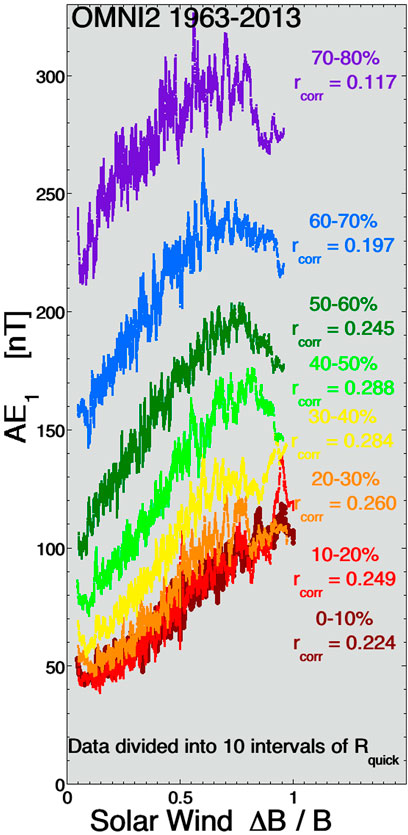
FIGURE 1. For times when the value of Rquick is in 10-percent intervals, 300-point running averages of the one-hour-lagged AE index is plotted as a function of the amplitude ΔB/B of the upstream solar-wind turbulence.
D’Amicis et al., (2007), D’Amicis et al., (2009), D’Amicis et al., (2010) focused their solar-wind/magnetosphere data analysis on the driving of the Earth’s magnetosphere by highly Alfvénic fluctuations during high-speed streams, finding clear evidence of the relationship between Alfvénic fluctuations in the solar wind and elevated values of the AE index activity.
Osmane et al., (2015) examined the relation between the occurrence distributions of AL-index values as functions of the mean spectral power of solar-wind Bz fluctuations for both average southward and average northward IMF. That study found effects of the magnetic-field fluctuations impacting the AL index at levels up to 200 nT.
An important question is whether this enhanced (beyond reconnection) driving of the Earth’s magnetosphere correlated with solar-wind fluctuations is real in the sense that the solar-wind fluctuations are physically doing something to the Earth’s magnetosphere. An alternative is that the properties of the solar-wind fluctuations are acting as a proxy for other solar-wind variables that are in fact causally affecting the rate of driving. Determining cause and effect has been difficult in solar-wind/magnetosphere data studies for a number of reasons: 1) the solar wind that hits an upstream monitor at L1 is not the solar wind that hits the Earth leading to errors in the solar-wind variables (Borovsky, 2018a; Borovsky, 2022a; Walsh et al., 2019; Burkholder et al., 2020; Sivadas and Sibeck, 2022), 2) geomagnetic indices are imperfect measures of solar-wind driving 3) there are strong intercorrelations of all pertinent solar-wind variables (Borovsky, 2018b; Borovsky, 2020a), 4) noise in the measurement values change the best-data-fit answers for solar-wind driver functions (Borovsky, 2022b; Borovsky, 2022c), and 5) there is a math-versus-physics dilemma in fitting solar wind data to magnetospheric data (Borovsky, 2021a).
Table 1 lists some of the variables that the fluctuation amplitudes ΔB and ΔB/B and the Alfvénicity |A| are correlated with. Most relevant, ΔB, ΔB/B, and |A| are all positively correlated with the solar-wind speed vsw, which is known to be a strong driver variable of the magnetosphere. Also relevant is the fact that ΔB is strongly correlated with the solar-wind magnetic-field strength B, another strong driving variable for the magnetosphere.
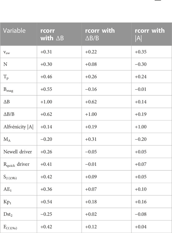
TABLE 1. Correlation coefficients between relevant variables and ΔB = <(B- <B>)2 > 1/2, ΔB/B, and Alfvénicity |A|. The Alfvénicity is calculated using the ACE data in the years 1998–2008, other correlations use the OMNI2 dat in the years 1998–2012.
Three key questions are as follows. 1) Is the fluctuation effect on geomagnetic activity real? 2) If it is real, by what mechanisms do the fluctuations affect the coupling of the solar wind to the magnetosphere? 3) Or, is the fluctuation amplitude a proxy for something else in the solar wind that affects the coupling? Prior publications on the fluctuation effect largely did not consider these three issues.
This paper is organized as follows. Section 2 contains new and improved data analysis of the connections between upstream fluctuation amplitudes, Alfvénicity, and geomagnetic activity. Section 3 summarizes the new statistical findings and draws conclusions. Section 4 discusses (a) the potential role of solar-wind current sheets and velocity shears, (b) the fluctuation effect in the different major types of solar-wind plasma, (c) a reconnection-clock-angle effect, and (d) a connection between the solar-wind driving of the magnetosphere and the standard model for MHD turbulence in the solar wind. Section 5 suggests needed future work to discern whether or not the upstream-fluctuation effect is real.
Figure 1 uses 1-hr-averaged OMNI2 data (King and Papitashvili, 2005) to demonstrate the suspected effect of upstream solar-wind fluctuations on the magnetosphere independent of the rate of dayside reconnection. Here the 1-hr-lagged (from the solar wind) AE index (AE1) is plotted as a function of the fluctuation amplitude ΔB/B in the upstream solar wind. ΔB/B is effectively the rms wiggle angle (in radians) of the magnetic-field direction averaged for that hour of solar-wind data. To gauge the magnitude of the dayside reconnection rate the function Rquick is used, where
(e.g., Borovsky and Birn, 2014; Borovsky and Yakymenko, 2017), where nsw is the solar-wind number density, mp is the proton mass, θclock is the (GSM) clock angle θclock = arccos (Bz/(By2+Bz2)1/2), and MA is the solar-wind Alfvén Mach number. Rquick was derived to be the solar-wind controlling factor for the reconnection rate at the nose of the dayside magnetopause. Each of the curves plotted in different colors in Figure 1 pertains to a subset of 10% of the data categorized into the subsets according to the magnitude of Rquick in each hour of data. For example, the dark-red curve at the bottom of the plot is for the times when the value of Rquick is in the lowest 10% of its values, the red curve is for the second lowest 10% of the Rquick values, the orange curve is for the third lowest 10% of the Rquick values, etc. Only the first six of the 10 intervals are plotted: the two highest-Rquick intervals have a trend that reverses in the plot. As the Rquick values increase from subset to subset in Figure 1, the dayside reconnection rate increases and the curves shift to higher values of AE1. In Figure 1 the individual hourly values of AE1 are not plotted, rather for each subset of data a 300-point running average of AE1 versus ΔB/B is plotted to show the underlying trend in the scatter of points. The Pearson linear correlation coefficient rcorr between AE1 and ΔB/B is indicated on the plot for each data subset: this rcorr value pertains to the individual hourly data points not to the running averages. In each data subset there are about 27,000 hourly data points so rcorr values that are |rcorr| > 0.012 are statistically significant (i.e., inconsistent with random). As can be seen in Figure 1, AE1 increases systematically with increasing amplitudes ΔB/B of upstream solar-wind fluctuations, whether or not dayside reconnection is expected on the basis of solar-wind conditions.
Figure 1 is similar to Figure 6 of Borovsky and Steinberg (2006b) where the solar-wind driver function vswBz was used to sort the data: Rquick used in Figure 1 is a superior variable to use for sorting the data according to the expected dayside reconnection rate.
The reversal of the ΔB/B correlation with AE1 for strong values of Rquick can be seen in the red curve with circular points in Figure 2 where correlation coefficients rcorr between several solar-wind variables and AE1 are plotted for each of the 10 bins of Rquick, with low values of Rquick to the left in the plot and large values of Rquick to the right. In Figure 2 attention should be paid to the Rquick bins to the left where the ΔB/B effect is not overwhelmed by the Rquick reconnection driving. Note that with this Rquick sorting there are other solar-wind variables that have higher correlation coefficients with AE1 than ΔB/B does: in particular nv2 (green curve) and vsw (dark-red curve). In constructing viscous-interaction driver functions that act in addition to dayside-reconnection driving, these two variables are prominent (Borovsky, 2013), including when an “eddy-viscosity” driver function is derived (cf. expression (2a) below). As can be seen in expressions (2a), (2b), and (2c) below, this derived eddy-viscosity driver function depends linearly on the amplitude of the solar-wind magnetic-field fluctuations ΔB, and also on various powers of the solar-wind number density and the solar-wind velocity and it depends on algebraic functions of the solar-wind Mach number and the angle between the solar-wind magnetic field and the Sun-Earth line.
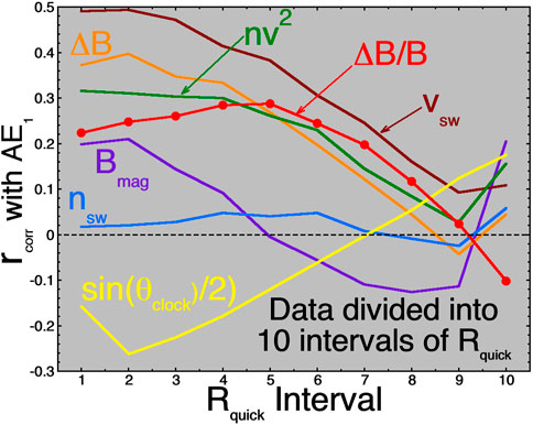
FIGURE 2. Correlation coefficients rcorr between several solar-wind variables and AE1 are plotted for each of the 10 bins of Rquick (binned as in Figure 1).
As stated above, for very large values of Rquick the AE-versus-ΔB/B trend reverses. For strong Rquick, the ΔB/B effect is a small fraction of the total driving and difficult to analyze: any effect that causes the strong reconnection rate to vary could dominate over the ΔB/B effect. Without specifically studying these cases, one can only speculate. The decrease at strong Rquick might be owed to the fact that the strong-driving cases sometimes involve magnetic clouds (often the strongest-driving times) and ΔB/B is small in clouds (e.g., Richardson and Cane, 2010): the selection of small ΔB/B in that case is then picking out strong driving by clouds.
The two panels of Figure 3 repeat the process of Figure 1, but sort on two other solar-wind variables besides Rquick. The left panel sorts the data into 10 bins of vsw values and the right panel sorts the data into 10 bins of ram pressure nv2 values. In both panels the relationship between ΔB/B and AE is much weakened from Figure 1 with correlation coefficients rcorr that are in general a small fraction of those in Figure 1 where Rquick sorting was used. This validates the interpretation of Figure 1 that the ΔB/B affect is in addition to the reconnection driving described by Rquick.
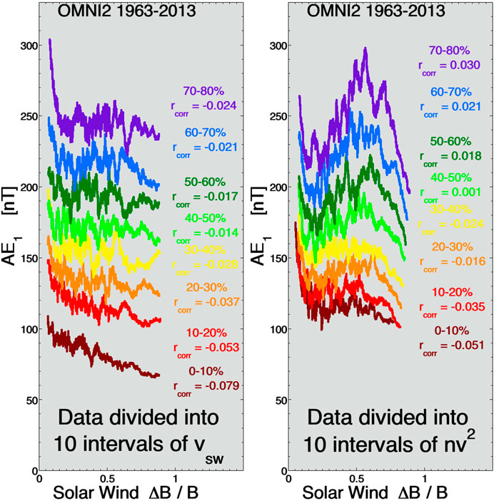
FIGURE 3. (left panel) For times when the value of vsw is in 10-percent intervals, 300-point running averages of the one-hour-lagged AE index is plotted as a function of the amplitude ΔB/B of the upstream solar-wind turbulence. (right panel) For times when the value of the solar wind ram pressure nv2 is in 10-percent intervals, 300-point running averages of the one-hour-lagged AE index is plotted as a function of the amplitude ΔB/B of the upstream solar-wind turbulence.
Figure 4 is similar to the plots of Figure 1, but a composite “Earth index” is used rather than a single geomagnetic index. The composite index E(1)(9a) is given by eq. (9a) of Borovsky and Denton (2014) and it is comprised from nine measures of magnetospheric activity: the standard geomagnetic indices AE, AU, AL, PCI, Kp, and Dst, plus a 1-hr-resolution midnight boundary index MBI (Gussenhoven et al., 1983), plus two ULF indices Sgrd and Sgeo (Borovsky and Denton, 2014). The mathematical method used to derive the composite index E(1)(9a) is canonical correlation analysis (CCA) and the method also derives a solar-wind driver function S(1)(9b) that corresponds to E(1)(9a). To make Figure 4, only times when the driver function S(1)(9b) is in its first (lowest) ten percentiles are used. The first 10% choice is for simplicity and is meant to sort for times when dayside reconnection is low. Then, for those times, a running average of E(1)(9a) as a function of ΔB/B is plotted. As can be seen, there is a clear trend where the Earth index E(1)(9a) systematically increases as the amplitude of the solar-wind fluctuations increases. For the hourly points used in Figure 4 (not the running average), the Pearson linear correlation coefficient rcorr between E(1)(9a) and ΔB/B is rcorr = 0.16, again a definite correlation.
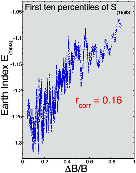
FIGURE 4. For times when the solar-wind composite driver function S(1)(9b) is in its lowest 10% of values, a 101-point running average of the Earth index E(1)(9a) is plotted as a function the upstream fluctuation amplitude ΔB/B.
Figure 5 is similar to Figure 1 but it uses only the lowest 10% of the Rquick values and it examines geomagnetic activity as functions of other non-reconnection solar-wind drivers. Again, the choice of the first 10% is for simplicity and is meant to sort for times when dayside reconnection is low. The blue curves replot AE1 [panel (a)] and Hp601 [panel (b)] as a function of ΔB/B for the upstream solar-wind fluctuations. (Hp60 is a 60-minute-resolution version of the Kp index now available at ftp://ftp.gfz-potsdam.de/pub/home/obs/Hpo; Hp601 is the Hp index lagged by 1 h from the solar-wind-at-Earth measurements.) Again running averages of the individual hourly points are plotted. The red curves in both panels of Figure 5 plot geomagnetic activity as a function of vsw for the times with the lowest 10% of Rquick values, with vsw intercorrelated with ΔB/B (cf. Table 1). The green curves in both panels of Figure 5 plot geomagnetic activity as a function of the Mach-number-dependent theoretical eddy-viscosity-based coupling coefficient F for the super-sonic solar wind [cf. Eqs. 4d, (61), and (63) of Borovsky (2013)]
where nsw is the solar-wind number density, vsw is the solar-wind speed,
where βs is the plasma-beta value of the magnetosheath plasma at the nose of the magnetopause. Simpler non-Mach-number dependent Bohm viscosity coefficients for non-super-sonic solar wind have been derived by Eviatar and Wolf (1968) and by Vasyliunas et al., (1982). Again, for F and B only the running averages are plotted in Figure 5. Note that the horizontal axis of Figure 5 has been approximately “normalized” for all variables ΔB/B, vsw, F, and B so that the running-average curves each extend from ∼0 to ∼1 for easy visual intercomparison. Figure 5 shows systematic increases in AE1 [panel (a)] and Hp601 [panel (b)] for increasing values of each of the drivers. Pearson linear correlation coefficients rcorr are also indicated for the hourly points in Figure 5. The significance levels for the correlation coefficients (with ∼15,600 hourly data points for each variable) is |rcorr| > 0.016. Recall that the data points used for Figure 5 were only the times when the Rquick values were in the lowest 10 percentiles, i.e., during weak dayside reconnection.
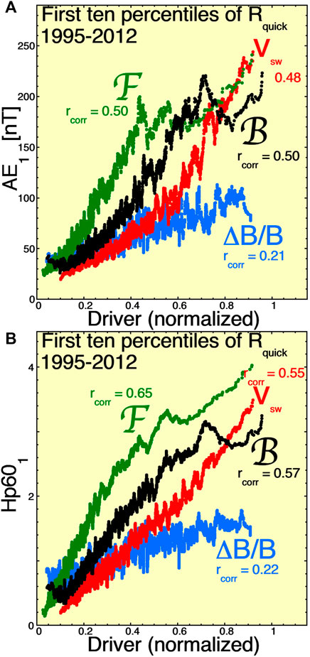
FIGURE 5. For times when the value of Rquick is in its lowest 10%, 101-point running averages of AE1 [panel (A)] and Hp601 [panel (B)] are plotted as functions of four “drivers”: ΔB/B (blue), vsw (red), F (green), and B (black).
Whereas in Figure 5 the variation of ΔB/B corresponds to an increase in AE1 of about 75 nT and to an increase of Hp601 of about 1, the other driver variables seem to account for much larger increases, about 200 nT in AE1 and up to 3.5 values of Hp601. The values of AE1 increase seem reasonable, but the values of Hp601 increase seem large if this is a “subtle” as-yet-unconfirmed driving mechanism. The Hp601 changes in Figure 5 are from ∼0.5 to ∼4; note that Hp60 is a logarithmic index so changes of Hp at small values of Hp involve smaller changes in activity than do changes of Hp at large values of Hp.
The effect of the solar-wind Alfvénicity is explored in Figures 6–10. The Alfvénicity |A| of the solar wind is calculated using measurements from the ACE spacecraft at L1 with 64-s averaged values from the Magnetic Field Instrument (MFI) (Smith et al., 1998) and proton flow measurements with 64-s time resolution from the Solar Wind Electron Proton Alpha Monitor (SWEPAM) (McComas et al., 1998), both data sets from the “Merged IMF and Solar Wind 64-s Averages” (available from the ACE Science Center at http://www.srl.caltech.edu/ACE/ASC/level2/index.html). The |A| value of the fluctuations for each hour of data at 128-s is calculated, where
with
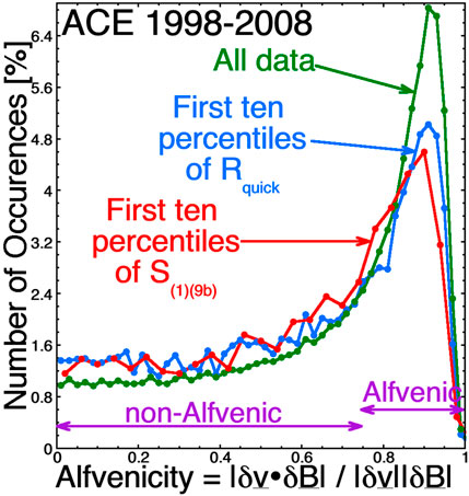
FIGURE 6. Occurrence distributions of the Alfvénicity |A| are plotted for all times (green), for times when the value of Rquick is in the lowest 10% of its values (blue), and for time when the value of S(1)(9a) is in the lowest 10% of its values.
Three occurrence distributions for the Alfvénicity |A| are plotted in Figure 6: for all times (green curve), for times when the Rquick values are low (the first ten percentiles) (blue curve), and for times when the solar-wind driver function S(1)(9b) is low (the first ten percentiles) (red curve). High Alfvénicity is high velocity-field correlation, so Alfvénic wind in Figure 6 will be taken as |A| > 0.75 and non-Alfvénic wind will be taken to be |A| < 0.75. As can be discerned by the distribution shapes of Figure 6, the Alfvenicity tends to be high (>75%) or modest (<75%). The Alfvenicity is rarely unity. The flat-shaped distribution of Alfvenicity values in Figure 6 (which should extend from |A| = 0 to |A| = 1) is consistent with uncorrelated (random, non-Alfvenic) values of δB and δv changes, i.e., non-Alfvenic regions of solar wind [cf. Figure 11B of Borovsky et al., (2019)].
In the two panels of Figure 7 the relation of Alfvénic wind (red curves) versus non-Alfvénic wind (blue curves) to geomagnetic activity as measured by the AE index [panel (a)] and by the Kp index [panel (b)] is explored. Data for all times in 1998–2008 is used. The individual hourly data points are not plotted: instead 201-point running averages of the individual hourly points are plotted to show the trends underlying the scatter of points. Pearson linear correlation coefficients rcorr for the hourly data points (not the running averages) are indicated on the plots. Both panels of Figure 7 indicate a change in the geomagnetic activity for weak driving (low Rquick values) between Alfvénic wind (red) and non-Alfvénic wind (blue), with elevated geomagnetic activity in the Alfvénic wind. A “relationship” between Alfvénicity and geomagnetic activity is seen, but an important question focuses on whether or not the relationship is cause and effect? One might worry because the Alfvénicity |A| of the solar wind is correlated with several other variables and a “correlative” relationship could be created by |A| acting as a proxy for a more-causal variable. In Table 1 some Pearson linear correlation coefficients between the Alfvénicity |A| and other solar-wind and magnetospheric variables are collected. Note in the solar wind a somewhat robust correlation of |A| with vsw (+0.35) and weaker correlations of |A| with ΔB and ΔB/B (+0.14 and +0.19). These positive correlations in part are probably associated with the high Alfvenicity of coronal-hole-origin plasma, which has tends to have high velocities [cf. Figures 8, 11 of Borovsky et al., (2019)].
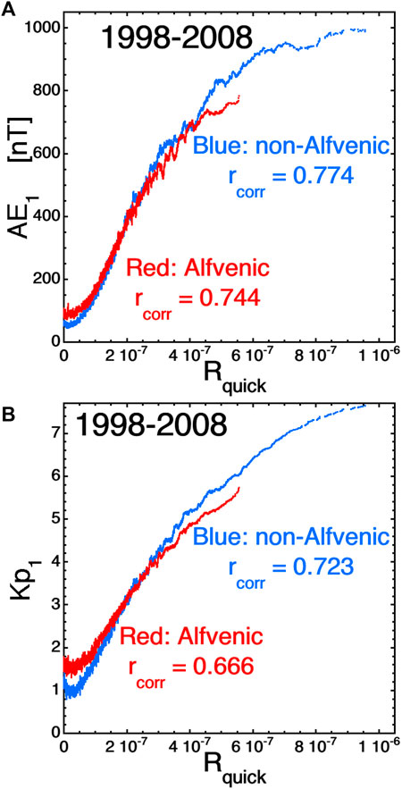
FIGURE 7. 201-point running averages of AE1 [panel (A)] and of Kp1 [panel (B)] are plotted as functions of the solar-wind driver Rquick separately for times when the solar wind was non-Alfvénic (blue, |A| < 0.75) and for times when the solar wind was Alfvénic (red, |A| > 0.75).
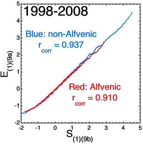
FIGURE 8. 201-point running averages of the Earth index E(1)(9a) are plotted as functions of the solar-wind composite driver S(1)(9b) separately for times whe n the solar wind was non-Alfvénic (blue, |A| < 0.75) and for times when the solar wind was Alfvénic (red, |A| > 0.75).
In Figure 8 the relation of Alfvénic wind (red curve) versus non-Alfvénic wind (blue curve) to geomagnetic activity as measured by the E(1)(9a) composite magnetospheric-activity index is explored. As in the prior figures, the individual hourly data points are not plotted: instead a 201-point running average of the individual hourly E(1)(9a) values are plotted to show the trends underlying the scatter of points. Pearson linear correlation coefficients rcorr for the hourly data points (not the running averages) are indicated on the plot. Contrary to AE and Kp in Figure 7, there is very little systematic difference between the values of E(1)(9a) for Alfvénic versus non-Alfvénic solar wind. At this point, no explanation for the reduced effect on E(1)(9a) is available: two inconclusive research efforts intersect on this point. 1) In the present research the effect of solar-wind fluctuations is being examined and 2) in other active research efforts (e.g., Borovsky and Denton, 2018; Borovsky and Osmane, 2019; Borovsky, 2021b) the properties of the composite index are being examined, with no full understanding on either issue.
Figure 9 is similar to Figure 5 using the lowest 10% of the Rquick values, examining geomagnetic activity as measured by AE [panel (a)] and Hp60 [panel (b)] as functions of the value of the Alfvénicity |A| for the weak Rquick driving of the magnetosphere. Again running averages of the individual hourly points are plotted. Both panels of Figure 8 indicate increases in geomagnetic activity associate with Alfvénic wind (|A| > 0.75), with almost 100 nT of AE increase and about half a unit of Hp60 increase. For the times when the Rquick value is in the lowest 10%, the Pearson linear correlation coefficient rcorr between |A| and the two geomagnetic indices are indicted on the two plots of Figure 9.
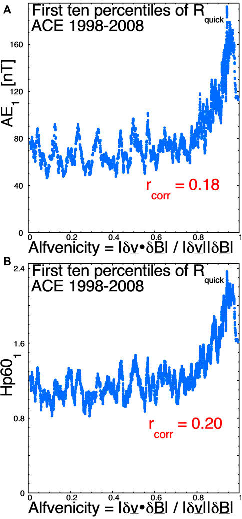
FIGURE 9. For times when the solar-wind driver Rquick is in its lowest 10% of values, 101-point running averages of AE1 [panel (A)] and of Hp601 [panel (B)] are plotted as functions of the Alfvénicity |A|.
Figure 10 is similar to Figure 9, but it looks at the effect of the solar-wind Alfvénicity |A| on the composite magnetospheric-activity index E(1)(9a) when the magnetospheric driving by the solar-wind variable S(1)(9b) is at its lowest 10% of values. A distinct relation is seen in Figure 10 between Alfvénic wind (|A| > 0.75) and an increase in E(1)(9a), but compared with the vertical range of values of E(1)(9a) seen in Figure 8, the ∼0.15 increase in E(1)(9a) is quite small. The correlation between |A| and E(1)(9a) for the lowest 10% of S(1)(9b) driving is also quite weak (+0.05).
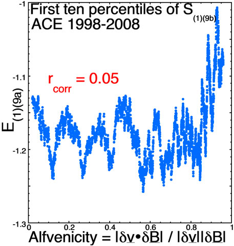
FIGURE 10. For times when the solar-wind composite driver S(1)(9b) is in its lowest 10% of values, 101-point running averages of the Earth index E(1)(9a) is plotted as a function of the Alfvénicity |A|.
Figure 11 explores the combined effects of ΔB/B and Alfvénicity |A|. For times when the value of Rquick is in the lowest 20% of its values, the 1-h lagged AE1 index and the 1-h-lagged Hp601 index are binned according to the values of ΔB/B and the Alfvénicity |A| in each hour of data. Figure 11A denotes the mean value of AE1 in each bin: red (AE1 > 100 nT), yellow (75 < AE1 < 100), green (50 < AE1 < 75), and blue (AE1 < 50 nT). Figure 11B denotes the mean value of Hp601 in each bin: red (Hp601 > 2), yellow (1.5 < Hp601 < 2), green (1 < Hp601 < 1.5), and blue (Hp601 < 1). Both large ΔB/B and strong |A| seem geoeffective: the highest activity levels are approximately in the upper-right corners of the plots where ΔB/B and |A| are largest. The two plots seem to indicate that stronger geomagnetic activity can occur for strong ΔB/B, even if |A| is weak. However, the opposite is not true: if ΔB/B is weak there is no strong activity if |A| is weak. The interpretation of Figure 11 is not definitive, but it seems to indicate that ΔB/B is more important than Alfvénicity for driving geomagnetic activity.
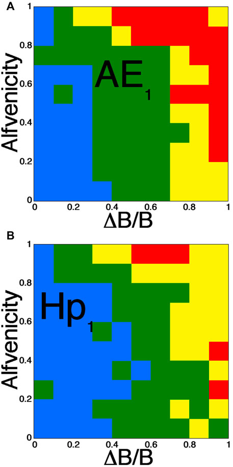
FIGURE 11. For times when Rquick is in the lowest 20% of its values, the AE index and the Hp60 index are binned according to the values of ΔB/B and the Alfvénicity |A|. Panel (A) denotes the mean value of AE1 in each bin: red (AE1 > 100 nT), yellow (75 < AE1 < 100) green (50 < AE1 < 75), and blue (AE1 < 50 nT). Panel (B) denotes the m an value of Hp601 in each bin: red (Hp601 > 2), yellow (1.5 < Hp601 < 2), green (1 < Hp601 < 1.5), and blue (Hp601 < 1).
There are three key questions. 1) Is the fluctuation effect on geomagnetic activity real? 2) If it is real, by what mechanisms do the fluctuations affect the coupling of the solar wind to the magnetosphere? 3) Or, is the fluctuation amplitude a proxy for something else in the solar wind that affects the coupling? Related to question 2) are two further questions: (A) do the solar-wind fluctuations change the dayside reconnection rate? or (B) do the solar-wind fluctuations create or enhance a viscous coupling of the solar wind to the magnetosphere?
In this report statistical data-analysis evidence is gathered that is consistent with an effect of the amplitude of solar-wind magnetic-field fluctuations on geomagnetic activity, supporting a number of prior studies. This report also gathers statistical data-analysis evidence consistent with a connection between the Alfvénicity of solar-wind fluctuations and geomagnetic activity, supporting prior studies. Evidence that argues against a change-in-dayside-reconnection-rate effect is 1) an effect of the amplitude of fluctuations on geomagnetic activity for strongly northward IMF in the studies of Borovsky and Funsten (2003), Borovsky and Steinberg (2006b), Borovsky (2006), and Osmane et al., (2015) and 2) the effect of the amplitude of fluctuations on geomagnetic activity for very weak values of Rquick throughout the present study. On this second issue (Rquick being weak) there are two worries. First, Rquick is not a perfect description of the control of geomagnetic activity by the solar wind. For instance, in Figure 7A the linear correlations between Rquick and AE1 are rcorr ∼ 0.75, so the amount of variation of AE1 not described by a knowledge of the Rquick value is 1 - rcorr2 = 44%. Second, Rquick can change quickly mostly owing to frequent clock-angle changes and there is persistence to geomagnetic activity (cf. Lockwood, 2022), so an hour of weak Rquick could have been preceded by an hour of strong Rquick and the geomagnetic activity from that prior hour of driving could still persist. When ΔB/B is larger, temporal changes in Rquick are likely to be larger (Note that the analysis of Figure 5 of Borovsky and Steinberg (2006b) attempted to guard against this persistence phenomenon and when persistence was eliminated the relationship between ΔB/B on geomagnetic activity was lessened.).
The Bohm-viscosity driver function B without direct information about the fluctuation amplitudes ΔB does about as good a job as does the freestream-turbulence driver function F that contains information about ΔB, as seen by comparing the black and green curves in each of the two panels of Figure 5. This might be an indication of a proxy effect for ΔB/B.
In the present data analysis the effect of the fluctuation amplitudes ΔB/B on the composite whole-magnetosphere activity index E(1)(9a) is found to be small compared to the effect of ΔB/B on AE or Kp. There is no idea as to why. The driver function S(1)(9b) used in the present data-analysis study does not have direct information in it about ΔB (cf. eq. (9b) of Borovsky and Denton (2014)). Note that in other constructions of composite solar-wind driving functions using the CCA methodology, if the ΔB variable is offered to the process it will be accepted into the solar-wind driving function S(1); examples are eq. (14) of Borovsky (2014) and Eq. 1b of Borovsky and Osmane (2019). Interpreting the CCA process, the acceptance of the ΔB variable indicates that it may carry unique information that is needed to better describe geomagnetic activity in terms of solar-wind variables.
In summary, evidence is found that supports definitive relationships 1) between the solar wind ΔB/B and geomagnetic activity and 2) between solar-wind Alfvénicity and geomagnetic activity. The ΔB/B relationship seems to be stronger than the Alfvénicity relationship. No clear evidence is found that precludes these relationships from being physical cause-and-effect, although that is still an outstanding question. Needed future work is discussed in Section 5: meanwhile researchers should be cautious.
The potential roles of solar-wind current sheets, the coupling in different types of solar-wind plasma, and the role of averaging of solar-wind magnetic clock angles are discussed.
The amplitude measure ΔB of the magnetic-field fluctuations in the upstream solar wind is dominated by the ubiquitous strong current sheets (discontinuities) in the solar-wind plasma (Siscoe et al., 1968; Borovsky, 2010); the amplitude measure ΔB does not represent randomly-phased waves (or eddies) at diverse wavelengths (Borovsky, 2022b). The magnetic-field Fourier power spectral density (amplitude and shape) of the solar wind reflects the properties (sizes, occurrence distribution, thickness, and thickness profile) of the solar-wind current sheets [cf. Table 1 of Borovsky and Burkholder (2020)]. The strong current sheets have thicknesses of about 1,000 km (Vasquez et al., 2013) and pass the Earth at a rate of several per hour (Borovsky, 2008b); their orientations are such that the normals to the current sheets tend to be perpendicular to the Parker-spiral direction (Borovsky, 2008b). If the current sheets are not time resolved in the time series, the time series still contains the information about the jump sizes in vector-B across the current sheets and about the temporal occurrence distribution of the current sheets. In Figure 3 of Borovsky (2010) it is demonstrated that the Fourier power (amplitude) of the solar wind at frequencies lower than the time resolution is captured by using only 64-s information about the properties (size and occurrence distribution) of the current sheets seen in the ACE 64-s data for 9 years of measurements. This is the amplitude of ΔB that OMNI2 contains in its ΔB values, which are the fluctuation amplitudes for every UT hour measured with a time resolution that is a small fraction of an hour. Hence, OMNI2 contains a proper measurement of the amplitude of solar-wind fluctuations driven by the solar-wind current sheets. If the current sheets are fully time resolved in the measurements, then the Fourier power above the first high-frequency Fourier breakpoint is captured, in addition to the lower-frequency Fourier amplitude in the inertial range. This capture of high-frequency power when current sheets are resolved is demonstrated in Figures 7, 8 of Borovsky and Podesta (2015) and in Figure 11 of Borovsky and Burkholder (2020).
It is worth speculating whether the passages of the strong current sheets have an impact on the net driving of the Earth’s magnetosphere by the solar wind. It is well known that some solar-wind current sheets can produce dayside transients as the current sheets encounter the Earth’s bow shock [e.g., Sibeck et al., 1999; Sibeck et al., 2000; Zesta and Sibeck, 2004]. The passage of a strong current sheet represents a sudden strong change in the orientation of the solar-wind magnetic-field vector: this produces a temporal “on-off” driving of the magnetosphere via dayside reconnection. A question is: does the on-off driving produce a stronger overall coupling than does steady driving? The change in the reconnecting IMF can produce a twist to the magnetosphere requiring a re-orientation of some magnetospheric current systems. A second question is: does the suddenness of the changes between on-off driving result in enhanced overall coupling? The sudden change of the magnetic-field orientation across a current sheet also produces a sudden change in the IMF clock angle θclock and a shift in the level of driving via dayside reconnection and probably a change in the location of the reconnection site on the dayside magnetopause. A third question is whether jumps in the location of the dayside reconnection site somehow results in enhanced overall coupling? Arguments against these three speculations lie in the fact that the ΔB/B effect persists under strongly northward IMF when there should be little reconnection between the solar wind and the magnetosphere.
Solar-wind strong current sheets (which drive the amplitude of the measured solar-wind magnetic-field fluctuations) are often accompanied by intense abrupt velocity shears, particularly in the “Alfvénic” solar wind. The Alfvénicity measure of the solar wind |A| = |δv•δB/|δv||δB| is also dominated by the strong current sheets (“discontinuities”) of the solar wind and their co-located strong velocity shears [cf. Figure 12 of Borovsky and Denton (2010)]. The impacts of intense velocity shears on the magnetosphere have been investigated by Borovsky (2012a), Borovsky (2018c) via data analysis and global MHD computer simulations. A common feature seen in the global simulations are comet-like disconnections of the Earth’s magnetotail, although these are not likely to produce an enhanced coupling as seen in geomagnetic indices. Other effects seen in the global simulations (Borovsky, 2012a) are temporary enhancements or decreases in the cross-polar-cap potential, the production of ULF waves interior to the magnetosphere, and abrupt changes in the wind-sock orientation of the magnetosphere.
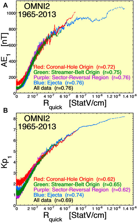
FIGURE 12. Geomagnetic activity is plotted as a function the reconnection driver function Rquick separately for the four types of solar-wind plasma. Panel (A) plote AE1 and panel (B) plots Kp1. Only running averages of the individual hourly data points are plotted.
In general Δv is strongly correlated with ΔB in the solar wind [e.g., Figure 14 of Borovsky (2012b)] and particularly in the Alfvénic coronal-hole-origin plasma Δv/vA (where vA is the Alfvén speed of the solar wind) is highly correlated with ΔB/B [e.g., Figure 13B of Borovsky and Denton (2010)]. Hence, it is undoubtedly true that geomagnetic activity is correlated with Δv and Δv/vA of the solar wind. Future studies should explore the connection between the solar-wind velocity-fluctuation amplitude and geomagnetic activity.
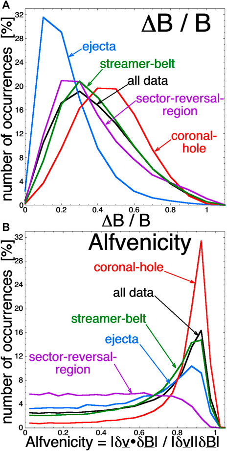
FIGURE 13. The occurrence distribution of ΔB/B [panel (A)] and Alfvénicity |A| [panel (B)] are plotted for the four types of solar-wind plasma.
Xu and Borovsky (2015) developed a categorization scheme at one AU that separates the solar wind at 1AU into four types, depending on the regions of the solar surface from which the different plasma types originate. The four types are coronal-hole-origin plasma, streamer-belt-origin plasma, sector-reversal-region plasma, and ejecta. The four types of solar wind have systematically different properties, including the properties of the magnetic-field and velocity fluctuations in the plasmas (Xu and Borovsky, 2015; Borovsky et al., 2019). Figure 12 plots geomagnetic activity as a function of the reconnection driver function Rquick as given by expression 1): in panel (a) geomagnetic activity is measured with the 1-h-lagged AE index and in panel (b) geomagnetic activity is measured with the 1-h lagged Kp index. For the plots of Figure 12, the 1-hr-resolution OMNI2 data was separated into the four categories of solar-wind plasma and a 101-point running averages of the data for each type is plotted. Both panels of Figure 12 show a trend that for weak reconnection driving (low values of Rquick) coronal-hole-origin plasma (red curves) exhibits higher levels of geomagnetic activity than do the other types of plasma. The four types of plasma have systematically different properties: as noted in Table 5 of Xu and Borovsky (2015) and Table 1 of Borovsky et al., (2019): coronal-hole-origin plasma tends to have higher values of the solar-wind speed vsw, lower values of the solar-wind number density nsw, higher values of the magnetic-field-vector fluctuation amplitude ΔB/B, higher values of the flow-vector fluctuation amplitude Δv/vA, and higher values of the Alfvénicity |A|. The occurrence distributions of ΔB/B [panel (a)] and Alfvénicity |A| [panel (b)] are shown in Figure 13 separately for the four types of solar-wind plasma: the elevated values of ΔB/B and |A| for coronal-hole-origin plasma (red curves) are clearly seen. In Figure 12A at low driving (low Rquick values), the mean AE1 values of the coronal-hole-origin plasma are about 60 nT larger than they are for the three other plasma types. In Figure 13A, the median ΔB/B value of coronal-hole-origin plasma is 0.443 and for all other plasma types combined the median value is 0.315, meaning that ΔB/B is increased by about 0.128 for coronal-hole-origin plasma. In Figure 1 for weak driving (lower curves), an increase of ΔB/B by about 0.13 would correspond to an increase of AE by only about 10 nT. This sheds doubt on the increase of AE (and Kp) for low driving in the two panels of Figure 12 being caused by a systematic increase in the fluctuation amplitude in coronal-hole-origin plasma. If one zooms in on the low-driving portions of the plots in the two panels of Figure 12 one finds that geomagnetic activity, as measured by both AE and Kp, increases systematically from sector-reversal-region plasma (purple), to streamer-belt-origin plasma (green), to ejecta (blue), to coronal-hole-origin plasma (red): one solar-wind variable that systematically increases in that order from plasma type to plasma type is the solar-wind speed vsw (cf. Figure 8C of Xu and Borovsky (2015) and Figure 2A of Borovsky et al., (2019) with the same color scheme). As noted in Table 1, ΔB/B is positively correlated with vsw and the correlation of geomagnetic activity with ΔB/B could be a proxy for a cause-and-effect correlation between vsw and geomagnetic activity in addition to the driving described by Rquick, which is itself a function of vsw. Here, the use of information transfer (cf. Section 5) may be able to discern causal versus correlative connections between the two solar-wind variables ΔB/B and vsw versus geomagnetic activity.
The dayside reconnection rate is thought to vary as sina (θclock/2) where the exponent a = 2 in the Rquick driver function (Borovsky and Birn, 2014) and a = 8/3 in the Newell driver function (Newell et al., 2007). For various geomagnetic indices the optimal value of the exponent a varies (Borovsky, 2022c). A question is: does the time-variable clock angle θclock produce a stronger overall coupling than does steady driving? This is examined in Figure 14, where steady driving with a steady clock angle of 90° (Parker-spiral orientation at the solstice) is compared with a sinusoidally varying clock angle that varies with time t as 90° + 45osin(t). In Figure 14 sin (θclock/2), sin2 (θclock/2), and sin3 (θclock/2) are each plotted as a function of time for the steady 90° clock angle (flat lines) and for the sinusoidally oscillating clock angle. In the black-font table in Figure 14 the time averages of these quantities is listed. As can be seen in Figure 14 the average value of the clock angle θclock is the same for the steady 90° angle as it is for the sinusoidally varying angle. As can be seen in Figure 14 (and the table within) the average value of sin (θclock/2) (blue curves) is lower for the sinusoidally varying clock angle than it is for the steady clock angle. For sin2 (θclock/2) (red curves in Figure 14) the time-averaged value is the same for the steady and the varying clock angle. For sin3 (θclock/2) (green curves in Figure 14) the time-varying clock angle yields a larger mean value than does the steady clock angle. Hence, if the physical reconnection driver function has a dependence sina (θclock/2) with exponent a >2, then one could expect the fluctuations in the solar-wind clock angle to produce an enhanced solar-wind reconnection coupling than would a steady clock angle, giving one possible explanation to the observed statistical increase of coupling with an increase in the amplitude of upstream solar-wind magnetic fluctuations. In this case the enhanced coupling driven by the solar-wind fluctuations would be an enhanced average dayside reconnection rate. The Newell coupling function has sin8/3 (θclock/2), which would result in an enhance coupling with fluctuations; the Rquick coupling functions has sin2 (θclock/2) which would not result in an enhanced coupling with fluctuations.
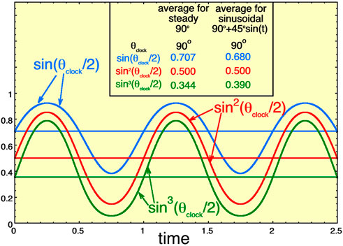
FIGURE 14. The functions sin(θclock/2) (green), sin2(θclock/2) (red), and sin3(θclock/2) (blue) are plotted as functions of time for the steady 90o clock angle and for the sinusoidally oscillating clock angle 90o + 45osin(t). The table in the figure lists the average values for the steady 90o clock angle and for the sinusoidal 90o + 45osin(t) clock angle.
When considering this clock-angle effect, it must be kept in mind that the amplitude of the ΔB/B effect persists under strongly northward IMF [e.g., Figure 4 of Borovsky and Funsten (2003) or Figure 5 of Borovsky and Steinberg (2006a), Borovsky and Steinberg (2006b)] where dayside reconnection should be a very weak effect and modulating it should not produce much geomagnetic-activity change. The fact that the baseline level of geomagnetic activity is low when Rquick is low (cf. the dark-red, red, and orange curves in Figure 1) confirms that there is very little reconnection driving when θclock ∼ 0° (strongly northward).
In previous publications this is enhanced-geomagnetic-activity affect was referred to as a “turbulence” effect (e.g., Borovsky and Funsten, 2003; Borovsky and Steinberg, 2006b; Borovsky, 2006; Jankovicova et al., 2008a; Jankovicova et al., 2008b; D’Amicis et al., 2007; D’Amicis et al., 2009; D’Amicis et al., 2010; D’Amicis et al., 2020). As noted in Section 4.1 the measured amplitudes of ΔB in the solar wind are primarily owed to strong current sheets in the solar wind, with several sheets passing a spacecraft per hour. The origin of those current sheets is not understood (Neugebauer and Giacalone, 2010; Neugebauer and Giacalone, 2015; Li and Qin, 2011; Owens et al., 2011; Tu et al., 2016; Telloni et al., 2016; Viall and Borovsky, 2020): some could be associated with active turbulence (Greco et al., 2009; Zhdankin et al., 2012; Vasquez et al., 2013) but it is known that some are fossils from the corona (Borovsky, 2020b; Borovsky, 2021c; Borovsky and Raines, 2022). In this report the author chose to focus on the term “fluctuations” rather than “turbulence”.
If the fluctuations in the solar wind are purely turbulence, then the ΔB/B effect analyzed here would have an interesting interpretation. The “standard model” for MHD turbulence in the solar wind (based on the shape of the magnetic power spectral density plot for the solar wind) is that energy in large scale-scale passive structures feeds the turbulence cascade (Matthaeus et al., 1994; Matthaeus et al., 2015). The magnetic power spectral density of the solar wind typically has a mild breakpoint at a frequency of about 1 h (Tu and Marsch, 1995; Bruno et al., 2019). In the standard model lower-frequency power (1 h and longer) is attributed to the passive “energy-containing” scales and higher frequency power (1 h and shorter) is denoted as the “inertial range” of active turbulence. When hourly averaging the solar wind data, the hourly-averaged data describes the energy-containing structure: when looking at ΔB/B measured during 1 h one is looking at the inertial range fluctuations. Hence, from a turbulence point of view, an interpretation of the ΔB/B effect is that the Rquick driving is a driving of the Earth by the energy-containing structures in the solar wind and the additional ΔB/B geomagnetic activity represents driving of the Earth by active solar-wind turbulent fluctuations. Getting away from a turbulence point of view one could say that the Rquick driving is owed to larger-scale structure in the solar wind and that the ΔB/B effect is owed to the ubiquitous strong current sheets within that structure.
A number of mechanisms have been suggested for upstream solar-wind fluctuations to act to increase the coupling of the solar wind to the Earth’s magnetosphere: 1) reconnection with the southward-IMF portion of fluctuations (Tsurutani and Gonzalez, 1987; Tsurutani et al., 1999), 2) patchy magnetopause reconnection (Voros et al., 2002), 3) fluctuations increase favorable geometry for dayside reconnection (Jankovicova et al., 2008a; Jankovicova et al., 2008b), 4) fluctuations produce a global-scale eddy viscosity (Borovsky and Funsten, 2003; Borovsky, 2013), 5) current sheets or velocity shears play a role (suggested in Section 4.1), and 6) averaging of fluctuating sinx (θclock/2) functions suggested in Section 4.3). An alternative explanation is that the fluctuation amplitude acts as a proxy for some other more-relevant solar-wind variable. This presents an outstanding problem for space physics.
Further advancements in computer simulations are needed to help quantify and understand the effect of upstream solar-wind fluctuations on the Earth’s magnetosphere. These simulations can be local (focusing on perhaps one region around the magnetopause) or global, encompassing the upstream solar wind, the bow shock and magnetosheath, and the entire magnetosphere and magnetotail. Localized kinetic simulations indicate that the presence of magnetic-field fluctuations can lead to an enhanced growth of Kelvin-Helmholtz waves on the magnetopause (Nakamura et al., 2020), presumably producing a stronger coupling of the solar wind to the Earth’s magnetosphere. Adding Alfvénic fluctuations to the upstream solar wind in global MHD simulations of the magnetosphere found that ULF waves could be driven inside the magnetosphere McGregor et al., (2014): certainly if geomagnetic activity were to be measured by a ULF index (e.g., Romanova et al., 2007; Kozyreva et al., 2007; Romanova and Pilipenko, 2009), an increase in geomagnetic activity associated with the added Alfvénic fluctuations would be seen in the simulation. For solar-wind-fluctuation coupling studies, global MHD simulations have good aspects and bad aspects. Two good aspects are that the simulations can analyze the reaction of the global coupled magnetospheric system to the solar wind and that the simulations can correctly account for multiple simultaneous timelags for the diverse reactions. A bad aspect is the fact that MHD simulations can be dominated by high-derivative numerical errors at steep boundaries such as the magnetopause [cf. eq. (23) of Raeder (2003) or cf. Sect. 37.3 of Raeder et al., (2021)]. and at those critical locations physical conservation laws can be violated. This is not a resolution problem: it happens at the ideal-MHD grid scale whatever that scale is. This numerical-error problem leads to coupling related questions such as: Is the reconnection rate correct in the simulation? Are the viscous mechanisms correct in the simulation? Are the plasma-entry mechanisms correct in the simulation? Another drawback to present-day global MHD simulations is that the spatial resolution in the solar-wind portions of the simulation domain are very coarse so that small-spatial-scale (higher-frequency) solar-wind fluctuations cannot be included in the simulations. The field of solar-wind/magnetosphere coupling research looks forward to higher-Reynolds-number global-MHD simulations and to much-needed advancements in global hybrid and global Vlasov simulation methods.
Going beyond correlation studies with the use of information theory (information transfer, transfer entropy, etc.) is clearly a pathway that needs to be utilized in the future (e.g., March et al., 2005; Materassi et al., 2011; Balasis et al., 2013; Wing et al., 2016; Runge et al., 2018; Wing and Johnson, 2019; Manshour et al., 2021). For the outstanding question of whether or not the observed relationships between the solar-wind fluctuations and geomagnetic activity are cause-and-effect relationships, information theory can provide critical and more-clear evidence than simple correlations do.
As pointed out by D’Amicis et al., (2007), D’Amicis et al., (2009), D’Amicis et al., (2010) in regard to the relationship between solar-wind fluctuations and geomagnetic activity, there are different types of solar-wind fluctuations such as Alfvén waves, convected magnetic structures, MHD turbulence, etc. The work by D’Amicis et al., (2007), D’Amicis et al., (2009), D’Amicis et al., (2010) (and the work in the present study) of sorting Alfvénic versus non-Alfvénic wind for the coupling studies is a starting point for sorting the solar-wind data according to the type of fluctuations. In future, this sorting could be further progressed by inspection of the solar-wind time series and categorizing individual structures as they pass the solar-wind monitor.
Related to the sorting of the fluctuation type, it is recommended that analysis and thinking be focused on the specific effects of solar-wind current sheets and solar-wind velocity shears on geomagnetic activity. As noted in the discussion of Section 4, 1) the magnetic-field fluctuation-amplitude measure of the solar wind and 2) the Alfvénicity measure of the solar wind are both dominated by the ubiquitous strong current sheets of the solar wind.
A leading candidate mechanism underlying the viscous interaction is the Kelvin-Helmholtz instability on the Earth’s magnetopause (Miura, 1997; Nykyri and Otto, 2001; Masson and Nykyri, 2018) transporting magnetosheath momentum into the magnetosphere, transporting magnetosheath plasma into the magnetosphere, and enhancing reconnection between solar-wind magnetic-field lines and magnetospheric field lines. The “effective diffusion coefficient” related to the Kelvin-Helmholtz non-linear phase is able to explain the mass transport in different IMF configurations and taking into account the complex three-dimensional dynamics at the magnetopause (cf. Nakamura and Daughton, 2014; Borgogno et al., 2015; Sisti et al., 2019; Nykyri et al., 2021; Nakamura et al., 2022). It has been argued that the growth rate and effectiveness of the Kelvin-Helmholtz instability is enhanced when the level of velocity fluctuations in the magnetosheath is higher (Nykyri et al., 2017), and the level of fluctuations in the magnetosheath may be related to the level in the upstream solar wind. An investigation of the impact of solar-wind current sheets and their abrupt velocity shears on the Kelvin-Helmholtz physics might be fruitful.
Publicly available datasets were analyzed in this study. This data can be found here: https://omniweb.gsfc.nasa.gov.
JB performed all work for this project and wrote the manuscript.
The author thanks Gian Luca Delzanno, Chuck Smith, and Simon Wing for useful conversations. The author also acknowledges GFZ Potsdam for the Hp60 index, which is available at ftp://ftp.gfz-potsdam.de/pub/home/obs/Hpo, and the author acknowledges the SuperMAG team, where the SuperMAG auroral-electrojet indices are available at http://supermag.jhuapl.edu/indices.
The author declares that the research was conducted in the absence of any commercial or financial relationships that could be construed as a potential conflict of interest.
All claims expressed in this article are solely those of the authors and do not necessarily represent those of their affiliated organizations, or those of the publisher, the editors and the reviewers. Any product that may be evaluated in this article, or claim that may be made by its manufacturer, is not guaranteed or endorsed by the publisher.
Balasis, G., Donner, R. V., Potirakis, S. M., Runge, J., Papadimitriou, C., Daglis, I. A., et al. (2013). Statistical mechanics and information-theoretic perspectives on complexity in the Earth system. Entropy 15, 4844. doi:10.3390/e15114844
Blair, M. F. (1983a). Influence of free-stream turbulence on turbulent boundary layer heat transfer and mean profile development part 1: Experimental data. J. Heat. Transf. 105, 33.
Blair, M. F. (1983b). Influence of free-stream turbulence on turbulent boundary layer heat transfer and mean profile development, part II, Analysis of results. J. Heat. Transf. 105, 41–47. doi:10.1115/1.3245557
Borgogno, D., Califano, F., Faganello, M., and Pegorado, F. (2015). Double-reconnected magnetic structures driven by Kelvin-Helmholtz vortices at the Earth's magnetosphere. Phys. Plasmas 22, 032301. doi:10.1063/1.4913578
Borovsky, J. E., and Birn, J. (2014). The solar-wind electric field does not control the dayside reconnection rate. J. Geophys. Res. 119, 751–760. doi:10.1002/2013ja019193
Borovsky, J. E., and Burkholder, B. L. (2020). On the Fourier contribution of strong current sheets to the high-frequency magnetic power spectral density of the solar wind. J. Geophys. Res. 125, e2019JA027307. doi:10.1029/2019ja027307
Borovsky, J. E. (2014). Canonical correlation analysis of the combined solar-wind and geomagnetic-index data sets. J. Geophys. Res. 119, 5364–5381. doi:10.1002/2013ja019607
Borovsky, J. E. (2010). Contribution of strong discontinuities to the power spectrum of the solar wind. Phys. Rev. Lett. 105, 111102. doi:10.1103/physrevlett.105.111102
Borovsky, J. E., and Denton, M. H. (2018). Exploration of a composite index to describe magnetospheric activity: Reduction of the magnetospheric state vector to a single scalar. J. Geophys. Res. 123, 7384–7412. doi:10.1029/2018ja025430
Borovsky, J. E., and Denton, M. H. (2014). Exploring the cross-correlations and autocorrelations of the ULF indices and incorporating the ULF indices into the systems science of the solar-wind-driven magnetosphere. J. Geophys. Res. 119, 4307–4334. doi:10.1002/2014ja019876
Borovsky, J. E., Denton, M. H., and Smith, C. W. (2019). Solar wind turbulence and shear: A superposed-epoch analysis of corotating interaction regions at 1 AU. J. Geophys. Res. 124, 2406. doi:10.1029/2009ja014966
Borovsky, J. E., and Denton, M. H. (2010). Solar-wind turbulence and shear: A superposed-epoch analysis of corotating interaction regions at 1 AU. J. Geophys. Res. 115, A10101. doi:10.1029/2009ja014966
Borovsky, J. E. (2006). Eddy viscosity and flow properties of the solar wind: Co-Rotating interaction regions, coronal-mass-ejection sheaths, and solar-wind/magnetosphere coupling. Phys. Plasmas 13, 056505. doi:10.1063/1.2200308
Borovsky, J. E., and Funsten, H. O. (2003). Role of solar wind turbulence in the coupling of the solar wind to the Earth's magnetosphere. J. Geophys. Res. 108, 1246. doi:10.1029/2002ja009601
Borovsky, J. E. (2018c). Looking for evidence of wind-shear disconnections of the Earth’s magnetotail: GEOTAIL measurements and LFM MHD simulations. J. Geophys. Res. 123, 5538–5560. doi:10.1029/2018ja025456
Borovsky, J. E. (2022c). Noise and solar-wind/magnetosphere coupling studies: Data, submitted to Front. Astron. Space Sci. 9, 990789. doi:10.3389/fspas.2022.990789
Borovsky, J. E. (2022b). Noise, regression dilution bias, and solar-wind/magnetosphere coupling studies. Front. Astron. Space Sci. 9, 867282. doi:10.3389/fspas.2022.867282
Borovsky, J. E. (2018b). On the origins of the intercorrelations between solar wind variables. J. Geophys. Res. 123, 20–29. doi:10.1002/2017ja024650
Borovsky, J. E. (2021b). On the saturation (or not) of geomagnetic indices. Front. Astron. Space Sci. 8, 740811. doi:10.3389/fspas.2021.740811
Borovsky, J. E., and Osmane, A. (2019). Compacting the description of a time-dependent multivariable system and its multivariable driver by reducing the state vectors to aggregate scalars: The Earth's solar-wind-driven magnetosphere. Nonlin. Process. Geophys. 26, 429–443. doi:10.5194/npg-26-429-2019
Borovsky, J. E. (2021a). Perspective: Is our understanding of solar-wind/magnetosphere coupling satisfactory? Front. Astron. Space Sci. 8, 634073. doi:10.3389/fspas.2021.634073
Borovsky, J. E. (2013). Physics based solar-wind driver functions for the magnetosphere: Combining the reconnection-coupled MHD generator with the viscous interaction. J. Geophys. Res. 118, 7119–7150. doi:10.1002/jgra.50557
Borovsky, J. E., and Podesta, J. J. (2015). Exploring the effect of current sheet thickness on the high-frequency Fourier spectrum breakpoint of the solar wind. J. Geophys. Res. 120, 9256–9268. doi:10.1002/2015ja021622
Borovsky, J. E., and Raines, J. M. (2022). Heliospheric structure analyzer (hsa): A simple 1-AU mission Concept focusing on large-geometric-factor measurements. Front. Astron. Space Sci. 9, 919755. doi:10.3389/fspas.2022.919755
Borovsky, J. E. (2021c). Solar wind structures that are not destroyed by the action of solar-wind turbulence. Front. Astron. Space Sci. 8, 721350. doi:10.3389/fspas.2021.721350
Borovsky, J. E., and Steinberg, J. T. (2006a). The "calm before the storm" in CIR/magnetosphere interactions: Occurrence statistics, solar-wind statistics, and magnetospheric preconditioning. J. Geophys. Res. 111, A07S10. doi:10.1029/2005ja011397
Borovsky, J. E., and Steinberg, J. T. (2006b). The freestream turbulence effect in solar-wind/magnetosphere coupling: Analysis through the solar cycle and for various types of solar wind. Geog. Monog. Ser. 167, 59. doi:10.1029/167GM07
Borovsky, J. E. (2012a). The effect of sudden wind shear on the Earth’s magnetosphere: Statistics of wind-shear events and CCMC simulations of magnetotail disconnections. J. Geophys. Res. 117, A06224. doi:10.1029/2012ja017623
Borovsky, J. E. (2008b). The flux-tube texture of the solar wind: Strands of the magnetic carpet at 1 AU? J. Geophys. Res. 113, A08110. doi:10.1029/2007ja012684
Borovsky, J. E. (2020b). The magnetic structure of the solar wind: Ionic composition and the electron strahl. Geophys. Res. Lett. 27, e2019GL084586. doi:10.1029/2019GL084586
Borovsky, J. E. (2008a). The rudiments of a theory of solar-wind/magnetosphere coupling derived from first principles. J. Geophys. Res. 113, A08228. doi:10.1029/2007ja012646
Borovsky, J. E. (2018a). The spatial structure of the oncoming solar wind at Earth and the shortcomings of a solar-wind monitor at L1. J. Atmos. Solar-Terr. Phys. 177, 2–11. doi:10.1016/j.jastp.2017.03.014
Borovsky, J. E. (2022a). The triple dusk-dawn aberration of the solar wind at Earth. Front. Astron. Space Sci. 9, 917163. doi:10.3389/fspas.2022.917163
Borovsky, J. E. (2012b). The velocity and magnetic-field fluctuations of the solar wind at 1 AU: Statistical analysis of Fourier spectra and correlations with plasma properties. J. Geophys. Res. 117, A05104. doi:10.1029/2011ja017499
Borovsky, J. E. (2020a). What magnetospheric and ionospheric researchers should know about the solar wind. J. Atmos. Solar-Terr. Phys. 204, 105271. doi:10.1016/j.jastp.2020.105271
Borovsky, J. E., and Yakymenko, K. (2017). Substorm occurrence rates, substorm recurrence times, and solar-wind structure. J. Geophys. Res. 122, 2973–2998. doi:10.1002/2016ja023625
Bruno, R., Telloni, D., Sorriso-Valvo, L., Marino, R., De Marco, R., and D’Amicis, R. (2019). The low-frequency break observed in the slow solar wind magnetic spectra. Astron. Astrophys. 627, A96. doi:10.1051/0004-6361/201935841
Burkholder, B. L., Nykyri, K., and Ma, X. (2020). Use of the L1 constellation as a multispacecraft solar wind monitor. J. Geophys. Res. 125, e2020JA027978. doi:10.1029/2020ja027978
D’Amicis, R., Bruno, R., and Bavassano, B. (2009). Alfvénic turbulence in high speed solar wind streams as a driver for auroral activity. J. Atmos. Sol. Terr. Phys. 71, 1014–1022. doi:10.1016/j.jastp.2008.05.002
D’Amicis, R., Bruno, R., and Bavassano, B. (2010). Geomagnetic activity driven by solar wind turbulence. Adv. Space Res. 46, 514–520. doi:10.1016/j.asr.2009.08.031
D’Amicis, R., Bruno, R., and Bavassano, B. (2007). Is geomagnetic activity driven by solar wind turbulence? Geophys. Res. Lett. 34, L05108. doi:10.1029/2006gl028896
D’Amicis, R., Telloni, D., and Bruno, R. (2020). The effect of solar-wind turbulence on magnetospheric activity. Front. Phys. 8, 604857. doi:10.3389/fphy.2020.604857
Diego, P., Storini, M., Parisi, M., and Cordaro, E. G. (2005). AE index variability during corotating fast solar wind streams. J. Geophys. Res. 110, A06105. doi:10.1029/2004ja010715
Eviatar, A., and Wolf, R. A. (1968). Transfer processes in the magnetopause. J. Geophys. Res. 73, 5561–5576. doi:10.1029/ja073i017p05561
Gonzalez, W. D., Tsurutani, B. T., and Clua de Gonzalez, A. L. (1999). Interplanetary origin of geomagnetic storms. Space Sci. Rev. 88, 529–562. doi:10.1023/a:1005160129098
Greco, A., Matthaeus, W. H., Servidio, S., Chuychai, P., and Dmitruk, P. (2009). Statistical analysis of discontinuities in solar wind ACE data and comparison with intermittent MHD turbulence. Astrophys. J. 691, L111–L114. doi:10.1088/0004-637x/691/2/l111
Gussenhoven, M. S., Hardy, D. A., and Heinemann, N. (1983). Systematics of the equatorward diffuse auroral boundary. J. Geophys. Res. 88, 5692. doi:10.1029/ja088ia07p05692
Hoffmann, J. A. (1991). Effects of freestream turbulence on the performance characteristics of an airfoil. AIAA J. 29, 1353–1354. doi:10.2514/3.10745
Hoffmann, J. A., and Mohammadi, K. (1991). Velocity profiles for turbulent boundary layers under freestream turbulence. J. Fluids Engin. 113, 399–404. doi:10.1115/1.2909509
Jankovicova, D., Voros, Z., and Simkanin, J. (2008b). The effect of upstream turbulence and its anisotropy on the efficiency of solar wind - magnetosphere coupling. Nonlin. Process. Geophys. 15, 523–529. doi:10.5194/npg-15-523-2008
Jankovicova, D., Voros, Z., and Simkanin, J. (2008a). The influence of solar wind turbulence on geomagnetic activity. Nonlin. Process. Geophys. 15, 53–59. doi:10.5194/npg-15-53-2008
King, J. H., and Papitashvili, N. E. (2005). Solar wind spatial scales in and comparisons of hourly Wind and ACE plasma and magnetic field data. J. Geophys. Res. 110, A02104. doi:10.1029/2004ja010649
Kozyreva, O., Pilipenko, V., Engebretson, M. J., Yumoto, K., Watermann, J., and Romanova, N. (2007). In search of a new ULF wave index: Comparison of Pc5 power with dynamics of geostationary relativistic electrons. Planet. Space Sci. 55, 755–769. doi:10.1016/j.pss.2006.03.013
Kwok, K. C. S., and Melbourne, W. H. (1980). Freestream turbulence effects on galloping. ASCE J. Engin. Mech. Div. 106, 273–288. doi:10.1061/jmcea3.0002584
Lockwood, M. (2022). Solar wind-magnetosphere coupling functions: Pitfalls, limitations, and applications. Space Weath 20, e2021SW002989. doi:10.1029/2021sw002989
Manshour, P., Balasis, G., Consolini, G., Papadimitriou, C., and Paluš, M. (2021). Causality and information transfer between the solar wind and the magnetosphere–ionosphere system. Entropy 23, 390. doi:10.3390/e23040390
March, T. K., Chapman, S. C., and Dendy, R. O. (2005). Mutual information between geomagnetic indices and the solar wind as seen by WIND: Implications for propagation time estimates. Geophys. Res. Lett. 32, L04101. doi:10.1029/2004gl021677
Masson, A., and Nykyri, K. (2018). Kelvin-Helmholtz instability: Lessons learned and ways forward. Space Sci. Rev. 214, 71. doi:10.1007/s11214-018-0505-6
Materassi, M., Ciraolo, L., Consolini, G., and Smith, N. (2011). Predictive Space Weather: An information theory approach. Adv. Space Res. 47, 877–885. doi:10.1016/j.asr.2010.10.026
Matthaeus, W. H., Oughton, S., Pontius, D. H., and Zhou, Y. (1994). Evolution of energy-containing turbulent eddies in the solar wind. J. Geophys. Res. 99, 19267. doi:10.1029/94ja01233
Matthaeus, W. H., Wan, M., Servidio, S., Greco, A., Osman, K. T., Oughton, S., et al. (2015). Intermittency, nonlinear dynamics and dissipation in the solar wind and astrophysical plasmas. Phil Trans. Roy. Soc. A373, 20140154. doi:10.1098/rsta.2014.0154
McComas, D. J., Blame, S. J., Barker, P., Feldman, W. C., Phillips, J. L., Riley, P., et al. (1998). Solar wind electron proton Alpha monitor (SWEPAM) for the advanced composition explorer. Space Sci. Rev. 86, 563.
McGregor, S. L., Hudson, M. K., and Hughes, W. J. (2014). Modeling magnetospheric response to synthetic alfvénic fluctuations in the solar wind: ULF wave fields in the magnetosphere. J. Geophys. Res. Space Phys. 119, 8801–8812. doi:10.1002/2014ja020000
McPherron, R. L., Baker, D. N., and Crooker, N. U. (2009). Role of the Russell-McPherron effect in the acceleration of relativistic electrons. J. Atmos. Solar-Terr. Phys. 71, 1032–1044. doi:10.1016/j.jastp.2008.11.002
Miura, A. (1997). Compressible magnetohydrodynamic Kelvin–Helmholtz instability with vortex pairing in the two-dimensional transverse configuration. Phys. Plasmas 4, 2871–2885. doi:10.1063/1.872419
Nakamura, T. K. M., Blasl, K. A., Liu, Y.-H., and Peery, S. A. (2022). Diffusive plasma transport by the magnetopause kelvin-helmholtz instability during southward IMF. Front. Astron. Space Sci. 8, 809045. doi:10.3389/fspas.2021.809045
Nakamura, T. K. M., and Daughton, W. (2014). Turbulent plasma transport across the Earth's low-latitude boundary layer. Geophys. Res. Lett. 41, 8704–8712. doi:10.1002/2014gl061952
Nakamura, T. K. M., Stawarz, J. E., Hasegawa, H., Narita, Y., Franci, L., Wilder, F. D., et al. (2020). Effects of fluctuating magnetic field on the growth of the Kelvin-Helmholtz instability at the Earth’s magnetopause. J. Geophys. Res. 125, e2019JA027515. doi:10.1029/2019ja027515
Neugebauer, M., and Giacalone, J. (2010). Progress in the study of interplanetary discontinuities. AIP Conf. Proc. 1216, 194.
Neugebauer, M., and Giacalone, J. (2015). Energetic particles, tangential discontinuities, and solar flux tubes. J. Geophys. Res. 120, 8281–8287. doi:10.1002/2015ja021632
Newell, P. T., Sotirelis, T., Liou, K., Meng, C. I., and Rich, F. J. (2007). A nearly universal solar wind-magnetosphere coupling function inferred from 10 magnetospheric state variables. J. Geophys. Res. 112, A01206. doi:10.1029/2006ja012015
Nykyri, K., Ma, X., Dimmock, A., Foullon, C., Otto, A., and Osmane, A. (2017). Influence of velocity fluctuations on the Kelvin-Helmholtz instability and its associated mass transport. Geophys. Res. Lett. 122, 9489–9512. doi:10.1002/2017ja024374
Nykyri, K., Ma, X., and Johnson, J. (2021). Cross-scale energy transport in space plasmas: Applications to the magnetopause boundary. Washington, DC: American Geophysical Union. doi:10.1002/9781119815624.ch7
Nykyri, K., and Otto, A. (2001). Plasma transport at the magnetospheric boundary due to reconnection in Kelvin-Helmholtz vortices. Geophys. Res. Lett. 28, 3565–3568. doi:10.1029/2001gl013239
Osmane, A., Dimmock, A. P., Naderpour, R., Pulkkinen, T. I., and Nykyri, K. (2015). The impact of solar wind ULF Bz fluctuations on geomagnetic activity for viscous timescales during strongly northward and southward IMF. J. Geophys. Res. 120, 9307–9322. doi:10.1002/2015ja021505
Owens, M. J., Wicks, R. T., and Horbury, T. S. (2011). Magnetic discontinuities in the near-Earth solar wind: Evidence of in-transit turbulence or remnants of coronal structure? Sol. Phys. 269, 411–420. doi:10.1007/s11207-010-9695-0
Pal, S. (1985). Freestream turbulence effects on wake properties of a flat plate at an incidence. AIAA J. 23, 1868–1871. doi:10.2514/3.9189
Raeder, J., Germaschewski, K., Cramer, W. D., and Lyon, J. (2021). Global simulations. Geophys. Monog. Ser. 259, 597.
Richardson, I. G., and Cane, H. V. (2010). Near-Earth interplanetary coronal mass ejections during solar cycle 23 (1996-2009): Catalog and summary of properties. Sol. Phys. 264, 189–237. doi:10.1007/s11207-010-9568-6
Romanova, N., and Pilipenko, V. (2009). ULF wave indices to characterize the solar wind-magnetosphere interaction and relativistic electron dynamics. Acta geophys. 57, 158–170. doi:10.2478/s11600-008-0064-4
Romanova, N., Plipenko, V., Crosby, N., and Khabarova, O. (2007). ULF wave index and its possible applications in space physics. Bulg. J. Phys. 34, 136.
Runge, J., Balasis, G., Daglis, I. A., Papadimitriou, C., and Donner, R. V. (2018). Common solar wind drivers behind magnetic storm–magnetospheric substorm dependency. Sci. Rep. 8, 16987. doi:10.1038/s41598-018-35250-5
Sibeck, D. G., Borodkova, N. L., Schwartz, S. J., Owen, C. J., Kessel, R., Kodubun, S., et al. (1999). Comprehensive study of the magnetospheric response to a hot flow anomaly. J. Geophys. Res. 104, 4577–4593. doi:10.1029/1998ja900021
Sibeck, D. G., Kudela, K., Lepping, R. P., Lin, R., Nemecek, Z., Nozdrachev, M. N., et al. (2000). Magnetopause motion driven by interplanetary magnetic field variations. J. Geophys. Res. 105, 25155–25169. doi:10.1029/2000ja900109
Siscoe, G. L., Davis, L., Coleman, P. J., Smith, E. J., and Jones, D. E. (1968). Power spectra and discontinuities of the interplanetary magnetic field: Mariner 4. J. Geophys. Res. 73, 61–82. doi:10.1029/ja073i001p00061
Sisti, M., Faganello, M., Califano, F., and Lavraud, B. (2019). Satellite data-based 3-D simulation of kelvin-helmholtz instability and induced magnetic reconnection at the Earth's magnetopause. Geophys. Res. Lett. 46, 11597–11605. doi:10.1029/2019gl083282
Sivadas, N., and Sibeck, D. G. (2022). Regression bias in using solar wind measurements. Front. Astron. Space Sci. 9, 924976. doi:10.3389/fspas.2022.924976
Smith, C. W., Acuna, M. H., Burlaga, L. F., L’Heureux, J., Ness, N. F., and Scheifele, J. (1998). The ACE magnetic fields experiment space. Sci. Rev. 86, 613–632. doi:10.1023/a:1005092216668
Sullerey, R. K., and Sayeed Khan, M. A. (1983). Freestream turbulence effects on compressor cascade wake. J. Aircr. 20, 733–734. doi:10.2514/3.44936
Telloni, D., Perri, S., Carbone, V., and Bruno, R. (2016). Selective decay and dynamic alignment in the MHD turbulence: The role of the rugged invariants. AIP Conf. Proc. 1720, 040015. doi:10.1063/1.4943826
Thole, K. A., and Bogard, D. G. (1996). High freestream turbulence effects on turbulent boundary layers. J. Fluids Engin. 118, 276–284. doi:10.1115/1.2817374
Tsurutani, B. T., Gonzalez, W. D., Gonzalez, A. L. C., Tang, F., Arballo, J. K., and Okada, M. (1995). Interplanetary origin of geomagnetic activity in the declining phase of the solar cycle. J. Geophys. Res. 100, 21717–21733. doi:10.1029/95ja01476
Tsurutani, B. T., Gonzalez, W. D., Kamide, Y., Ho, C. M., Lakhina, G. S., Arballo, J. K., et al. (1999). The interplanetary causes of magnetic storms, HILDCAAs and viscous interaction. Phys. Chem. Earth C. 24, 93–99. doi:10.1016/s1464-1917(98)00014-2
Tsurutani, B. T., and Gonzalez, W. D. (1987). The cause of high-intensity long-duration continuous AE Activity (HILDCAAS): Interplanetary Alfvén wave trains. Planet. Space Sci. 35, 405–412. doi:10.1016/0032-0633(87)90097-3
Tu, C.-Y., and Marsch, E. (1995). Comment on "Evolution of energy containing turbulent eddies in the solar wind" by W. H. Matthaeus, S. Oughton, D. H. Pontius Jr., and Y. Zhou. J. Geophys. Res. 100, 12323.
Tu, C. Y., Wang, X., He, J., Marsch, E., and Wang, L. (2016). Two cases of convecting structure in the slow solar wind turbulence. AIP Conf. Proc. 1720, 040017. doi:10.1063/1.4943828
Vasquez, B. J., Markovskii, S. A., and Smith, C. W. (2013). Solar wind magnetic field discontinuities and turbulence generated current layers. AIP Conf. Proc. 1539, 291. doi:10.1063/1.4811045
Vasyliunas, V. M., Kan, J. R., Siscoe, G. L., and Akasofu, S.-I. (1982). Scaling relations governing magnetospheric energy transfer. Planet. Space Sci. 30, 359–365. doi:10.1016/0032-0633(82)90041-1
Viall, N. M., and Borovsky, J. E. (2020). Nine outstanding questions of solar wind physics. J. Geophys. Res. 125, e2018JA026005. doi:10.1029/2018ja026005
Volino, R. J. (1988). A new model for free-stream turbulence effects on boundary layers. J. Turbomach. 120, 613–620. doi:10.1115/1.2841760
Volino, R. J., Schultz, M. P., and Pratt, C. M. (2003). Conditional sampling in a transitional boundary layer under high freestream turbulence conditions. Trans. ASME. 125, 28–37. doi:10.1115/1.1521957
Voros, Z., Jankovicova, D., and Kovacs, P. (2002). Scaling and singularity characteristics of solar wind and magnetospheric fluctuations. Nonl. Proc. Geophys. 9, 149–162. doi:10.5194/npg-9-149-2002
Walsh, B. M., Bhakapaibul, T., and Zou, Y. (2019). Quantifying the uncertainty of using solar wind measurements for geospace inputs. J. Geophys. Res. 124, 3291–3302. doi:10.1029/2019ja026507
Wing, S., and Johnson, J. R. (2019). Applications of information theory in solar and space physics. Entropy 21, 140. doi:10.3390/e21020140
Wing, S., Johnson, J. R., Camporeale, E., and Reeves, G. D. (2016). Information theoretical approach to discovering solar wind drivers of the outer radiation belt. J. Geophys. Res. Space Phys. 121, 9378–9399. doi:10.1002/2016ja022711
Wu, J.-S., and Faeth, G. M. (1994). Sphere wakes at moderate Reynolds numbers in a turbulent environment. AIAA J. 32, 535–541. doi:10.2514/3.12018
Xu, F., and Borovsky, J. E. (2015). A new four-plasma categorization scheme for the solar wind. J. Geophys. Res. 120, 70–100. doi:10.1002/2014ja020412
Zesta, E., and Sibeck, D. G. (2004). A detailed description of the solar wind triggers of two dayside transients: Events of 25 July 1997. J. Geophys. Res. 109, A01201. doi:10.1029/2003ja009864
Keywords: magnetosphere, solar wind, geomagnetic activity, reconnection, viscous interaction, turbulence, Alfvenicity
Citation: Borovsky JE (2023) Further investigation of the effect of upstream solar-wind fluctuations on solar-wind/magnetosphere coupling: Is the effect real?. Front. Astron. Space Sci. 9:975135. doi: 10.3389/fspas.2022.975135
Received: 21 June 2022; Accepted: 16 December 2022;
Published: 05 January 2023.
Edited by:
Georgios Balasis, National Observatory of Athens, GreeceReviewed by:
Lauri Holappa, University of Oulu, FinlandCopyright © 2023 Borovsky. This is an open-access article distributed under the terms of the Creative Commons Attribution License (CC BY). The use, distribution or reproduction in other forums is permitted, provided the original author(s) and the copyright owner(s) are credited and that the original publication in this journal is cited, in accordance with accepted academic practice. No use, distribution or reproduction is permitted which does not comply with these terms.
*Correspondence: Joseph E. Borovsky, amJvcm92c2t5QHNwYWNlc2NpZW5jZS5vcmc=
Disclaimer: All claims expressed in this article are solely those of the authors and do not necessarily represent those of their affiliated organizations, or those of the publisher, the editors and the reviewers. Any product that may be evaluated in this article or claim that may be made by its manufacturer is not guaranteed or endorsed by the publisher.
Research integrity at Frontiers
Learn more about the work of our research integrity team to safeguard the quality of each article we publish.