The relationship between interhemispheric asymmetries in polar ionospheric convection and the magnetic field line footpoint displacement field

Polar electrodynamics is largely controlled by solar wind and magnetospheric forcing. Different conditions can make plasma convection and magnetic field disturbances asymmetric between hemispheres. So far, these asymmetries have been studied in isolation. We present an explanation of how they are linked via displacements of magnetic field line footpoints between hemispheres, under the assumption of ideal magnetohydrodynamics. This displacement has so far been studied only on a point by point basis; here we generalize the concept to a 2D displacement vector field. We estimate displacement fields from average patterns of ionospheric convection using the Weimer et al. (J. Geophys. Res., 2005a, 110, A05306) model. These estimates confirm that the influence of the interplanetary magnetic field extends deep into the magnetosphere, as predicted by models and in-situ observations. Contrary to predictions, the displacement associated with dipole tilt appears uniform across the nightside, and it exceeds the effect of IMF B_y. While more research is needed to confirm these specific findings, our results demonstrate how ionospheric observations can be used to infer magnetospheric morphology, and that the displacement field is a critical component for understanding geospace as a coupled two-hemisphere system.

1 Introduction

The Earth’s magnetic field can be divided in two topologically different regions: At very high latitudes, in the so-called polar caps, magnetic field lines are “open”, connecting to the solar wind. The boundary of the polar cap approximately coincides with the poleward boundary of the aurora (e.g., Laundal et al., 2010; Longden et al., 2010). Equatorward of this, magnetic field lines are “closed”, and intersect the ionosphere in two hemispheres. In the absence of parallel electric fields, plasma in the magnetosphere and upper ionosphere does not cross magnetic field lines (e.g., Hesse et al., 1997), which means that the convection at the ionospheric intersection points of closed magnetic field lines is coupled. This coupling has long been incorporated in numerical models of low/mid latitude ionospheric dynamics (Richmond, 1995; Qian et al., 2014), but at high latitudes the implications of the coupling are still poorly understood.

Several studies of average ionospheric convection (Weimer, 2005a,Weimer, 2005b; Pettigrew et al., 2010; Thomas and Shepherd, 2018; Förster and Haaland, 2015) and electric currents (Weimer, 2001; Laundal et al., 2018) reveal how the interplanetary magnetic field (IMF) B_y component and the dipole tilt angle influence the polar ionosphere in opposite ways in the two hemispheres. The difference in convection in opposite hemispheres implies that the ionospheric footpoints of closed magnetic field lines move relative to each other. There must therefore be regions where footpoints are displaced relative to where they would be in the absence of convection, i.e., if the magnetic field was not disturbed by sources external to the Earth. Such displacements can be observed: Simultaneous observations of the aurora in the two hemispheres often show features that mirror each other—indications that they are produced by particles that precipitate from the same region in the magnetosphere. The displacement between corresponding features have shown a clear dependence on IMF B_y (Østgaard et al., 2004, Østgaard et al., 2005), consistent with an induced B_y component in the closed magnetosphere (Tenfjord et al., 2015). Observations indicate that the displacement is larger in the zonal direction than in the meridional direction. Displacements are typically 0–2 h magnetic local time (Østgaard et al., 2005), but can reach 3–4 h (Reistad et al., 2016; Østgaard et al., 2018). The magnitude of the displacement also depends on magnetospheric dynamics: Ohma et al. (2018) showed that the displacement decreases in step with nightside reconnection.

Observational estimates of displaced magnetic field lines have so far exclusively been made using simultaneous images of the aurora in the two hemispheres. Such observations are rare, and they typically only give the displacement at a single point in the nightside ionosphere. However, we expect that the displacement is different in different positions. Reistad et al. (2016) presented observations of both conjugate auroral features and ionospheric convection, showing that differences in return flow in the two hemispheres were consistent with a reduction in footpoint displacement towards the dusk flank. Simulations analyzed by Ohma et al. (2021) confirmed this non-uniformity and showed that the strongest displacements are expected at the most poleward closed field lines. Based on the studies above, it is expected that periods of low geomagnetic activity (small or northward B_z) are associated with large displacements. This is also consistent with the asymmetric azimuthal flows seen in the nighside auroral zone during northward IMF (Grocott et al., 2005, 2008), believed to be a manifestation of such large displacements.

The aims of this paper are to 1) generalize the concept of magnetic field-line footpoint displacement from single point measurements to a 2D vector field (called δ below), 2) to lay out how the displacement field is related to ionospheric convection in the two hemispheres under the assumption of ideal magnetohydrodynamics (MHD), and 3) to use this relation to estimate the displacement field δ from convection patterns in the two hemispheres.

In the approximation of ideal MHD

$\mathbf{E}+\mathbf{v}\times \mathbf{B}=0,(1)$

which means that the electric field E is entirely determined by the plasma velocity v, which is frozen-in with the magnetic field B. If, in addition, the electric field is a potential field in the ionosphere, E_ionosphere = −∇Φ, the electric potential Φ is the same at all points in the ionosphere that are connected by a magnetic field line. According to Hesse et al. (1997), the assumption of a potential electric field only has to hold in the ionosphere for the ionospheric potentials to map between hemispheres along magnetic field lines, but ideal MHD must hold everywhere.

Figure 1 shows an illustration of how the displacement field and the electric potential are related in a highly idealized situation: The magnetosphere (panel A) is a perfect dipole, with a purely westward perturbation magnetic field indicated by the color. The plot shows magnetic field lines traced from −60°, −65° (black), −70° (red), and −75° (green) to the northern hemisphere. Two sets of field lines are shown, separated by 90° longitude. The leftmost set of field lines would appear vertical with a dipole field, but clearly deviate from this due to the perturbation field. The displacement field, the deviation from dipole magnetic footpoint locations due to the perturbation magnetic field, is shown in panel B. The dots signify footpoints in the southern hemisphere and the pins point to the corresponding footpoint in the northern hemisphere. Panel C shows how an example electric potential in the southern hemisphere Φ_S(r) (shown in grey) changes when mapped to the northern hemisphere (black) due to the perturbation field. That is, Φ_N(r) = Φ_S (r + δ(r)) where δ(r) is the displacement field shown in panel B. The color in Figure 1C shows ΔΦ = Φ_N − Φ_S, the mismatch in potential between hemispheres at points connected by unperturbed dipole magnetic field lines. The example potential in this figure is from the Weimer (2005a),Weimer (2005b) model, with IMF B_y = 0 nT, Bz = −5 nT, solar wind velocity 400 km/s, density 8 cm⁻³, and dipole tilt angle 0°.

FIGURE 1

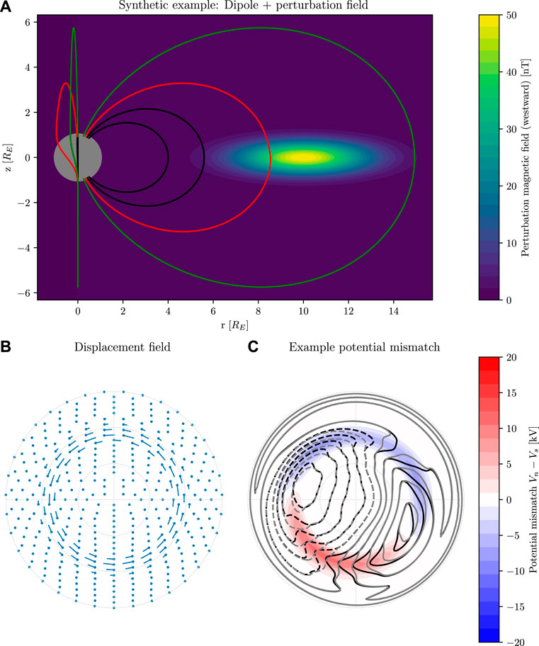
FIGURE 1. Conceptual illustration of the displacement field and its effect on ionospheric convection: (A) Magnetic field lines of a dipole magnetic field perturbed by a westward magnetic field indicated in color (a 2D Gaussian with peak value of 50 nT). The magnetic field lines are traced from − 60°, − 65° (black), − 70° (red), and − 75° (green) to the northern hemisphere. The dipole has a reference magnetic field (Fraser-Smith, 1987; Laundal and Richmond, 2017) of 28,000 nT. (B) The corresponding displacement field. The dots show footpoints in the southern hemisphere and the pins point to their conjugate point in the northern hemisphere, in a coordinate system where dipole magnetic field lines map to the same locations. In this, and in all subsequent polar plots, the view is down at the magnetic pole in the northern hemisphere, and through the Earth for the southern hemisphere, with noon on top and midnight at the bottom. The plots cover 60-90° latitude, with dashed circles every 10°. (C) An ionospheric convection electric potential in the southern hemisphere (grey) and the corresponding potential in the northern hemisphere (black) under the assumption that the potential maps along magnetic field lines between hemispheres. The color in the background show apparent potential misfit at coordinates that are connected by dipole magnetic field lines. The color scale used here is also used in subsequent figures.

Figure 1 is an example of how the displacement field can be calculated using field line tracing with perfect knowledge about the magnetic field surrounding the Earth, and how it influences the convection electric potential assuming ideal MHD. In the next section, we present a technique to estimate the displacement field δ(r) given perfect knowledge about the electric potential in the two hemispheres, Φ_N and Φ_S. We apply this to the idealized example in Figure 1 as an example. In Section 3 we present displacement fields implied by the Weimer (2005a),Weimer (2005b) empirical model of ionospheric convection given certain assumptions. We discuss results, limitations, and future prospects in Section 4.

2 Estimating the displacement field from convection maps

The relationship between the potentials in the two hemispheres and the footpoint displacement field δ gives that:

${\mathrm{\Phi }}_N\left(\mathbf{r}\right)={\mathrm{\Phi }}_S\left(\mathbf{r}+\mathit{\delta }\left(\mathit{r}\right)\right)\approx {\mathrm{\Phi }}_S\left(\mathbf{r}\right)-{\mathbf{E}}_S\left(\mathbf{r}\right)\cdot \mathit{\delta }\left(\mathit{r}\right),(2)$

where we used a first order Taylor expansion about r, and that E_S = −∇Φ_S. Rearranging the terms, we find a relationship between δ and the potential mismatch ΔΦ = Φ_N(r) − Φ_S(r):

${\mathbf{E}}_S\left(\mathbf{r}\right)\cdot \mathit{\delta }\left(\mathit{r}\right)=-\mathrm{\Delta }\mathrm{\Phi }.(3)$

Our aim is to find δ(r) given Φ_N and Φ_S. To accomplish this, Eq. 3 is not sufficient, and we need additional constraints. The following discussion is an effort to include such constraints using knowledge about the magnetosphere-ionosphere system.

The displacement field δ describes how a flux tube originating at (ϕ, −λ) in the Southern hemisphere, that nominally maps to (ϕ, λ) in the Northern hemisphere, now maps to a different location. ϕ and λ are here treated as longitude and latitude in modified Apex (MA) coordinates (Richmond, 1995). We use a MA reference radius R = R_E + 110 km, where R_E is the radius of the Earth. MA coordinates are defined such that ϕ and λ are constant along the magnetic field lines of a model magnetic field—usually the International Geomagnetic Reference Field (Alken et al., 2021), but in this paper a centered dipole. Assuming that the magnetospheric plasma and magnetic fields are frozen-in, the displacement δ is a result of past differences in convection in the two hemispheres. The simplest possible differential convection field that can produce the displacement is u = δ/ΔT, a constant velocity that is present for a time interval ΔT. If we also assume that the magnetic field changes slowly, Faraday’s law implies that u, and hence also δ relate to a potential field −∇α:

$\mathit{\delta }=\frac{-\nabla \alpha \times \mathbf{B}}{B^2}.(4)$

Now we represent α in terms of a set of basis functions. We use surface spherical cap harmonics (Haines, 1985; Fiori, 2020; Torta, 2020):

$\alpha =\sum _k^{25}\sum _m^{\text{max}\left(k,3\right)}{P}_{n_k\left(m\right)}^m\left(\sin \lambda \right)\left[g_k^m\cos \left(m\varphi \right)+h_k^m\sin \left(m\varphi \right)\right],(5)$

where $P_{n_k(m)}^m(\sin \lambda )$ are the Legendre functions of non-integer n_k(m) and integer m. Spherical cap harmonics map the global spherical harmonics to a spherical cap with a polar angle θ₀. We use θ₀ = 30°, which means that we do not consider displacements equatorward of 60°. The use of spherical cap harmonics has the advantage that certain boundary conditions can be applied in a straightforward way: We only use terms where k − m are even, which ensures that ∂P/∂λ = 0 for all k, m. α will therefore have zero gradient perpendicular to the equatorward boundary, and δ can only be in the meridional direction. We truncate the sum over spherical cap harmonics at k = 25, m = 3. This truncation level, which is more or less in line with previous models of polar ionospheric electrodynamics (e.g., Weimer, 2013), is presumably not a limiting factor for the spatial resolution of our solution compared to other effects discussed below.

With the spherical cap harmonic representation for α, Eq. 5, we have discretized Eq. 3, so that δ can be represented with 87 coefficients $g_k^m$ and $h_k^m$. To use this representation, we must evaluate the gradients of α and Φ, which are perpendicular to B since α and Φ are magnetic field-aligned. In MA coordinates, the gradients of α and Φ have only two non-zero components. We express E and δ in terms of MA basis vectors: $\mathbf{E}=E_{d_1}{\mathbf{d}}_1+E_{d_2}{\mathbf{d}}_2$ and $\mathit{\delta }={\delta }_{e_1}{\mathbf{e}}_1+{\delta }_{e_2}{\mathbf{e}}_2$. Equations 4.8, 4.9, 4.18, and 4.19 of Richmond (1995) give that:

$E_{S,d_1}=\frac{-1}{R\cos \lambda }\frac{\partial {\mathrm{\Phi }}_S}{\partial \varphi }(6)$

$E_{S,d_2}=\frac{1}{R\sin I}\frac{\partial {\mathrm{\Phi }}_S}{\partial \lambda }(7)$

${\delta }_{e_1}=\frac{1}{B_{e_3}R\sin I}\frac{\partial \alpha }{\partial \lambda }(8)$

${\delta }_{e_2}=\frac{1}{B_{e_3}R\cos \lambda }\frac{\partial \alpha }{\partial \varphi }(9)$

where

$\sin I=2\sin \lambda {\left(4-3{\cos }^2\lambda \right)}^{-1/2}.(10)$

$B_{e_3}={\mathbf{d}}_3\cdot \mathbf{B}$, where d₃ is a magnetic field-aligned basis vector in modified apex coordinates. For a dipole field $B_{e_3}=B_0{(4-3{\cos }^2\lambda )}^{1/2}$, the magnetic field strength at r = R. $B_{e_3}$ is constant along magnetic field lines. Here B₀ is ${(R_E/R)}^3$ times the reference magnetic field described by, e.g., Fraser-Smith (1987); Laundal and Richmond (2017). We use B₀ = 28, 000 nT.

Since d_i ⋅e_j = δ_ij, the dot product on the left hand side of Eq. (3) now gives:

$\frac{1}{B_0{R}^2\sin \left(2\lambda \right)}\left[\frac{\partial {\mathrm{\Phi }}_S}{\partial \varphi }\frac{\partial \alpha }{\partial \lambda }-\frac{\partial {\mathrm{\Phi }}_S}{\partial \lambda }\frac{\partial \alpha }{\partial \varphi }\right]=\mathrm{\Delta }\mathrm{\Phi }.(11)$

where we used the expressions for $B_{e_3}$ and sin I. Eq. 11 can now be used to construct a set of linear equations that relate the spherical harmonic coefficients which define α to the electric potential in the two hemispheres.

2.1 Choosing the right reference frame

Eq. 3 involves the electric field, which is a frame-dependent quantity. As discussed by Newell et al. (2004), ionospheric convection electric fields are normally given in an Earth-fixed reference frame, which does not include the rotational motion of the Earth. The arguments above build on the premise that E + v ×B = 0, which is a special case of the Generalized Ohm’s law/electron momentum equation where all terms except the Lorentz force are zero. Since acceleration terms must also be zero, we believe that it is appropriate to transform E_S to an inertial frame by including a co-rotation electric field.

For a dipole field, the co-rotation can be expressed as

${\mathbf{v}}_c=\omega R\cos \lambda {\mathbf{e}}_1,(12)$

where ω ≈ 2π/(24 h) is the rotation rate of the Earth. ωR cos λ is constant along magnetic field lines, and the variation in v_c is contained in e₁, which is an eastward unit vector at radius R for a dipole magnetic field. This motion corresponds to a co-rotation potential via Equation (8):

$\omega R\cos \lambda =\frac{1}{2B_{0}R\sin \lambda }\frac{\partial {\mathrm{\Phi }}_c}{\partial \lambda },(13)$

where we replaced $B_{e_3}$ with the dipole magnetic field strength at radius R, described above. Integrating this equation gives the co-rotation electric potential

${\mathrm{\Phi }}_c=\omega B_0{R}^2{\cos }^2\lambda +\mathrm{c}\mathrm{o}\mathrm{n}\mathrm{s}\mathrm{t}\mathrm{a}\mathrm{n}\mathrm{t}.(14)$

Since Φ_c is equal on opposite ends of unperturbed magnetic field lines, it does not contribute to ΔΦ in Eq. 3, but it does contribute to E_S. If we did not include co-rotation, Eq. 3 would not constrain δ in regions equatorward of the so-called Heppner-Maynard boundary (HMB) (Heppner and Maynard, 1987). Including co-rotation means that Eq. 3 helps to constrain δ in the direction perpendicular to e₁ × B also equatorward of the HMB.

2.2 Inversion

If Φ_N and Φ_S (now assumed to include Φ_C) are given on a set of N points, we have N equations for as many unknowns as there are spherical harmonic coefficients, L (in our case 87). This set of equations can in principle be solved by inversion. The task is essentially to find the set of coefficients $g_k^m$ and $h_k^m$ that describes a displacement field δ(r) which explains the observed potential mismatch ΔΦ. In matrix form, we write the set of equations as

$G\mathbf{m}=\mathbf{d},(15)$

where G is an N × L matrix, whose elements are given by Eq. 11 when (5) is used to represent α. m is an L-element vector composed of the spherical harmonic coefficients, and d is an N-element vector with the values of ΔΦ, the right-hand side of Eq. 11.

There are two major complicating factors in solving this set of equations for m: First of all, the arguments presented above only hold for closed magnetic field lines—field lines that connect the two hemispheres. A large region surrounding the magnetic poles do not connect to the opposite hemisphere but instead connect out in the solar wind. In these regions of open magnetic flux (the polar caps), we expect to see mismatches in the potentials (Crooker and Rich, 1993; Reistad et al., 2019, 2021) that are unrelated to magnetic field line displacements. In regions that map to reconnection, we also expect there to be magnetic field-aligned potential differences between hemispheres (Siscoe et al., 2001). Thus, there is a region near the poles where Eq. 3 should not be applied. Because of this we do not use data points poleward of ±78°.

Since the polar caps vary in size (e.g., Milan et al., 2003; Laundal et al., 2010), such a hard limit is problematic. We therefore use an inversion scheme that allows for outliers, since there may well be points equatorward of 78° which should be allowed to have large potential misfits. This is accomplished through iteratively re-weighted least squares, with zeroth-order Tikhonov regularization. The first step in this procedure is to calculate an initial model vector m₀, which represents the regularized least-squares solution:

${\mathbf{m}}_0={\left(G^{\top }G+\kappa I\right)}^{-1}{G}^{\top }\mathbf{d},(16)$

where κ is a regularization parameter and I is the L × L identity matrix. Next, a set of weights is calculated, as

$w_i=1/\mathrm{m}\mathrm{a}\mathrm{x}\left(ϵ,|d_{m,i}-d_i|\right),(17)$

where the index i gives the element in d, and d_m,i is the i’th element of the model prediction vector Gm₀. ϵ is a limit that prevents the weights from becoming extremely large. We use ϵ = 1 V, a low number considering that the potential mismatch is $\sim 1$ kV. After finding these weights, a second set of model parameters is calculated by calculating the weighted least-squares solution

${\mathbf{m}}_1={\left(G^{\top }\mathrm{diag}\left(\mathbf{w}\right)G+\kappa I\right)}^{-1}{G}^{\top }\mathrm{diag}\left(\mathbf{w}\right)\mathbf{d}.(18)$

New weights and new model vectors are calculated until the model vector converges.

In this way, the influence of outliers is greatly reduced. In other words, model vectors that give large areas with small potential mismatch are prioritized over model vectors that accommodate a few small regions with large misfit. Except for the regularization term, the procedure outlined above effectively minimizes the L1 norm of the model data misfit Gm − d (Aster et al., 2019).

The regularization parameter κ is needed because of a second major complication: Eq. 3 only constrains δ in the direction of E_S, and it only constrains δ where E_S is nonzero. In such regions, δ is only constrained by the property that it can be written in terms of a potential (Eq. 4) and by the boundary condition that we apply. The magnetic field line footpoints may be displaced along equipotentials, ending up on the same electric potential and observations of ΔΦ give no information about such displacements. We have no good fix for this problem, except to apply a conservative regularization scheme in the inversion to avoid artifacts, and to focus our analysis on regions that are well justified by coinciding electric fields.

2.3 Horizontal displacement field

The above procedure gives a set of model parameters m, which are coefficients in the spherical cap harmonic representation of α, Eq. 5. This, in turn, relates to modified apex components of the displacement field δ via Equations 8, 9. We have that

$\mathit{\delta }={\delta }_{e_1}{\mathbf{e}}_1+{\delta }_{e_2}{\mathbf{e}}_2,(19)$

where e₁ and e₂ are modified apex base vectors. In a dipole field at r = R, which we use throughout this paper, e₁ is equal to the eastward unit vector in SM coordinates $\widehat{\mathbf{e}}$. e₂ is also a unit vector but it has both horizontal and vertical components:

${\mathbf{e}}_2=\frac{-1}{\sqrt{4-3{\cos }^2\left(\lambda \right)}}\left(2\sin \lambda \widehat{\mathbf{n}}+\cos \lambda \widehat{\mathbf{r}}\right)(20)$

where $\widehat{\mathbf{n}}$ and $\widehat{\mathbf{r}}$ are unit vectors in the northward and radial directions in SM coordinates. In plots below, we show the horizontal SM components of δ. They can be written as

${\mathit{\delta }}_h={\delta }_{e_1}\widehat{\mathbf{e}}-\sin I_m{\delta }_{e_2}\widehat{\mathbf{n}}.(21)$

We note that in our implementation, we calculate the displaced coordinates at r + δ_h instead of mapping from r + δ to radius R. This simplification leads to an error which is very small since the magnetic field lines are close to vertical, and since δ is always relatively small.

2.4 A synthetic test

Figure 2 shows the result of the technique described above applied to the synthetic example from Figure 1. In this case, the main field is a dipole, and there are no open field lines so we include ΔΦs at high latitudes in the inversion. Apart from that, we use the regularization scheme described above. Figure 2 shows the synthetic (true) displacement field in blue (same as in Figure 1B) and the estimated δ in orange. The estimates are based on the potentials shown in Figure 2B. Figure 2C shows the same, except that the northern hemisphere potential (black) has been “corrected” by shifting every point by a distance − δ_h. We see that our δ removes most of the potential mismatch but not all.

FIGURE 2

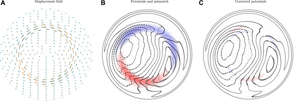
FIGURE 2. (A) The displacement field from Figure 1B, together with displacement field estimated using the technique described in Section 2 (orange pins). (B) The apparent potential mismatch that the displacement field is based on (a copy of Figure 1C), (C) The remaining potential mismatch when the estimated displacement field is taken into account in the comparison between hemispheres. The red-white-blue color scale is the same as in Figure 1.

In order to interpret the displacement fields that we derive in the next section, where we use statistical convection patterns from the two hemispheres, it is useful to compare the true displacement (blue) to the estimated displacement (orange) in Figure 2A. We see that they generally agree, but that there are notable deviations. For example, there are regions where δ is too small. This is likely due to the damping that we apply in order to avoid creating artifacts. Decreasing the damping parameter reduces the potential mismatch in Figure 2C, but the estimated displacement field deviates more from the truth. Increasing the damping parameter leads to larger potential mismatches and smaller displacement fields, but with less artificial structures. We use the same damping parameter in the real (next section) and synthetic (this section) cases.

3 The displacement field implied by the Weimer 2005 convection model

The main message of the previous section is that knowledge about the electric potentials in the two hemispheres gives information about the displacement field δ through Eq. (3). It is clear from the equation that δ is not fully determined: It gives no knowledge about δ in the direction perpendicular to the electric field, or in regions where the electric field is zero. The rest of Section 2 is basically an effort to maximize the utility of this equation by taking into account expected properties of δ: It can be derived from a scalar potential α that is magnetic field-aligned, and it is relatively smooth. The synthetic test shows that the technique still has limitations, and one should be careful in interpreting the results, especially displacements along equipotentials.

Nevertheless, in this section we apply the technique described above to convection patterns from the statistical model by Weimer (2005a),Weimer (2005b), which is based on measurements from the Dynamics Explorer 2 satellite. The statistical model outputs convection maps as a function of solar wind speed and density, interplanetary magnetic field, and dipole tilt angle. The IMF B_y component and the dipole tilt angle ψ are expected to influence inter-hemispheric asymmetries in both convection and magnetic field line footpoints. In fact, Weimer mixes observations from the two hemispheres by assuming that the potential in the south is the same as the potential in the north for opposite signs of B_y and ψ:

$\mathrm{\Phi }\left(\lambda ,B_y,\psi ,\dots \right)=\mathrm{\Phi }\left(-\lambda ,-B_y,-\psi ,\dots \right).(22)$

We have chosen convection maps for solar wind velocity 400 km/s, density 5 cm⁻³, and $\sqrt{B_y^2+B_z^2}=5$ nT. We investigate three different combinations of IMF clock angle, arctan2(B_y, B_z); −225°, −180°, and 135°; and three different combinations of dipole tilt angle: ψ = −20°, 0°, and 20°. This gives a total of nine combinations. We estimate the interhemispheric displacement field implied by these convection patterns, given the assumptions and caveats discussed in the previous section.

The convection potentials from the northern (black) and southern (grey) hemispheres for the nine different combinations are shown in Figure 3. Co-rotation has been added using the equations of Section 2.1. Because of Equation 22, the panels should be symmetric about the center, and the potentials in the center are exactly equal. Deviations from symmetry must be due to numerical effects related to the interpolation of the Weimer (2005a,b) potentials from the original grid to our evaluation points and in later figures also numerical effects related to the inversion.

FIGURE 3

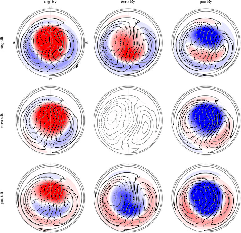
FIGURE 3. Nine different Weimer (2005a),Weimer (2005b) electric potentials from the southern (grey) and northern (black) hemispheres. The color shows the potential mismatch at matching coordinates, using the color scale from Figure 1. For all panels the solar wind velocity is 400 km/s, density 5 cm⁻³, and $\sqrt{B_y^2+B_z^2}=5$ nT. The three columns correspond to three different combinations of IMF clock angle, arctan2 (B_y, B_z); −225°, − 180°, and 135°. The three rows correspond to three different combinations of dipole tilt angle: ψ = −20°, 0°, and 20°.

Figure 3 shows large potential mismatches (the color scale is the same as in Figure 1), especially near the pole. Figure 4 shows the same convection potentials after shifting Φ_N by an amount δ, where the displacement field δ is estimated as explained in the previous section. We see that the potential mismatches are significantly reduced, except for near the poles. This means that the displacement field that we have derived explains much of the mismatch on closed magnetic field lines.

FIGURE 4

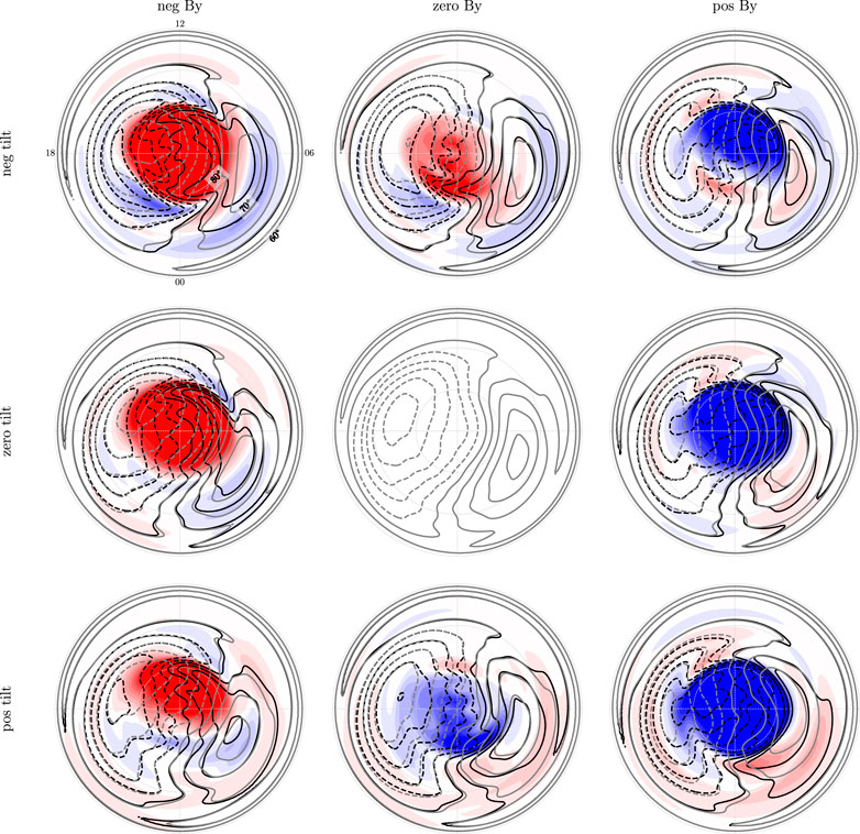
FIGURE 4. Weimer (2005a),Weimer (2005b) electric potentials in the same format as in Figure 3, but with the Northern hemisphere potentials shifted using our estimated displacement field. The red-white-blue color scale is the same as in Figure 1.

The actual displacement field (δ_h) is shown in Figure 5. The pins show where magnetic field lines in the northern hemisphere that nominally map to the dot are shifted. We notice the following: 1) The displacement fields are non-uniform, which means that single point observations of field-line footpoint displacement (Østgaard et al., 2004; Østgaard et al., 2011; Ohma et al., 2018) are not enough to describe how the two hemispheres are connected. This point was also well illustrated by Ganushkina et al. (2013), who investigated latitudinal and longitudinal displacements in footpoint location using the Tsyganenko (2002) model. 2) The displacement is typically strongest in the midnight sector, and 3) this displacement appears to depend more strongly on the dipole tilt angle than on the sign of the IMF B_y. It is also interesting to note that the displacement field changes sign along the midnight meridian in all maps. We also see features in the displacement field which are almost certainly artifacts: The westward pins at $\sim 65°$ post-noon in the top row (eastward in the bottom row) are more or less along equipotential contours. Including them in (Eq. 3) would not significantly increase or decrease ΔΦ, which means that their existence (or non-existence) is not substantiated by the observed potentials.

FIGURE 5

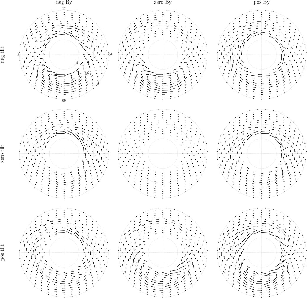
FIGURE 5. The displacement fields estimated from the potentials in Figure 3.

The strong dependence on dipole tilt angle is surprising. Observations of substorm onsets indicate that the effect of dipole tilt angle on magnetic field line footpoint displacement is weak (Elhawary et al., 2022). It is also surprising that the dipole tilt effect is in the same direction across the nightside. When the dipole axis is tilted, the tail is expected to “warp” tailward of the inner dipolar magnetic field lines (Fairfield, 1979; Liou and Newell, 2010). The warping of the tail would imply an additional B_y component with opposite signs at dawn and dusk (Petrukovich, 2011).

The B_y dependence seen in the displacement field is more expected: If we ignore the tilt effect, by looking at middle row, we see that positive B_y tends to give a displacement field that points from dawn to dusk, consistent with a B_y component induced in the magnetosphere as explained by Tenfjord et al. (2015), and observed by Wing et al. (1995); Tenfjord et al. (2017); Tsyganenko (2002). Negative B_y gives displacement fields in the opposite direction. These fields appear to maximize on the noon-midnight meridian, which is also in line with expectations. The reversal at higher latitudes is however not expected from modeling and observations. One possible explanation is that field lines poleward of the reversal are on average open.

It is also interesting to note that the largest displacements are seen when B_y and tilt have the same sign. This was also observed by Petrukovich (2009) whose observations of B_y in the tail did not behave as one would expect from the warping effect, but instead showed that B_y correlates with dipole tilt angle at midnight and pre-midnight, and no effect post-midnight. This is more in line with the uniform displacement field seen on the nightside Figure 5. The magnitude of the dipole tilt angle effect seen in Figure 5, when compared to the B_y effect, is still surprising. In sum, comparisons with previous studies give good reason to be skeptical to the results presented in Figure 5. We elaborate on this skepticism in the next section.

4 Discussion

In this paper we have introduced the concept of a displacement field, a 2D vector field on a spherical shell that describes how magnetic field line footpoints in the northern hemisphere are displaced relative to their southern counterpart due to perturbations in the magnetic field of the magnetosphere. The concept of a non-uniform displacement vector field goes beyond previous studies that have studied the displacement at single points (Frank and Sigwarth, 2003; Østgaard et al., 2004; Østgaard et al., 2005; Ohma et al., 2018). We have argued that the displacement field must have the same mathematical properties as plasma convection in the F-region, where ideal MHD is assumed to be valid. It can be related to a scalar field (called α in this paper). We showed how the displacement field is related to the ionospheric convection in the two hemispheres in regions of closed magnetic field lines, and used this to estimate displacement fields implied by the Weimer (2005a),Weimer (2005b) empirical model of ionospheric convection.

We see a clear reduction in potential mismatch in the Weimer model with our derived displacement field (Figure 4 compared to Figure 3). This means that the displacement field and Weimer model are consistent to the extent of the remaining mismatch; but we should still be careful in reading too much into the estimated displacement fields. We have discussed some reasons for this above: The lack of information that we get from Eq. 3 where E_S ⋅δ = 0, and the challenge in determining which regions to consider as covered by closed magnetic field lines. A third reason to be skeptical about the result is that the Weimer (2005a),Weimer (2005b) model was not designed to be consistent with a realistic displacement field. We expect that the uncertainty in electric potential values, which we use in our calculations, may be relatively large. The reason for this is that the model is constrained by measurements of the derivative of the potential and not by the potential itself. For example, regions in the Weimer model where the potential variations are small could lead to large and unrealistic displacements with our method. These regions would be based on measurements of weak plasma velocity, and it should not be expected that the coinciding potential contours are precisely determined. Nevertheless, we used the Weimer (2005a),Weimer (2005b) model in this paper because it is very well established, and we are not aware of any other empirical model that would be better suited for our purposes. The main purpose of estimating the displacement field in this way is to show that it is possible to link the two hemispheres using the assumption of ideal MHD, and that differences in convection electric potentials are related to the integrated effect of magnetic perturbations on the footpoints of closed magnetic field lines.

The displacement field shows how magnetic field line footpoints in the northern hemisphere are displaced relative to the expected position when tracing along a magnetic field model from the southern hemisphere. The Altitude-Adjusted Corrected Geomagnetic Coordinate system (Shepherd, 2014) and the Apex coordinate systems (VanZandt et al., 1972; Richmond, 1995) are constructed so that corresponding coordinates in the two hemispheres belong to the same model magnetic field line. We have used a dipole model, but one could also use more realistic models like the full International Geomagnetic Reference Field (Alken et al., 2021). Papitashvili et al. (1997) presented a coordinate system based on Tsyganenko (1989)’s model of the magnetospheric magnetic field. With such a model, if it is accurate, the ionospheric convection electric potential should be equal on matching coordinates (again assuming ideal MHD). Using this property with a modern magnetospheric model may be the most feasible way to construct an empirical model of ionospheric convection that by design is consistent in the two hemispheres.

A series of papers have explored the coupled hemispheres from an electric circuit perspective: Benkevich et al. (2000); Lyatskaya et al. (2014) suggested that incident magnetic field-aligned currents in one hemisphere can be redistributed in the ionosphere in both hemispheres via horizontal and interhemispheric field-aligned currents. The interhemispheric currents would primarily be located at the sunlight terminator where, from a circuit point of view, it would be easier to close currents in the opposite sunlit hemisphere. Observational tests of these ideas have not found such inter-hemispheric currents to exist (Østgaard et al., 2016). The models predicting inter-hemispheric currents did not take into account any displacement between magnetic field line footpoints. With the approach in the present paper, steady-state electric currents and the displacement field δ can be related if we also know the ionospheric conductance, by use of the ionospheric Ohm’s law. Whether or not the implied currents in the two hemispheres are connected to each other, or connect to other currents along the way in the magnetosphere, is not possible to tell by considering ionospheric observations alone.

Since we lack continuous observations of conjugate auroras, and since convection electric potential estimates are inaccurate, the best way to study the displacement field is probably with simulations. Ohma et al. (2021) showed that the displacement field reduces in step with nightside reconnection. However, they did not link the displacement to ionospheric convection. One reason why this may not be straightforward is that the ionospheric electric field in MHD codes is calculated independently in the two hemispheres, and there is therefore no guarantee that the potential matches on opposite ends of closed magnetic field lines. If it does not match, it means that there is a potential drop along magnetic field lines between hemispheres, in violation of the fundamental assumption of such models: That ideal MHD is valid. The displacement field and its relation to ionospheric electric potentials could be used to remove this possible inconsistency, by requiring that Φ_N(r) = Φ_S (r + δ) on closed field lines. δ can be calculated by magnetic field line tracing, or by keeping track of the differences in ionospheric convection in the two hemispheres over time.

On the observational side, the most direct way of estimating displacement fields is to match features in the aurora. However, this has so far been done only on a point by point basis, when two satellites have happened to observe the two hemispheres simultaneously. A dedicated satellite mission to observe the aurora in both hemispheres (Branduardi-Raymont et al., 2021) would undoubtedly reveal the displacement field in much more detail, and greatly increase our understanding of geospace as a coupled two-hemisphere system.

Data availability statement

Publicly available datasets were analyzed in this study. This data can be found here: https://github.com/klaundal/displacement_field.

Author contributions

KL had the idea for the study, wrote the code and manuscript. MM made critical contributions to the inversion technique. AO helped with field line tracing and testing of the technique. JR and SH helped develop the idea, and supported the work throughout the process. All authors read and commented on the manuscript.

Funding

The work was funded by the Trond Mohn Foundation, and by the Research Council of Norway under contracts 223252/F50 and 300844/F50.

Weimer 2005 convection model output was provided by the Community Coordinated Modeling Center (CCMC) at Goddard Space Flight Center through their publicly available simulation services (https://ccmc.gsfc.nasa.gov). We are grateful to DW, Virginia Tech, for developing the Weimer 2005 model and for making it available via CCMC.

Conflict of interest

The authors declare that the research was conducted in the absence of any commercial or financial relationships that could be construed as a potential conflict of interest.

Publisher’s note

All claims expressed in this article are solely those of the authors and do not necessarily represent those of their affiliated organizations, or those of the publisher, the editors and the reviewers. Any product that may be evaluated in this article, or claim that may be made by its manufacturer, is not guaranteed or endorsed by the publisher.

References

Alken, P., Thébault, E., Beggan, C. D., Amit, H., Aubert, J., Baerenzung, J., et al. (2021). International geomagnetic reference field: The thirteenth generation. Earth Planets Space 73, 49. doi:10.1186/s40623-020-01288-x

CrossRef Full Text | Google Scholar

Aster, R. C., Borchers, B., and Thurber, C. H. (2019). “Chapter two - linear regression,” in Parameter estimation and inverse problems. Editors R. C. Aster, B. Borchers, and C. H. Thurber. 3rd edition (Netherland: Elsevier), 25–53. doi:10.1016/B978-0-12-804651-7.00007-9

CrossRef Full Text | Google Scholar

Benkevich, L., Lyatsky, W., and Cogger, L. L. (2000). Field-aligned currents between conjugate hemispheres. J. Geophys. Res. 105, 27727–27737. doi:10.1029/2000ja900095

CrossRef Full Text | Google Scholar

Branduardi-Raymont, G., Berthomier, M., Bogdanova, Y. V., Carter, J. A., Collier, M., Dimmock, A., et al. (2021). Exploring solar-terrestrial interactions via multiple imaging observers. Exp. Astron. (Dordr). doi:10.1007/s10686-021-09784-y

CrossRef Full Text | Google Scholar

Crooker, N. U., and Rich, F. J. (1993). Lobe cell convection as a summer phenomenon. J. Geophys. Res. 98, 13403–13407. doi:10.1029/93JA01037

CrossRef Full Text | Google Scholar

Elhawary, R., Laundal, K. M., Reistad, J. P., and Hatch, S. M. (2022). Possible ionospheric influence on substorm onset location. Geophys. Res. Lett. 49, e2021GL096691. doi:10.1029/2021GL096691

CrossRef Full Text | Google Scholar

Fairfield, D. H. (1979). On the average configuraton of the geomagnetic tail. J. Geophys. Res. 84, 1950–1958. doi:10.1029/ja084ia05p01950

CrossRef Full Text | Google Scholar

Fiori, R. A. D. (2020). “Spherical cap harmonic analysis techniques for mapping high-latitude ionospheric plasma flow—application to the swarm satellite mission,” in Ionospheric multi-spacecraft analysis tools. ISSI scientific report series. Editors M. Dunlop, and H. Lühr (Cham: Springer), 17. doi:10.1007/978-3-030-26732-2_9

CrossRef Full Text | Google Scholar

Förster, M., and Haaland, S. (2015). Interhemispheric differences in ionospheric convection: Cluster EDI observations revisited. J. Geophys. Res. Space Phys. 120, 5805–5823. doi:10.1002/2014JA020774

CrossRef Full Text | Google Scholar

Frank, L. A., and Sigwarth, J. B. (2003). Simultaneous images of the northern and southern auroras from the Polar spacecraft: An auroral substorm. J. Geophys. Res. 108, 8015. doi:10.1029/2002JA009356

CrossRef Full Text | Google Scholar

Fraser-Smith, A. C. (1987). Centered and eccentric geomagnetic dipoles and their poles, 1600-1985. Rev. Geophys. 25, 1–16. doi:10.1029/rg025i001p00001

CrossRef Full Text | Google Scholar

Ganushkina, N. Y., Kubyshkina, M. V., Partamies, N., and Tanskanen, E. (2013). Interhemispheric magnetic conjugacy. J. Geophys. Res. Space Phys. 118, 1049–1061. doi:10.1002/jgra.50137

CrossRef Full Text | Google Scholar

Grocott, A., Milan, S. E., and Yeoman, T. K. (2008). Interplanetary magnetic field control of fast azimuthal flows in the nightside high-latitude ionosphere. Geophys. Res. Lett. 35, L08102. doi:10.1029/2008GL033545

CrossRef Full Text | Google Scholar

Grocott, A., Yeoman, T. K., Milan, S. E., and Cowley, S. W. H. (2005). Interhemispheric observations of the ionospheric signature of tail reconnection during IMF-northward non-substorm intervals. Ann. Geophys. 23, 1763–1770. doi:10.5194/angeo-23-1763-2005

CrossRef Full Text | Google Scholar

Haines, G. V. (1985). Spherical cap harmonic analysis. J. Geophys. Res. 90, 2583–2591. doi:10.1029/JB090iB03p02583

CrossRef Full Text | Google Scholar

Heppner, J. P., and Maynard, N. C. (1987). Empirical high-latitude electric field models. J. Geophys. Res. 92, 4467–4489. doi:10.1029/JA092iA05p04467

CrossRef Full Text | Google Scholar

Hesse, M., Birn, J., and Hoffman, R. A. (1997). On the mapping of ionospheric convection into the magnetosphere. J. Geophys. Res. 102, 9543–9551. doi:10.1029/96JA03999

CrossRef Full Text | Google Scholar

Laundal, K. M., Finlay, C. C., Olsen, N., and Reistad, J. P. (2018). Solar wind and seasonal influence on ionospheric currents from Swarm and CHAMP measurements. J. Geophys. Res. Space Phys. 123, 4402–4429. doi:10.1029/2018JA025387

CrossRef Full Text | Google Scholar

Laundal, K. M., Østgaard, N., Snekvik, K., and Frey, H. U. (2010). Inter-hemispheric observations of emerging polar cap asymmetries. J. Geophys. Res. 115. doi:10.1029/2009JA015160

CrossRef Full Text | Google Scholar

Laundal, K. M., and Richmond, A. D. (2017). Magnetic coordinate systems. Space Sci. Rev. 206, 27–59. doi:10.1007/s11214-016-0275-y

CrossRef Full Text | Google Scholar

Liou, K., and Newell, P. T. (2010). On the azimuthal location of auroral breakup: Hemispheric asymmetry. Geophys. Res. Lett. 37. doi:10.1029/2010GL045537

CrossRef Full Text | Google Scholar

Longden, N., Chisham, G., Freeman, M. P., Abel, G. A., and Sotirelis, T. (2010). Estimating the location of the open-closed magnetic field line boundary from auroral images. Ann. Geophys. 28, 1659–1678. doi:10.5194/angeo-28-1659-2010

CrossRef Full Text | Google Scholar

Lyatskaya, S., Khazanov, G. V., and Zesta, E. (2014). Interhemispheric field-aligned currents: Simulation results. J. Geophys. Res. Space Phys. 119, 5600–5612. doi:10.1002/2013ja019558

CrossRef Full Text | Google Scholar

Milan, S. E., Lester, M., Cowley, S. W. H., Oksavik, K., Brittnacher, M., Greenwald, R. A., et al. (2003). Variations in the polar cap area during two substorm cycles. Ann. Geophys. 21, 1121–1140. doi:10.5194/angeo-21-1121-2003

CrossRef Full Text | Google Scholar

Newell, P. T., Ruohoniemi, J. M., and Meng, C.-I. (2004). Maps of precipitation by source region, binned by IMF, with inertial convection streamlines. J. Geophys. Res. 109, A10206. doi:10.1029/2004JA010499

CrossRef Full Text | Google Scholar

Ohma, A., Østgaard, N., Laundal, K. M., Reistad, J. P., Hatch, S. M., Tenfjord, P., et al. (2021). Evolution of IMF B_y induced asymmetries: The role of tail reconnection. J. Geophys. Res. Space Phys. 126, e2021ja029577. doi:10.1029/2021JA029577

CrossRef Full Text | Google Scholar

Ohma, A., Østgaard, N., Reistad, J. P., Tenfjord, P., Laundal, K. M., Snekvik, K., et al. (2018). Evolution of asymmetrically displaced footpoints during substorms. J. Geophys. Res. Space Phys. 123, 10,030–10,063. doi:10.1029/2018JA025869

CrossRef Full Text | Google Scholar

Østgaard, N., Humberset, B. K., and Laundal, K. M. (2011). Evolution of auroral asymmetries in the conjugate hemispheres during two substorms. Geophys. Res. Lett. 38. doi:10.1029/2010GL046057

CrossRef Full Text | Google Scholar

Østgaard, N., Mende, S. B., Frey, H. U., Immel, T. J., Frank, L. A., Sigwarth, J. B., et al. (2004). Interplanetary magnetic field control of the location of substorm onset and auroral features in the conjugate hemispheres. J. Geophys. Res. 109, A07204. doi:10.1029/2003JA010370

CrossRef Full Text | Google Scholar

Østgaard, N., Reistad, J. P., Tenfjord, P., Laundal, K. M., Rexer, T., Haaland, S. E., et al. (2018). The asymmetric geospace as displayed during the geomagnetic storm on 17 August 2001. Ann. Geophys. 36, 1577–1596. doi:10.5194/angeo-36-1577-2018

CrossRef Full Text | Google Scholar

Østgaard, N., Reistad, J. P., Tenfjord, P., Laundal, K. M., Snekvik, K., Milan, S., et al. (2016). “Mechanisms that produce auroral asymmetries in conjugate hemispheres,” in Auroral dynamics and Space weather, geophysical monograph 215 (New York: John Wiley & Sons), 133–144.

Google Scholar

Østgaard, N., Tsyganenko, N. A., Mende, S. B., Frey, H. U., Immel, T. J., Fillingim, M., et al. (2005). Observations and model predictions of substorm auroral asymmetries in the conjugate hemispheres. Geophys. Res. Lett. 32, L05111. doi:10.1029/2004GL022166

CrossRef Full Text | Google Scholar

Papitashvili, V. O., Papitashvili, N. E., and King, J. H. (1997). Magnetospheric geomagnetic coordinates for space physics data presentation and visualization. Adv. Space Res. 20, 1097–1100. doi:10.1016/s0273-1177(97)00565-6

CrossRef Full Text | Google Scholar

Petrukovich, A. A. (2009). Dipole tilt effects in plasma sheet b_y : Statistical model and extreme values. Ann. Geophys. 27, 1343–1352. doi:10.5194/angeo-27-1343-2009

CrossRef Full Text | Google Scholar

Petrukovich, A. A. (2011). Origins of plasma sheet b_y. J. Geophys. Res. 116. doi:10.1029/2010JA016386

CrossRef Full Text | Google Scholar

Pettigrew, E. D., Shepherd, S. G., and Ruohoniemi, J. M. (2010). Climatological patterns of high-latitude convection in the Northern and Southern hemispheres: Dipole tilt dependencies and interhemispheric comparisons. J. Geophys. Res. 115. doi:10.1029/2009JA014956

CrossRef Full Text | Google Scholar

Qian, L., Burns, A. G., Emery, B. A., Foster, B., Lu, G., Maute, A., et al. (2014). The NCAR TIE-GCM. Washington: American Geophysical Union, 73–83. chap. 7. doi:10.1002/9781118704417.ch7

CrossRef Full Text | Google Scholar

Reistad, J. P., Laundal, K. M., Østgaard, N., Ohma, A., Burrell, A. G., Hatch, S. M., et al. (2021). Quantifying the lobe reconnection rate during dominant IMF B_y periods and different dipole tilt orientations. JGR. Space Phys. 126, e2021JA029742. doi:10.1029/2021JA029742

CrossRef Full Text | Google Scholar

Reistad, J. P., Laundal, K. M., Østgaard, N., Ohma, A., Thomas, E., Haaland, S., et al. (2019). Separation and quantification of ionospheric convection sources: 1. A new technique. JGR. Space Phys. 124, 6343–6357. doi:10.1029/2019JA026634

CrossRef Full Text | Google Scholar

Reistad, J. P., Østgaard, N., Tenfjord, P., Laundal, K. M., Snekvik, K., Haaland, S., et al. (2016). Dynamic effects of restoring footpoint symmetry on closed magnetic field lines. J. Geophys. Res. Space Phys. 121, 3963–3977. doi:10.1002/2015JA022058

CrossRef Full Text | Google Scholar

Richmond, A. D. (1995). Ionospheric electrodynamics using magnetic apex coordinates. J. Geomagn. Geoelec. 47, 191–212. doi:10.5636/jgg.47.191

CrossRef Full Text | Google Scholar

Shepherd, S. G. (2014). Altitude-adjusted corrected geomagnetic coordinates: Definition and functional approximations. J. Geophys. Res. Space Phys. 119, 7501–7521. doi:10.1002/2014JA020264

CrossRef Full Text | Google Scholar

Siscoe, G. L., Erickson, G. M., Sonnerup, B. U. O., Maynard, N. C., Siebert, K. D., Weimer, D. R., et al. (2001). Global role of E_∥ in magnetopause reconnection: An explicit demonstration. J. Geophys. Res. 106, 13015–13022. doi:10.1029/2000JA000062

CrossRef Full Text | Google Scholar

Tenfjord, P., Østgaard, N., Snekvik, K., Laundal, K. M., Reistad, J. P., Haaland, S., et al. (2015). How the IMF by induces a by component in the closed magnetosphere and how it leads to asymmetric currents and convection patterns in the two hemispheres. J. Geophys. Res., 9368–9384. doi:10.1002/2015JA02157

CrossRef Full Text | Google Scholar

Tenfjord, P., Østgaard, N., Strangeway, R., Haaland, S., Snekvik, K., Laundal, K. M., et al. (2017). Magnetospheric response and reconfiguration times following IMF B_y reversals. J. Geophys. Res. Space Phys. 122, 417–431. doi:10.1002/2016JA023018

CrossRef Full Text | Google Scholar

Thomas, E. G., and Shepherd, S. G. (2018). Statistical patterns of ionospheric convection derived from mid-latitude, high-latitude, and polar superdarn hf radar observations. J. Geophys. Res. Space Phys. 123, 3196–3216. doi:10.1002/2018JA025280

CrossRef Full Text | Google Scholar

Torta, J. M. (2020). Modelling by spherical cap harmonic analysis: A literature review. Surv. Geophys. 41, 201–247. doi:10.1007/s10712-019-09576-2

CrossRef Full Text | Google Scholar

Tsyganenko, N. A. (1989). A magnetospheric magnetic field model with a warped tail current sheet 37, Planet. Space Sci. 37. 5–20.

CrossRef Full Text | Google Scholar

Tsyganenko, N. A. (2002). A model of the near magnetosphere with a dawn-dusk asymmetry 1. Mathematical structure. J. Geophys. Res. 107, SMP 12-1–SMP 12-15. doi:10.1029/2001JA000219

CrossRef Full Text | Google Scholar

VanZandt, T. E., Clark, W. L., and Warnock, J. W. (1972). Magnetic apex coordinates: A magnetic coordinate system for the ionospheric F2 layer. J. Geophys. Res. 77, 2406–2411. doi:10.1029/ja077i013p02406

CrossRef Full Text | Google Scholar

Weimer, D. (2001). Maps of ionospheric field-aligned currents as a function of the interplanetary magnetic field derived from Dynamics Explorer 2 data. J. Geophys. Res. 106, 12889–12902. doi:10.1029/2000ja000295

CrossRef Full Text | Google Scholar

Weimer, D. R. (2013). An empirical model of ground-level geomagnetic perturbations. Space weather. 11, 107–120. doi:10.1002/swe.20030

CrossRef Full Text | Google Scholar

Weimer, D. R. (2005a). Improved ionospheric electrodynamic models and application to calculating joule heating rates. J. Geophys. Res. 110, A05306. doi:10.1029/2004JA010884

CrossRef Full Text | Google Scholar

Weimer, D. R. (2005b). Predicting surface geomagnetic variations using ionospheric electrodynamic models. J. Geophys. Res. 110, A12307. doi:10.1029/2005JA011270

CrossRef Full Text | Google Scholar

Wing, S., Newell, P. T., Sibeck, D. G., and Baker, K. B. (1995). A large statistical study of the entry of interplanetary magnetic field y-component into the magnetosphere. Geophys. Res. Lett. 22, 2083–2086. doi:10.1029/95gl02261

CrossRef Full Text | Google Scholar