 Michael Madelaire
 Karl M. Laundal
 Jone P. Reistad
 Spencer M. Hatch
 Anders Ohma
- Birkeland Centre for Space Science, Bergen, Norway
Rapid changes in solar wind dynamic pressure can produce a transient geomagnetic response in the high latitude ionosphere. In this study we carry out a superposed epoch analysis of the geomagnetic response based on 2,058 events. The events are divided into 12 groups based on interplanetary magnetic field clock angle and dipole tilt and the magnetic perturbation field is modeled using spherical harmonics. We find that the high latitude transient current vortices associated with a sudden commencement are most clearly observed when the interplanetary magnetic field is northward during equinox and winter in the northern hemisphere. The high latitude geomagnetic response during northward interplanetary magnetic field is decomposed into a preliminary and main impulse. The preliminary impulse onset is 1–2 min prior to the onset of the low/mid latitude geomagnetic response and its rise time is 4–6 min. The main impulse onset is around 2 min after the low/mid latitude geomagnetic response and has a rise time of 6–11 min. When examining the change relative to pre-onset conditions a coherent transient geomagnetic response emerges for all IMF clock and dipole tilt angles. The current vortex associated with the main impulse on the dawnside appears at (9.3 ± 0.5 mlt, 64.8° ± 1.5° mlat) and moves westward with a velocity of 5 ± 1.4 km/s. The vortex on the duskside appears at (15.3 ± 0.9 mlt, 65.8° ± 2.5° mlat) and does not move significantly. In addition, the models were used to recreate the SMR index showing a significant mlt dependence on the magnetic perturbation above 40° mlat and below 10° mlat. The former is thought to be caused by high latitude ionospheric currents. The latter is potentially a combination of the event occurrence probability being skewed toward certain UT ranges for large dipole tilt angles and a UT dependence of the equatorial electrojet magnitude caused by the south atlantic magnetic anomaly.
1 Introduction
A (Storm) Sudden Commencement (SC) occurs when a rapid increase in solar wind dynamic pressure (Pd) impinges on our magnetosphere. These events are interesting as they allow us to observe a perturbation of the system and the subsequent transient response that unfolds in the following 10 s of minutes. In this study we focus on the geomagnetic response as observed from ground magnetometers and define SC as independent of whether or not it is followed by a geomagnetic storm as suggested by Curto et al. (2007).
SCs were initially thought to be associated with flux transfer events, but their connection to rapid changes in Pd was later shown in two case studies (Friis-Christensen et al., 1988; Glassmeier et al., 1989). In each study ground magnetometers were used to infer the ionospheric equivalent current which revealed transient current vortices.
A few years later Sibeck (1990), Kivelson and Southwood (1991) and Glassmeier and Heppner (1992) published theories on a mechanism that generates transient ionospheric current vortices. They all suggested that a shear flow close to the magnetopause or low-latitude boundary layer would give rise to Field Aligned Currents (FACs) that map to the ionosphere. However, they disagreed on the expected response. Sibeck (1990) and Kivelson and Southwood (1991) argue that the arrival of the solar wind pressure structure will launch a compression wave in the magnetosphere. This wave is faster than the solar wind in the magnetosheath and results in an expansion followed by a contraction of the magnetopause and thus two sets of twin vortices are created. Glassmeier and Heppner (1992) argues that a pressure pulse will create two sets of twin vortices while a single pressure increase/decrease will only result in a single set of twin vortices. Alternatively, it was suggested by Araki (1994), building on Tamao (1964), that the compression wave undergoes a mode conversion to a transverse mode inside the magnetosphere where gradients in Alfvenic speeds are large. Beside the theory of the underlying mechanism Araki (1994) presented a model of the expected response, Dsc, which was decomposed into two parts.
DL refers to a step-like increase in the horizontal magnetic field component at low/mid latitudes due to an increased magnetopause current. DP refers to the ionospheric response dominant at high latitudes and is itself composed of two parts.
The preliminary impulse PI and main impulse MI both refer to two sets of twin transient high latitude ionospheric current vortices generated during the SC (Araki, 1994). The PI is the first set of current vortices that are generated on the dayside i.e. one at pre-noon and another at post-noon. The electric current in the pre-noon vortex flows anti-clockwise while the current in the post-noon vortex is clockwise, i.e., similar to the NBZ current vortices generated during northward IMF due to lobe reconnection (Cowley and Lockwood, 1992). The MI is the second set of vortices, also generated at pre- and post-noon, however, the current flows opposite to that of the PI vortices, i.e., similar to that of the region 1/region 2 (R1/R2) current vortices (Cowley and Lockwood, 1992).
Our goal is to determine the influence of environmental parameters, such as Interplanetary Magnetic Field (IMF) clock angle and dipole tilt, on the development of the high latitude geomagnetic response to rapid increases in Pd. Due to the lack of data (events) in previous studies it has not been possible to carry out statistical studies on more than one environmental parameter without compromising the statistical integrity.
Many case studies of SCs have been conducted, e.g., Lam and Rodger (2001) tested the physical model presented by Araki (1994) against a single event. They found good correspondence between predictions and observations at high latitudes on the dayside while the predictions were less reliable at low latitudes and at night. Moretto et al. (2000) modeled the high latitude ionospheric response and resolved both growth and decay of current vortices, however, their propagation did not agree with Araki (1994), thus questioning the validity of the physical models with respect to real events. They noted that the shock normal was not parallel to the Sun-Earth line and might therefore result in an asymmetric geospace response which Araki (1994) did not take into account.
It is difficult to find instances where sensors are aligned optimally in the solar wind, magnetosheath, magnetosphere and on ground such that a full picture of the geospace response can be observed. Magnetohydrodynamic (MHD) simulations are therefore a very powerful tool as they provide a controlled environment where everything can be observed. Many studies have utilized MHD simulations in attempts to understand both the magnetospheric origin and the ionospheric response during rapid increases of Pd (Slinker et al., 1999; Keller et al., 2002; Fujita et al., 2003a,b, 2005; Ridley et al., 2006; Samsonov et al., 2010; Samsonov and Sibeck, 2013; Shi et al., 2014; Welling et al., 2021). These studies differ in several aspects. The MHD code used varies and in some cases the solar wind parameters uphold the Rankine-Hugoniot jump conditions and other times they do not. Some studies model common pressure changes while others model Carrington-like events. With these variabilities it is understandable that the resulting conclusions as to the magnetospheric origin also vary. Some studies agree with Araki (1994) that the magnetospheric vortices are generated inside the magnetosphere while others conclude that they are generated at the magnetopause. The studies conducted by Samsonov et al. (2010); Samsonov and Sibeck (2013) stand out as they do not agree with any of the preexisting theories. They suggest that the initial compression wave reflects on an inner boundary, probably the ionosphere, resulting in a sunward moving wave which by interacting with the anti-sunward flow creates a shear.
Russell et al. (1994a,b) and Russell and Ginskey (1995) present statistical studies of the geomagnetic response at low/mid latitudes during northward and southward IMF conditions. They found the geomagnetic response to be 18.4 nT/nPa1/2 during northward IMF while it is 13.8 nT/nPa1/2 (25% less) during southward IMF. Stauning and Troshichev (2008), Huang (2005) and Madelaire et al. (2022) carried out statistical studies of the transient high latitude response using the PCN index (World Data Center For Geomagnetism, Copenhagen, 2019), i.e., the Northern Polar Cap and refers to an index based on a single ground magnetometer station (Thule) close to the northern magnetic pole that attempts to quantify anti-sunward plasma convection in the polar cap. They found that the DPPI and DPMI corresponds to a negative and positive excursion in the PCN index, respectively. Madelaire et al. (2022) showed that the DPPI and DPMI peaked around 3 and 9 min after onset of the DL response. In addition, Stauning and Troshichev (2008) created maps of the equivalent ionospheric current using ground magnetometers showing the creation and decay of ionospheric current vortices, however, no environmental parameters were taken into account.
In this paper we carry out a superposed epoch analysis of the transient high latitude geomagnetic response using the list of rapid pressure increases presented by Madelaire et al. (2022). In Section 2, we describe the list of events and ground magnetometer data utilized to carry out the analysis. In Section 3, we describe the modeling technique employed in our superposed epoch analysis as well as how equivalent ionospheric currents are retrieved. In Section 4, we discuss the modeled transient high latitude geomagnetic response. In Section 5, we discuss the high latitude impact on low/mid latitude geomagnetic perturbations and the differences between our results and the physical models. Section 6 concludes the paper.
2 Data
The statistical analysis presented here is based on a list of 3,867 rapid increases in Pd presented by Madelaire et al. (2022). The Earth arrival time of each event is based on a correlation analysis between Pd and the SYM-H index. The moment Pd and SYM-H begin to increase are both referred to as onset. The onset is the common reference point used to combine data from multiple events. The events are divided into 12 groups based on IMF clock angle and dipole tilt, and are identical to those defined by Madelaire et al. (2022). Dipole tilt, θd, is separated into three groups and IMF clock angle, θc, into four groups which when combined make 12 groups. Dipole tilt is positive when the northern hemisphere points toward the Sun and the three associated groups are referred to as season. Equation 3 summarize the criteria used,
where θc,b and θc,a refer to the IMF clock angle before and after the rapid increase in Pd. After imposing these event selection criteria the list of events is reduced to 2058. Supplementary Table S1 in the supplementary materials summarizes the number of events in each group.
The focus of our analysis is the ground magnetic perturbation associated with the identified events. Superposing multiple events allows for global coverage of the geomagnetic response. Measurements of the magnetic perturbation field are provided by the SuperMAG web service (https://supermag.jhuapl.edu/). It is given in a local magnetic coordinate system, assumed to be aligned with the Earth’s main field, with a 1-min temporal resolution (Gjerloev, 2012). We further processed the data by rotating it into geocentric coordinates using the CHAOS-7.2 model (Finlay et al., 2020) and then into Quasi-Dipole (QD) coordinates. The QD reference frame is height dependent and maps along field lines; it is therefore useful when studying phenomena at a specific height such as ionospheric currents (Laundal and Richmond, 2017). Only data from the northern hemisphere is used in this study as data coverage in the southern hemisphere is sparse, especially at high latitudes.
3 Methods
The main purpose of the list of rapid Pd increases published in Madelaire et al. (2022) was to facilitate a superposed epoch analysis of SCs. Madelaire et al. (2022) presented such an analysis based on geomagnetic indices, which is difficult at high latitude since the complexity of the polar ionospheric current can hardly be summarized in a single index. In this study we aim to represent ground magnetometer data in terms of a spherical harmonic (SH) expansion and then calculate the equivalent horizontal currents and FACs. This section will provide a summary of SHs, how the inverse problem is solved and finally how equivalent currents are calculated.
3.1 Spherical harmonics
If the divergence and curl of a vector field are zero it can be fully described by a scalar potential field which will satisfy Laplace’s equation. It can be argued that this is true for the magnetic field measured on ground. A rigorous presentation of this is given in Chapman and Bartels (1940). The magnetic potential field can be expanded in terms of spherical harmonic:
where a is the reference radius, r is radius, θ co-latitude, ϕ longitude,
3.2 Inverse problem
The magnetic field components are easily retrieved by evaluating the negative derivative of the potential. This presents a linear relationship between magnetic field observations and the SH coefficients that can be expressed in matrix format as
where d and m contain observations and SH coefficients, respectively,
while G, the data kernel, describes the linear relation between the two.
The inverse problem, to isolate m in Eq. 5, can conveniently be solved using a least squares approach where the 2-norm of the data misfit is minimized. Depending on the nature of the observations this approach can be prone to overfitting. In this study the inversion method is modified with a combination of iterative reweighting and Tikhonov regularization. The resulting objective function becomes
where W are data weights, α is the regularization parameter determining the trade-off between minimizing data misfit and the model norm, and L describes the nature of the regularization. When minimizing the model 2-norm LTL is a diagonal matrix and commonly the identity matrix. A minimum in Φ can be found by imposing
Here W is decomposed into W = Wd◦Wr where Wd and Wr refer to weights related to data coverage and iterative reweighting, respectively.
The iterative reweighted scheme used in this study applies Huber weights (Constable, 1988; Huber and Ronchetti, 2009) that are iteratively updated until the maximum percentage change of the model 2-norm between the previous and current iteration is equal to or less than 0.01% (Aster et al., 2013b). The weights based on data coverage are unchanging throughout the iterations and used to reduce spatial bias. They are determined as the inverse of the amount of observations in each cell of an equal area grid.
The Tikhonov regularization scheme applied here assumes R = LTL to be diagonal. The values that populate the diagonal of R is based on the Lowes-Mauersberger power spectrum (Sabaka et al., 2014) for internal
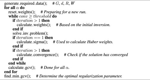
Applying regularization necessitates choosing a value for the regularization parameter. This is done automatically for each epoch using Generalized Cross-Validation (GCV) (Aster et al., 2013a) to ensure reproducibility and reduce human bias. The optimal value for the regularization parameter can be found by solving the inverse problem, Eq. 8, for a series of α-values and evaluate the GCV score, Eq. 10 where N is the number of observations. The optimal value of α is related to the lowest GCV score. As this approach can be computational very heavy, we implemented a simple steepest descent algorithm to minimize unnecessary computations.
In addition to reducing the model 2-norm the inverse problem is constrained by truncating the SH-degree at 40 resulting in 1,680 model parameters. The model is further constrained by 1) using only n − m odd terms which enforces hemispheric symmetry. 2) truncating the SH-order at 3 under the assumption that the east/west gradient is more smooth than the north/south gradient (Laundal et al., 2016). As a result of these two constraints the amount of model parameters is reduced to 272.The combination of iterative reweighting and Tikhonov regularization has been sketched out in Algorithm 1.In order to evaluate the variance in the model solutions a bootstrapping approach was taken. The inverse problem for each group of events was repeated 50 times while resampling the events going into the solution with replacement. Predictions from the various model realizations thus provide a variance estimate.
Algorithm 1. Inversion scheme.
3.3 Equivalent currents
The equivalent horizontal ionospheric current (EHIC) can similarly be represented by a scalar potential (Laundal et al., 2016) and therefore expressed in terms of the same SH coefficients as in Eq. 4.
Here h is the height with respect to a where the potential is evaluated. It is important to point out that Eq. 11 is the current potential expressed by the external magnetic field and h is therefore set to 110 km.
Evaluating the horizontal gradient of Ψ gives the EHIC.
Where
where β is the Hall and Pedersen conductance ratio and assumed to be constant. Equation 13 can be written in terms of Ψ by applying the relation from equation 34 in Sabaka et al. (2014).
β is still unknown and will later be assumed to be 1 resulting in what we will refer to as equivalent field aligned currents (EFACs). Thus providing estimates of the EHIC and EFAC in terms of SH coefficients.
4 Results
A rapid increase in Pd can cause a SC which is commonly decomposed into two main parts; the low/mid and high latitude geomagnetic response, Eq. 1, with varying spatial and temporal scales. Madelaire et al. (2022) carried out a superposed epoch analysis of the SMR and PCN index in order to examine these geomagnetic responses. In this study we carry out a superposed epoch analysis using SH modeling. With this approach we create a continuous model, in space, based on multiple events allowing us to estimate magnetic field perturbations and ionospheric equivalent currents. In this section we 1) present model results prior to onset to illustrate the methods ability to recreate IMF and dipole tilt dependent current patterns and 2) examine incoherent and coherent high latitude ionospheric responses and the dependence on IMF orientation and dipole tilt.
4.1 Prior patterns
This study builds on the premise that a superposed epoch analysis using a spherical harmonic modeling technique is capable of robustly reproducing the underlying pattern common for a majority of events in a group. As an initial assessment Figure 1 shows the mean and standard deviation of the external radial magnetic field perturbation Br across all 50 model realizations at epoch −5 (5 min prior to onset) for all 12 event groups above 50° mlat (magnetic latitude). The figure is divided into three rows indicating dipole tilt and four columns indicating IMF clock angle. The magnitude of the model predictions vary significantly across groups and the maps have therefore been given individual colorbars. The number in the upper right corner of each map indicate the maximum of their respective colorbars, in units of nT.
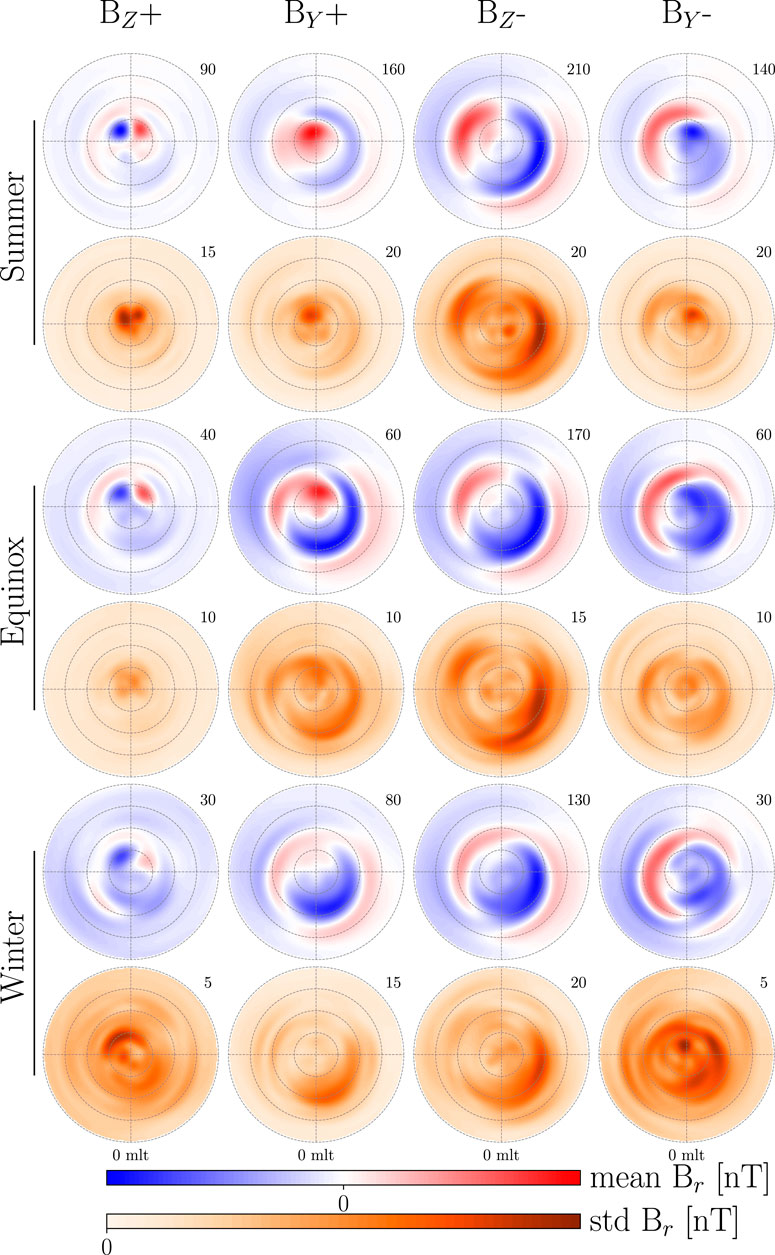
FIGURE 1. Illustration of the average model and its variation 5 min prior to onset. Each map shows either the mean or standard deviation of Br as predicted by the 50 model realizations. The number in the upper right corner of each map indicates the magnitude of the colorbars for that specific map in units of nT. The columns and rows indicate the IMF clock and dipole tilt angle, respectively.
Maps of the mean are in good agreement with previous studies on current patterns and their dependency on IMF clock angle and dipole tilt (Cowley and Lockwood, 1992; Pettigrew et al., 2010; Weimer, 2013; Laundal et al., 2018). Predictions during summer are of higher magnitude than equinox and winter mainly as a result of variations in sunlight-induced conductivity and auroral precipitation with decreasing dipole tilt (Moen and Brekke, 1993; Liou et al., 2001). During BZ+ there are strong NBZ currents and overall stronger currents on the duskside as a result of co-rotation (Förster et al., 2017). During BZ-region 1 and 2 (R1/R2) currents are strong as a result of reconnection on both day and nightside giving rise to a two-cell current pattern. During BY± conditions the dawn and dusk cells become more circular or crescent as a result of the dayside reconnection geometry, giving rise to alternate current paths.
Variation between model realizations is generally low, but can become large near the edges of current cells as a result of a varying latitudinal extent of the cells. The variations might be reduced if the magnitude of the IMF and increase in Pd was taken into account when creating the event groups.
4.2 High latitude geomagnetic response
The geomagnetic response is divided in two, Eq. 1. DP is further divided into PI (preliminary impulse) and MI (main impulse), Eq. 2, representing two sets of transient convection vortices. The resulting magnetic perturbation is superimposed on the pre-existing perturbation magnetic field shown in Figure 1. The signal from these transient convection vortices will in most cases be overshadowed by the dominant pre-existing signal. Figures 2, 3 show Ψ, Eq. 11, and EFACs (equivalent field aligned currents), Eq. 14, at epoch −5 and 5 (5 min before and after onset). The colored contours are EFACs, where red (blue) indicate an upward (downward) FAC, and Ψ is illustrated in terms of equipotential lines.
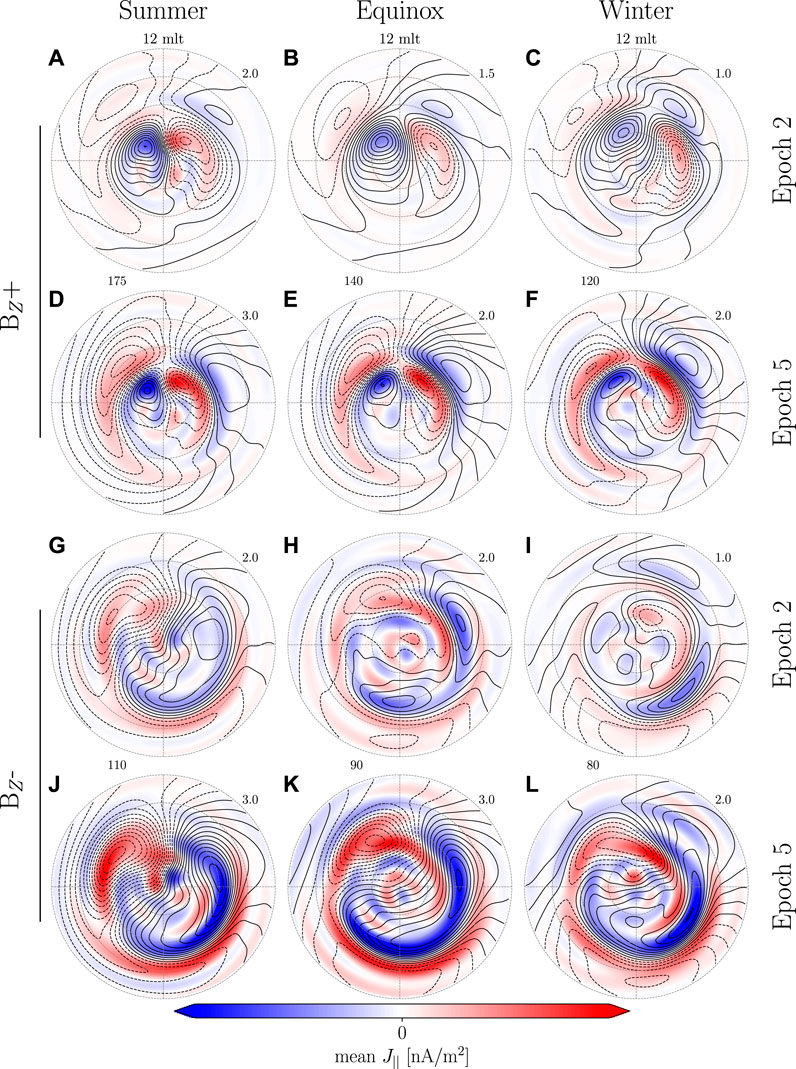
FIGURE 2. Maps of EHIC and EFAC 5 min before and after onset for the BZ groups. The colored contour indicates EFACs while Ψ is shown by the black equipotential lines. Each set of figures is described by the two numbers written between them. The first indicates the step size of Ψ in kA while the second indicates the maximum of their unique colorbar.
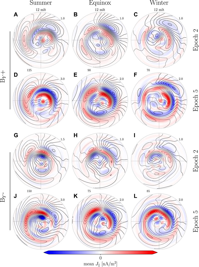
FIGURE 3. Similar to Figure 2, but for BY dominated IMF.
BZ+ models during equinox (Figures 2B,E) and winter (Figures 2C,F) show clear differences before and after onset. After onset the area around the NBZ currents intensifies and the current vortices extend towards the nightside. These vortices are confined by a second set of current vortices on their equatorward edge that have opposite orientation. The orientation, spatial extent and temporal evolution of these two set of current vortices are in agreement with previous case studies (Friis-Christensen et al., 1988; Moretto et al., 2000), statistical studies (Stauning and Troshichev, 2008) and MHD simulation studies (Slinker et al., 1999; Keller et al., 2002; Fujita et al., 2003a,b, 2005; Ridley et al., 2006; Samsonov et al., 2010; Samsonov and Sibeck, 2013; Shi et al., 2014; Welling et al., 2021). For all other event groups the general magnitude increases, but no transient response is observed (Figures 2A,D,G–L and Figures 3A–L). One factor that could play a role in the lack of a transient response is the increased dayside reconnection which enhances the preexisting convection pattern. The lack of a visible transient response is likely due to stronger pre-existing convection as a result of dayside reconnection.
4.2.1 Incoherent ionospheric response
In this section we attempt to look past the pre-existing magnetic field in order to examine the temporal evolution of the transient ionospheric response. This is more easily achieved by summarizing it by a single parameter. Here we use ΔΨ, the maximum difference in the current potential given by Eq. 11. Under normal circumstances the potential will be bi-modal with the global min/max coinciding with the current pattern allowing for easy determination of the maximum difference. Changes to the system will often manifest themselves as an increase or decrease in ΔΨ making it convenient for an analysis of the temporal evolution. Figure 4A shows the mean ΔΨ across all model realizations along with the 90% confidence interval. The time series was set to zero with respect to when the response initiates. The time at which the response initiates was determined using the rise time algorithm described by Madelaire et al. (2022). The algorithm also provides the peak (when the time series begins to plateau) allowing for the rise time to be determined.
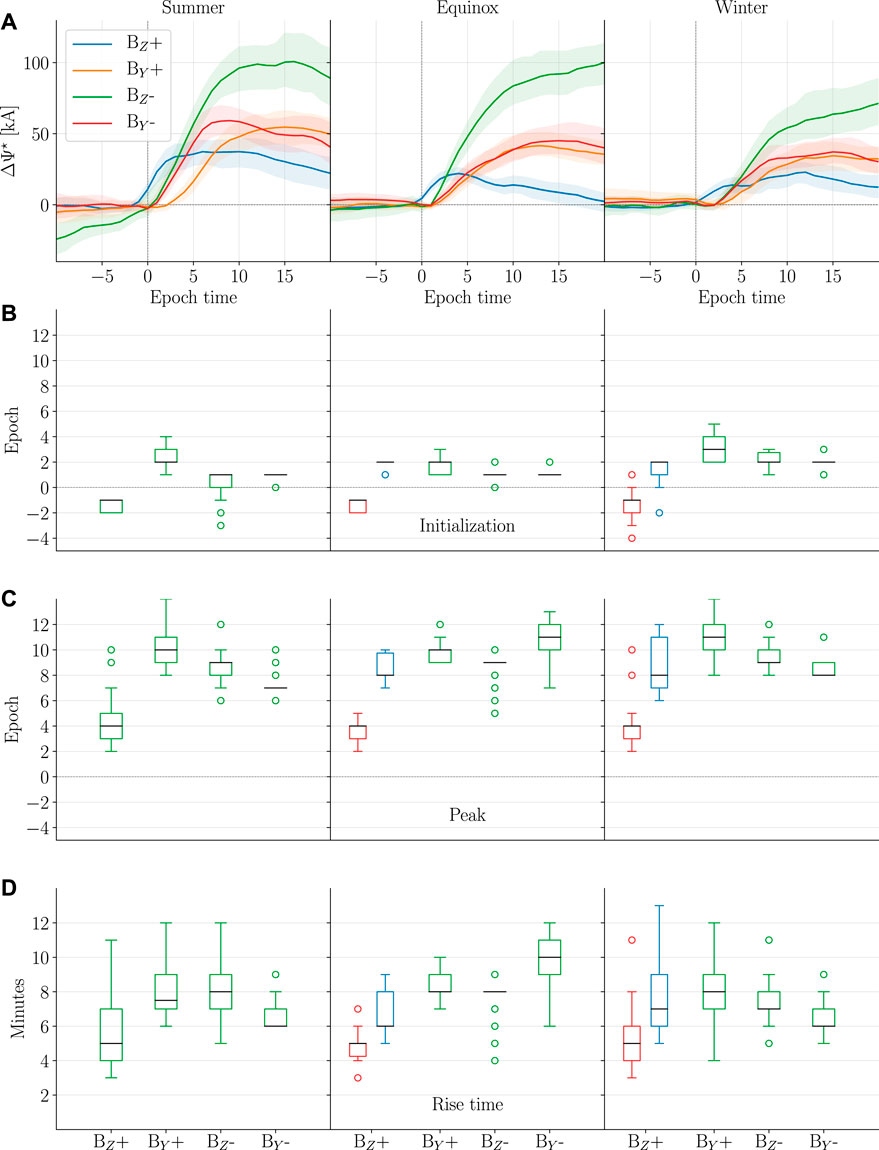
FIGURE 4. (A) Time series of ΔΨ for all 12 groups. The mean and 90% confidence interval across all 50 mode realizations is shown as a solid line and a shaded area, respectively. The time series was set to zero with respect to when the response initiates indicated by the asterisk on the y-axis. (B–D) Summary of statistics related to Figure 4A shown as box plots. (B) shows the epoch at which response initiates for the 12 groups. (C) shows when the ΔΨ time series peaks. (D) shows the rise time [difference between (A and B)]. During equinox and winter BZ+ is given by two (red and blue) boxplots which are related to a decomposition illustrated in Figure 5.
The shape, size and temporal evolution changes significantly with IMF clock angle and dipole tilt. In the rest of this section we take a closer look at the characteristics of Figure 4A.
4.2.1.1 Initialization
The epoch at which ΔΨ, in Figure 4A, begins to increase is illustrated as box plots in Figure 4B. The red and blue box plots relate to a decomposition done later in this section and the reader should disregard the blue box plot for now. The signal initiates around epoch 1–3 for all event groups except for BZ+ groups where the initialization occurs around epoch −2 to −1.
Determining ΔΨ is normally easy due to the bi-modal nature of Ψ. However, when multiple cells of similar magnitude grow and decay, as is the case for BZ+ during equinox and winter, the global min/max will jump around thus making the current method invalid. In these two cases we observed an increase in and around the NBZ cells, consistent with the PI (preliminary impulse), followed by an increase at 65°–75° mlat similar to R1/R2 starting on the dayside, consistent with the MI. We constrained the area within which ΔΨ was computed so as to separate the PI and MI. The PI was isolated by evaluating Ψ above 72° mlat and between 6 and 18 mlt (magnetic local time). The MI was isolated by evaluating Ψ between 65° and 80° mlat. Separate constraints were applied to the dawn and dusk cell due to an asymmetric response which will be further discussed in Section 4.2.2. At dusk Ψ was evaluated between 12 and 18 mlt while dawn was constrained to 6–12 mlt until epoch 5 whereafter it was relaxed to 0–12 mlt. The result of hard-coding where Ψ was evaluated allows for the separation of the two responses as shown in Figure 5. Here the mean PI (MI) is shown in red (blue) with a 90% confidence interval, and the maximum of the two is shown in black. We have labeled the two time series PI and MI as the current vortices observed correspond to the expected orientation and location of the convection vortices associated with PI and MI.
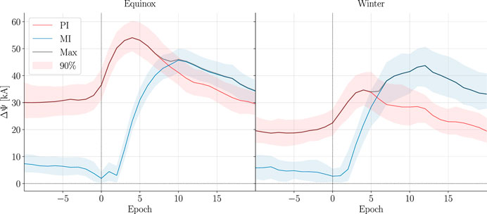
FIGURE 5. Decomposition ΔΨ for BZ+ during equinox and winter into PI and MI.
Returning to Figure 4B the PI (MI) is shown with red (blue) box plots. The PI values fit very well with those determined for BZ+ during summer where the response near the NBZ cells is dominant. The MI initialization fits very well with the initialization of ΔΨ for all other IMF clock angles. One might question why there is no PI for non-BZ+ groups. This is likely because the PI occurs poleward of the global min/max where ΔΨ is evaluated and its magnitude is not large enough to shift their location.
4.2.1.2 Peak and rise time
The peak and rise time of ΔΨ are shown in Figures 4C,D. For BZ+ the peak occurs around epoch 4 while for all other IMF conditions it occurs around epoch 7–11. The difference is not surprising considering how clearly the PI can be observed during BZ+. The results are consistent with the superposed epoch analysis of the PCN index conducted by Madelaire et al. (2022). The rise time for the PI is around 5 min while it is 6–10 min for the MI. When comparing Figures 4B–D, the largest source of variation in rise time is from the peak determination. This is consistent with Takeuchi et al. (2002) who studied the rise time of the low/mid latitude geomagnetic response and found it to be around 2–10 min with one event reaching 30 min, presumably due to a highly inclined shock normal.
4.2.1.3 Magnitude and decay
The average increase in Pd across event groups is of similar size, one might therefore assume that the magnitude of the geomagnetic response would be of similar magnitude across all IMF groups in a particular season. Comparing ΔΨ within the individual seasons shows BZ-to have a magnitude around 2 (3) times larger than BY± (BZ+). The solar wind-magnetosphere coupling efficiency is highly dependent on the IMF clock angle (Newell et al., 2007) and it is therefore no surprise that ΔΨ is significantly larger for BZ-due to dayside reconnection.
The ΔΨ ratio between summer and winter is ∼1.8 for all IMF clock angles. The ratio of the PI for BZ+ is 2.4 indicating a much higher seasonal dependence. Samsonov et al. (2010) studied the effects of an interplanetary shock using a MHD simulation and concluded that the PI was associated with lobe reconnection. If this finding is true the larger variation in the PI can be controlled partly by dipole tilt as it has a large impact on the lobe coupling efficiency (Reistad et al., 2019).
Similar to the magnitude, the decay is IMF clock angle dependent. The decay during BZ+ is quicker compared to other event groups. The BY± groups plateau or decay slowly while BZ-plateau or trend upwards. The longer lived response for BY± and BZ-is most probably a consequence of increased dayside reconnection brought on by the new pressure balance.
4.2.2 Northward IMF case
In Section 4.2.1 we examined the ionospheric response to rapid increases in Pd and found dependencies on both IMF clock angle and dipole tilt. Here we examine the temporal evolution using the model during BZ+ as the transient event is strongest relative to the background for these environmental conditions.
The decomposition of ΔΨ in Figure 5 illustrates the magnitude of PI and MI along with their temporal extent. The decomposition was made by evaluating the local min/max of Ψ. The positions used in that calculation can be visualized to show how the cells move and the variation between model realizations. Figure 6 shows the location of the current potential min/max in orange/purple dots. Superimposed is the average path where the green (red) dots indicate the beginning (end). The PI is shown from epoch −2–10 and the MI is shown from 0 to 15. It is clear that the center of the PI current vortices and the MI vortex at dusk do not move much. However, the MI at dawn moves from around 10 to 6.5 mlt between epoch 2–8 (6 min) at 67° mlat leading to a westward velocity of 6.3 km/s. This is similar in size to the estimates of 3–5 km/s by Friis-Christensen et al. (1988) and 5 km/s by Slinker et al. (1999). After epoch 8 the center jumps from 6 to 2 mlt as the current vortex weakens and becomes indistinguishable from the pre-existing feature on the night side.

FIGURE 6. Illustration of the PI and MI current vortex centers resulting from the decomposition of ΔΨ during BZ+ Winter in Figure 5. The poleward (equatorward) purple/orange dots indicate convection cell centers for PI (MI) across all 50 model realizations between epochs −2–8 (0–10). The black lines indicated the average path of the convection cell where the green and red dots indicate the start and end, respectively.
Figures 7, 8 show maps of EHIC and EFAC superimposed. Here model predictions are shown with 1–min resolution spanning epoch −1–6 and then with 2–min resolution from epoch 6–14. Before onset there is a set of NBZ cells with centers located around (9 mlt, 80° mlat) and (14 mlt, 82° mlat). There appears to be virtually no westward electrojet, while there is an eastward electrojet, possibly due to co-rotation (Förster et al., 2017). On the nightside there are 2 cells located around (1 mlt, 75° mlat) and (21 mlt, 70° mlat) and are likely related to nightside reconnection.
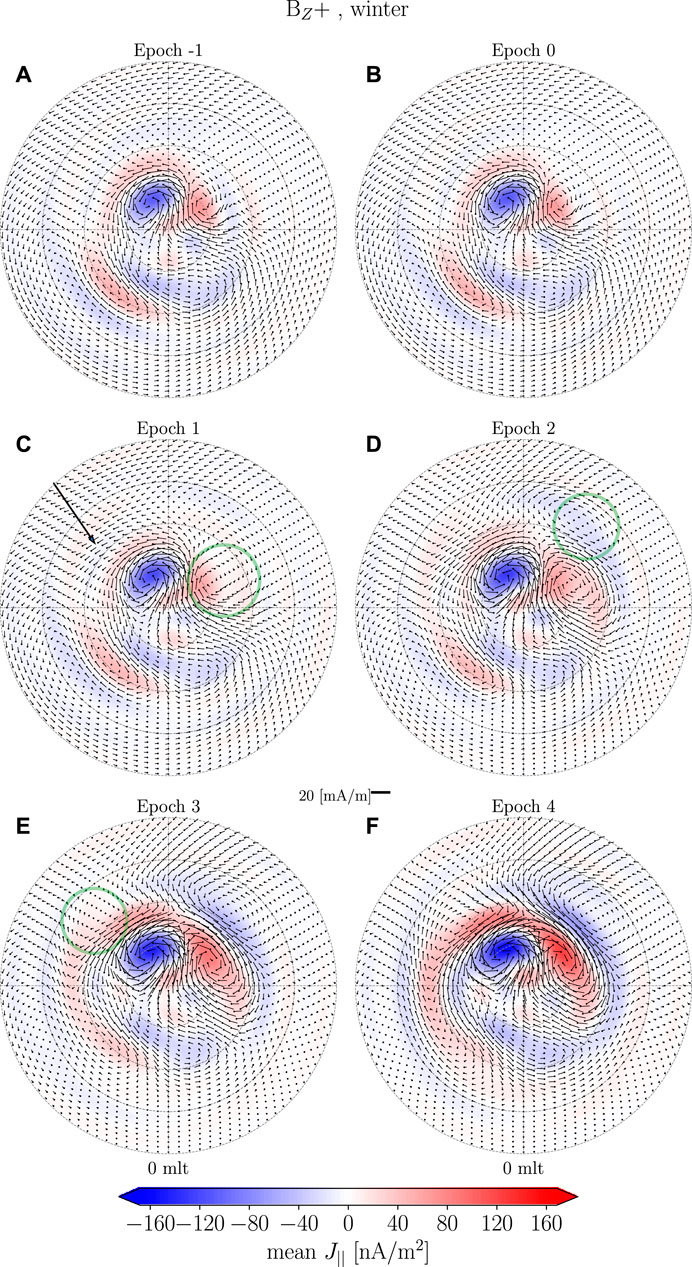
FIGURE 7. Maps of BZ+ during Winter from epoch −1–4. The contours and arrows indicated EFACs and EHICs, respectively.
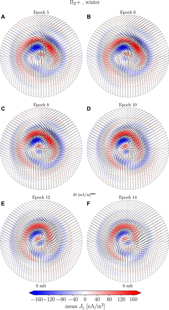
FIGURE 8. Maps of BZ+ during Winter from epoch 5–14. The contours and arrows indicated EFACs and EHICs, respectively.
There is no apparent difference when comparing epochs −1 and 0 (Figures 7A,B). One minute after onset, Figures 7A,C small intensification is observed at pre- and post-noon around 65°–80° mlat as indicated by the annotations. Two minutes after onset, Figure 7D, the equatorward boundary of the pre-noon structure has moved poleward to 70° mlat and merged with the pre-existing NBZ cell with its center located around (8 mlt, 78° mlat). Additionally, a current vortex with opposite orientation has appeared at (10 mlt, 65° mlat). At post-noon we see a general intensification of the pre-existing current pattern. It is possible that the pre-existing eastward electrojet obscures the PI which therefore is manifested as a general increase of the pre-existing current pattern. Between epoch 3 and 4, Figures 7E,F, the PI current vortices intensify, move poleward and start draping towards the nightside while their centers do not move. At dawn the MI current vortices intensifies, extending toward the night side while its center moves 1–2 MLT westward. At dusk the center of the MI current vortex appears and as it intensifies it moves poleward, from (15 mlt, 65° mlat) to (15 mlt, 70° mlat), and merges with the pre-existing nightside current vortex. Between epoch 5 and 6, Figures 8A,B, the PI cell intensifies while their equatorward extent decrease. At the same time the MI also intensifies and the center of the dawnside vortex moves westward. The duskside MI current vortex becomes more well defined and moves poleward. Between epoch 8 and 10, Figures 8C,D, the PI decreases in intensity and at dawn the PI vortex merges with the MI vortex at dusk. The center of the MI vortex at dawn moves westward and becomes less well defined. At dusk the MI cell intensifies and moves slightly westward towards the noon meridian. Between epoch 12 and 14, Figures 8E,F, the PI response continues to decrease in strength. The MI response slowly disappears at dawn while it remains strong at dusk.
In our examination of the BZ+ during winter a transient high latitude geomagnetic response was observed and will be discussed further in Section 5.
4.2.3 Coherent ionospheric response
Despite the lack of a visible transient response in a majority of the event groups it might very well still be there, hidden under a more dominant current pattern. A weak transient signal can be examined by evaluating the relative change as long as the contribution from the change of the transient signal is larger than that of the background signal.
In Figures 2E,F the MI-associated current vortices appears to extend far equatorward. This, to some extent, is an artifact caused by how DL geomagnetic response maps into the horizontal magnetic field at subauroral latitudes, mainly the north/south component, resulting in what appears to be large scale east/west aligned ionospheric current. We remove this effect by approximating the magnetic perturbation from magnetospheric sources as an external dipole field. The external dipole field can be seen as uniform magnetic field in
which except for a sign difference is the same as the SH expansion of the external magnetic field to degree 1 and order 0. Bm is determined at each epoch as the average of 1,000 model predictions at 30° mlat that are evenly spaced in mlt. The effect of the magnetospheric compression is then isolated by subtracting a baseline prior to onset. Finally, a corrected SH model is created,
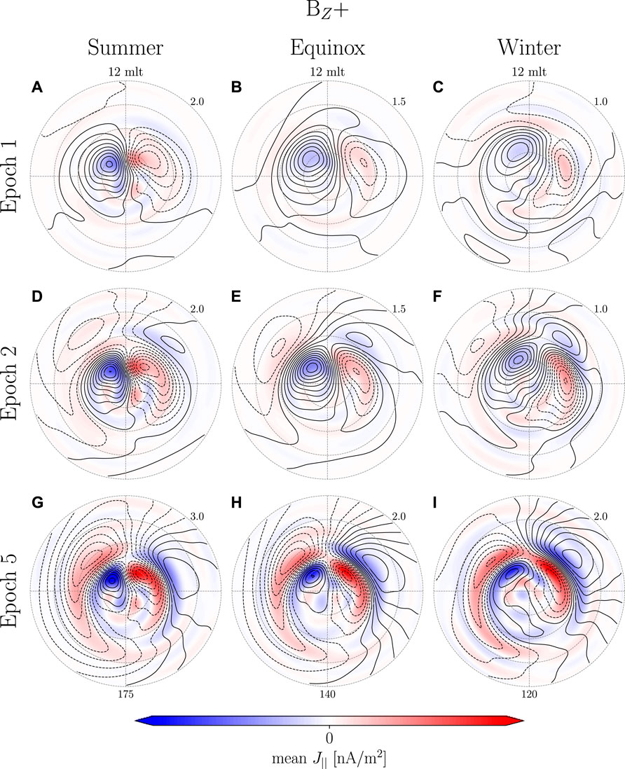
FIGURE 9. Relative change from epoch −2 to epoch 1, 2, and 5 for BZ+. The blue/red contour illustrates EFAC while the black contour is Ψ. Each column represents a specific dipole tilt range and the number at the bottom of each column is the maximum value of the associated colorbar in units nA/m2. The number in the top right of each map is the step size of the black contour in kA.
When comparing BZ+ between Figure 9 to Figure 2A–F it is clear that the transient high latitude response shows very little dipole tilt dependence. At epoch 1 (Figure 9A–C) only the PI is present. At epoch 2 (Figure 9D–F) the MI starts forming around 60°–65° mlat. At epoch 5 (Figure 9G–I) both PI and MI increase in magnitude and the center of the MI vortex at post-noon has moves poleward by 5° mlat while the vortex at pre-noon moves westward.
The BY± groups at epoch 1 (Figures 10A–C and Figure 11A–C) show PI current vortices. They are not as well defined when comparing with BZ+, but there does not appear to be any favoring of one vortex over the other as might be expected when comparing BY+ and BY-. At epoch 2 (Figures 10D–F and Figures 11D–F) the PI moves slightly poleward as the MI forms on its equatorward edge. In some cases, Figures 10D, 11D,E, one of the PI vortices disappear or merge with one of the MI vortices. This might be attributed to the model’s spatial resolution, the fact that we are looking at a relative change or the combination of northward and southward IMF in BY± groups causing higher variation between events close to the pole. At epoch 5 (Figures 10G–I, 11G–I) the PI is almost completely gone and the MI is well defined with the exception of BY+ winter where no clear MI current vortex appear on the dusk side. Under these environmental conditions it is also only the MI vortex on the dawnside that moves toward the nightside.
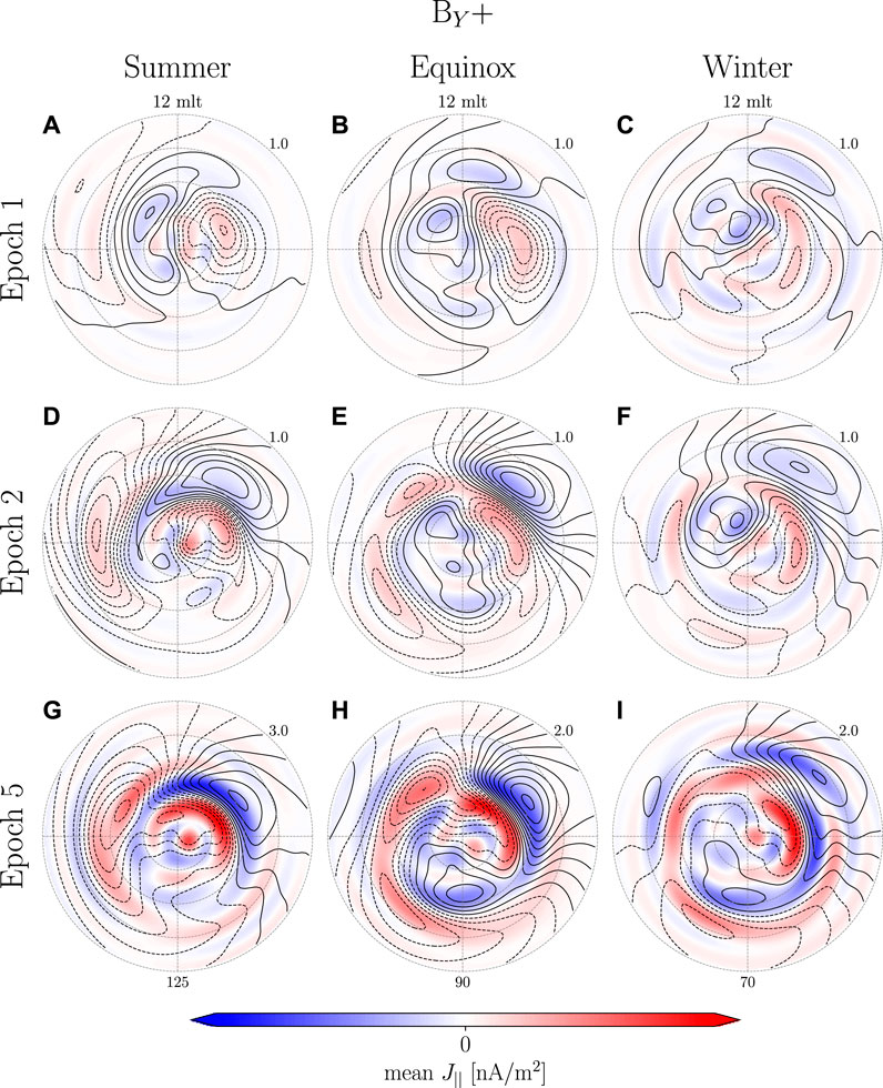
FIGURE 10. Similar to Figure 9, but for BY+.
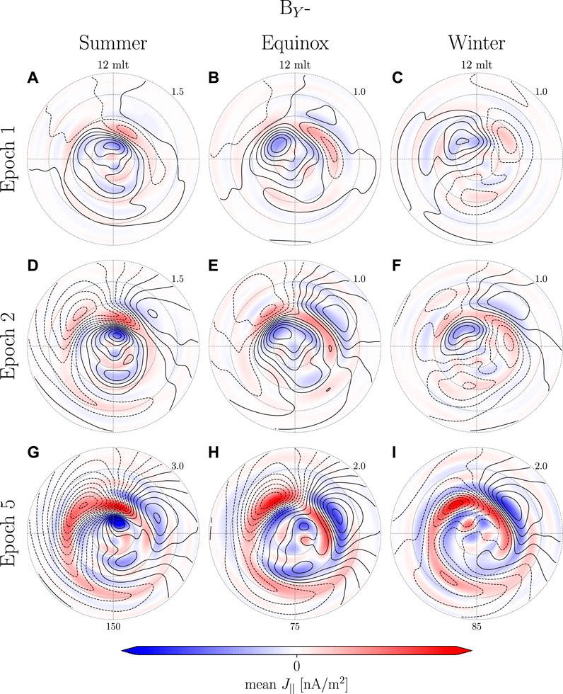
FIGURE 11. Similar to Figure 9, but for BY-.
The current potential for BZ- at epoch 1 (Figures 12A–C) is highly variable, i.e. many local min/max, and it is therefore difficult to associate any of the structures to PI or MI. During summer (Figures 12A,D,G) the current pattern is very similar to the expected current pattern during southward IMF (Laundal et al., 2018). The center of the 2 cells are shifted towards the dayside indicating some similarity to the MI current vortices. During equinox and winter current vortices appear on the night side at epoch 1 and increase in strength at epoch 2 (Figures 12B,C,E,F). At epoch 2 during equinox (Figure 12E) two MI associated vortices appear on the dayside; one on the dawnside and another very close to noon on the duskside. At epoch 5 (Figure 12H) the dawnside MI vortex merges with that on the nightside. The same can be observed during winter, however, the post-noon current vortex first appears at epoch 5 (Figure 12I). Common for all BZ-groups is a general lack of the PI current vortices and a very strong nightside geomagnetic response possibly associated with dipolarization of the tail magnetic field as observed by Lee and Lyons (2004).
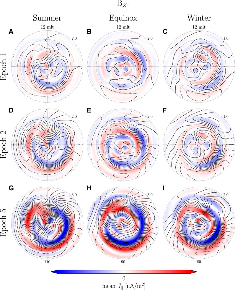
FIGURE 12. Similar to Figure 9, but for BZ-.
5 Discussion
In our examination of the transient high latitude response we looked closely at the model for northward IMF during winter as these are the conditions under which the transient response is strongest relative to the background. The model shows vortices that evolve on a minute time scale. The spatial extent of the vortices vary with time, however, the center of the vortices tend not to move except for the MI-associated vortex on the dawnside which moves westward with an estimated velocity of 6.3 km/s. The shock impact angle is surprisingly not one of the factors controlling the motion of the MI-associated vortices at dawn and dusk. Our reasoning is as follows. Madelaire et al. (2022) argued that the majority of the events in their list of rapid increases in Pd are not interplanetary shock. It is therefore likely that our results represent an average impact angle that is skewed toward dusk, in agreement with the statistical survey of rapid solar wind pressure changes presented by Dalin et al. (2002). In contrast the case study of Moretto et al. (2000), which used the AMIE technique to model the ionospheric response of an inclined shock arriving first at the dawn side, also found that the MI-associated convection vortex at dusk did not move, while that at dawn did. If the impact angle controlled which vortex convects toward the nightside, the response of the vortices reported by Moretto et al. (2000) would presumably be opposite the observed response; that is, the dusk vortex would have moved toward the nightside while the dawn vortex remained stationary. Existing simulation-based studies of interplanetary shocks unfortunately do not lend much insight (Slinker et al., 1999; Keller et al., 2002; Fujita et al., 2003a,b; Ridley et al., 2006; Samsonov et al., 2010; Welling et al., 2021): while they universally show a symmetric ionospheric response across the noon-midnight meridian with both MI cells moving anti sunward, all have been carried out with an interplanetary shock aligned with the Sun-Earth line.
5.1 Coherent high-latitude response
A coherent transient high latitude geomagnetic response is observed for all groups when examining the relative change with respect to epoch −2 (Figures 9–12). When comparing different groups we find the EFAC magnitude and PI current vortices to be more dominant during BZ+ likely due to a higher contribution from lobe reconnection. During BZ-there is a general lack of PI and the MI is poorly resolved due to a significant enhancement of the pre-existing current pattern. The appearance of MI current vortices during BZ+ and BY± is very consistent. We estimate the westward velocity of the dawnside associated MI current vortex based on epoch 2–5 (Figures 9–11) to be between 3.6 and 7.8 km/s with a mean of 5 km/s and a standard deviation of 1.4 km/s. The initial appearance of the MI current vortex on the dawnside occurs at (9.3 ± 0.5 mlt, 64.8° ± 1.5° mlat) while it on the duskside occurs at (15.3 ± 0.9 mlt, 65.8° ± 2.5° mlat) with the majority of the mlt variation caused by Figure 11D.
The SH model is a global representation of the magnetic potential. It is important to understand the benefits and shortcomings of the method such that results can be interpreted in the correct context and improvements or alternatives might be proposed. The spatial resolution of any modeling method will partly depend on data coverage. When using ground magnetometers the data coverage is seldom uniform and the spatial resolution is highly dependent on the area with the lowest data density. By combining multiple events, as done here, we can achieve much denser data coverage resulting in a better spatial resolution. Combining multiple events generates inconsistencies as observations that are spatially very close can vary significantly. The variation is reduced by only combining events thought to be of similar nature. The model will inevitably be an average highlighting features common for all the events. We have tried to quantify the variation in our model using bootstrapping (Figure 1), but in order to understand how and why events vary from the average they need to be analyzed individually. The spherical elementary current system technique (Amm et al., 2002) is ideal for analyzing single events as it is not globally defined and can take advantage of the regions with dense data coverage. This method is implemented by Laundal et al. (2022); they combine magnetic perturbation and convection measurements from space and ground with conductance measurements via ionospheric Ohm’s law to significantly improve data coverage and information retrieved. This will be a very useful tool when the EZIE satellite mission (Laundal et al., 2021) launches in the near future providing measurements of the magnetic field in the mesosphere. In the future we intend to carry out a regional analysis of events to study their variation in more detail.
5.2 Huber weights
A superposed epoch analysis assumes a certain level of comparability between events which we in practice achieve by imposing criteria on IMF clock angle and dipole tilt. It is obvious that there will be differences between events and at times so much so that individual events can be considered outliers. When solving the inverse problem the imposed spatial relationship, inherent in SHs, will force the solution toward the typical event and thereby automatically reduce the relative importance of certain data. Adding iterative reweighting allows for a fine tuning of the fit as the influence of outliers are weighed down and the inversion repeated. The term outliers is often used synonymously with measurement errors, but here refer to events behaving differently from the majority. In practice, the outliers are weighed down using Huber weights which are determined as part of the iterative procedure.
The Huber weights can be used to analyze how consistent the data selection is and if outliers are correlated with certain environmental parameters. Figure 13 visualizes the average Huber weight for each event using data-points above 50° mlat with respect to certain environmental parameters. Each dot represents an event and the size of the dot indicates the weight of that specific event illustrated by the scale of red dots in the upper left corner; a large (small) dot indicates an event that has been weighed low (high) in the inversion. Figures 13A,B show how the weight relates to the Newell coupling function (Newell et al., 2007) before onset, the SYM-H index before onset and
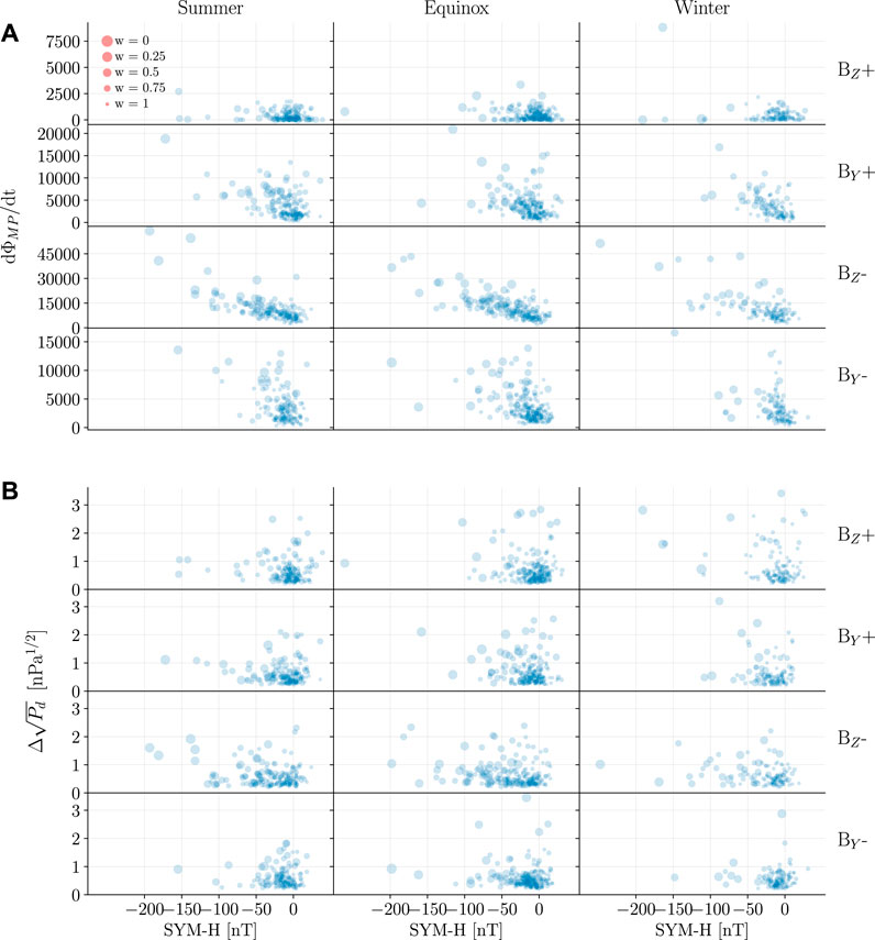
FIGURE 13. Huber weights at epoch 5 for each event. In (A) illustrated as function of the Newell coupling function and SYM-H before onset and in (B) as function
These figures are not intended to be employed in determining which parameters to use for grouping events, but are rather an illustration of how information about individual events can be extracted from a superposed epoch analysis. Additionally, they serve as an illustration of how data selection occurs prior to and during the modeling process.
5.3 Low/mid latitude geomagnetic response
A benefit of a global model is the possibility of examining the high latitude impact on low/mid latitude perturbations. Changes in
Russell et al. (1994a) did a statistical analysis of the linear relationship during interplanetary shocks and found the slope to be 18.4 nT/nPa1/2 at Earth’s surface which includes a 50% markup due to ground induced currents. This estimate was given for northward IMF and should be reduced by 25% (13.8 nT/nPa1/2) during southward IMF (Russell et al., 1994b). The superposed epoch analysis by Madelaire et al. (2022) was based on the SMR index and found the average relationship to be around 15 nT/nPa1/2 during northward IMF and around 12 nT/nPa1/2 for southward IMF. Additionally, Madelaire et al. (2022) found a dawn-dusk asymmetry in the SMR index as well as a noon-midnight asymmetry for southward IMF.
The SH models are essentially a weighted average of the events in each group expressed in terms of SH surface waves. Their performance can be compared to the results of Madelaire et al. (2022) by testing if they can recreate their results. The results of the superposed epoch analysis of the SMR index by Madelaire et al. (2022) is reproduced in Figure 14A to facilitate comparison later. The SMR index was recreated using the SH models; the northward component of the magnetic field perturbations are calculated using the internal and external model for each of the 50 realizations between the equator and 50° mlat. The model predictions are made at the same location as the data that went into the models. A latitudinal correction similar to that of the SMR index was applied (Newell and Gjerloev, 2012). The model predictions from each realization are scaled with the median of
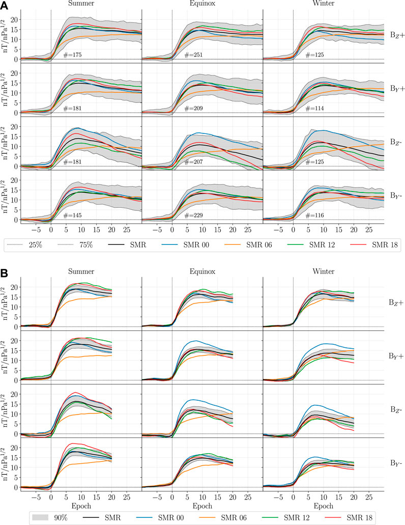
FIGURE 14. Comparison between the superposed epoch analysis of the SMR index by Madelaire et al. (2022) and the recreated SMR index from the SH models. (A) Similar to Figure 9 of (Madelaire et al., 2022). (B) The recreated SMR index where the solid lines indicate the mean of SMR and its local time components. The gray area indicates a 90% confidence interval of the global SMR. The SMR time series for each model realization has been scaled with respect to the median increase in
The recreated SMR index is shown in Figure 14B. The expected step-like increase is reproduced. The magnitudes of SMR range from 12 to 19 nT/nPa1/2 which is slightly larger than the averages provided in Figure 14A. The dawn-dusk difference is also reproduced which is most pronounced during summer. Comparing Figures 14A,B suggests that the SH models are sufficient to reproduce the expected geomagnetic response observed on ground which is an indication that the modeling scheme performs well.
The latitudinal profile of the recreated SMR for BZ+ is shown in Figure 15. The first 5 rows show 5 latitude bands between 0° and 50° mlat. The last row is identical to the first row of Figure 14B for more easy comparison. It is clear that the dawn-dusk asymmetry is most pronounced between 40° and 50° mlat. This suggests it is an ionospheric source and not magnetospheric, given its small spatial extent. A recent study (Zhou and Lühr, 2022) investigated SCs with an immediate and strong activation of the westward electrojet. However, they concluded that it required southward IMF preceding the SC. The lower magnitude at dawn between 40° and 50° mlat could reflect the ionospheric vortices generated at high latitude. The seasonal dependence would then be a result of seasonal variations in conductance varying the strength of the high latitude currents and thus the latitudinal extent of their magnetic perturbation.
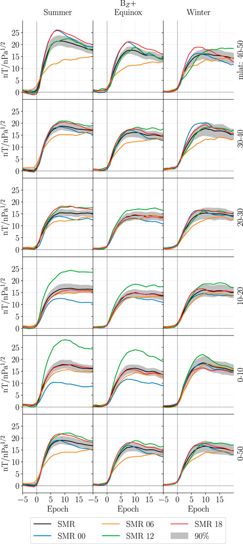
FIGURE 15. A latitudinal profile of the reproduced SMR for BZ+ during all seasons. The first five rows show contributions from five latitudinal regions between 0° and 50° mlat. The last row shows SMR for the entire latitudinal region which is identical to row 1 of Figure 14B.
In the region closest to the equator, 0°–10° mlat, a noon-midnight asymmetry is observed which is present for all IMF clock angles (only BZ+ shown). The geomagnetic response on the dayside (nightside) tends to be stronger (weaker) than at dawn and dusk. The small latitudinal and longitudinal extent of the dayside/nightside (SMR 12/00) enhancement suggests an ionospheric source. A seasonal dependence is observed as the asymmetry almost disappears during winter. There are several possible explanations for this; Kikuchi (1986); Kikuchi et al. (2001); Kikuchi (2014) proposed that the potential difference at high latitude would be transported toward the equator in an Earth-ionosphere waveguide. In this frame the increased equatorial perturbation is caused by Cowling conductivity. However, Tu and Song (2019) argued against this idea as the waveguide should transport the electric field with the speed of light and the observed delay between high and low latitude is in the order of minutes. Movement of the Sq foci is thought to be responsible for the semiannual variation of the equatorial electrojet (Tarpley, 1973). The seasonal variation is not a modulation of the magnitude, but rather a latitudinal shift along with the Sq foci. Unfortunately, we are not able to test this hypothesis with our model as they are only based on data from the northern hemisphere. It is also possible that there is no hemispheric asymmetry and the seasonal variation is an artifact caused by the event occurrence probability being skewed toward a certain UT range for different dipole tilt angles due to the offset between the geomagnetic and geographic poles. Specifically, events are more likely to occur between 0 and 12 (12–24) UT for positive (negative) dipole tilt. Trivedi et al. (2005) showed that the magnetic perturbation due to SCs measured close to the south atlantic magnetic anomaly are stronger than elsewhere. It is therefore possible that the dipole tilt dependence of the magnetic perturbation at equator latitude simply is due to longitudinal variations in the equatorial electrojet.
It is clear that the geomagnetic response between 10° and 40° mlat is very similar while magnetometer observations between 0°–10° and 40°–50° mlat are under high influence of ionospheric sources. This consideration was taken into account in the development of the Dst index (Sugiura, 1964; Sugiura and Kamel, 1991) and it is therefore curious that it is not taken into account in the SYM-H and SMR index (Iyemori et al., 2010; Newell and Gjerloev, 2012). We do not attempt to understand the origin of the contamination pointed out here as that should be done in a future study using data directly from the magnetometer stations and not our SH models.
6 Conclusion
In this study we carried out a superposed epoch analysis of the transient high latitude geomagnetic response in the northern hemisphere to rapid increases in solar wind dynamic pressure using spherical harmonics. The analysis is based on the list of rapid solar wind pressure increases presented by Madelaire et al. (2022). A total of 2058 events were separated into 12 groups, Supplementary Table S1, based on IMF clock angle and dipole tilt. We found:
1. An incoherent geomagnetic response for a majority of the groups due to a dominant background signal; only during BZ+ equinox and winter was the transient response visible.
2. A coherent geomagnetic response showing the development of current vortices associated with PI and/or MI of the sudden commencement was observed for all groups when evaluating the relative change with respect to epoch −2.
3. The PI (MI) onset occurs ∼2 min before (after) the SYM-H defined onset and the rise time is 4–6 (6–11) min.
4. The pre-noon current vortex associated with the MI initially appears at (9.3 ± 0.5 mlt, 64.8° ± 1.5° mlat) and moves westward with a velocity of 5 ± 1.4 km/s until it reaches ∼6 mlt. Here it remains while it slowly decays and a new steady state current pattern emerges.
5. The post-noon current vortex associated with the MI initially appears at (15.3 ± 0.9 mlt, 65.8° ± 2.5° mlat) and does not move towards the nightside which is inconsistent with previously published models and MHD simulations.
6. The high latitude impact on the low/mid latitude perturbation results in significant contamination of the SMR index due to the inclusion of observations from 0° to 10° mlat and 40°–50° mlat.
The purpose of the study was to create a climatological analysis of the transient high latitude geomagnetic response. In the future we intend to examine how individual events in the 12 groups differ from each other and what the controlling environmental factors are.
Data availability statement
Publicly available datasets were analyzed in this study. This data can be found here: Event list (doi. org/10.5281/zenodo.6243103), Ground magnetic perturbation from SuperMAG.
Author contributions
MM is the primary author and carried out the analysis. KML and JPR helped set up the overall structure of the manuscript. All co-authors contributed to the discussions and provided editorial comment thus contributing to the article and approved the submitted version.
Funding
This work was funded by the Research Council of Norway (RCN) under contract 223252/F50. KL and JR were also funded by the RCN under contract 300844/F50. KL and SH were also funded by the Trond Mohn Foundation.
Conflict of interest
The authors declare that the research was conducted in the absence of any commercial or financial relationships that could be construed as a potential conflict of interest.
Publisher’s note
All claims expressed in this article are solely those of the authors and do not necessarily represent those of their affiliated organizations, or those of the publisher, the editors and the reviewers. Any product that may be evaluated in this article, or claim that may be made by its manufacturer, is not guaranteed or endorsed by the publisher.
Supplementary material
The Supplementary Material for this article can be found online at: https://www.frontiersin.org/articles/10.3389/fspas.2022.953954/full#supplementary-material
References
Amm, O., Engebretson, M. J., Hughes, T., Newitt, L., Viljanen, A., and Watermann, J. (2002). A traveling convection vortex event study: Instantaneous ionospheric equivalent currents, estimation of field-aligned currents, and the role of induced currents. J. Geophys. Res. 107, 1334. SIA 1–1–SIA 1–11. doi:10.1029/2002JA009472
Araki, T. (1994). A physical model of the geomagnetic sudden commencement (American geophysical union (AGU)). Sol. Wind Sources Magnetos. Ultra-Low-Frequency Waves,Geophysical Monogr. Ser., 183–200. doi:10.1029/GM081p0183
Aster, R. C., Borchers, B., and Thurber, C. H. (2013a). “Chapter four - tikhonov regularization,” in Parameter estimation and inverse problems. Editors R. C. Aster, B. Borchers, and C. H. Thurber. Second Edition (Boston: Academic Press), 93–127. Second edition edn. doi:10.1016/B978-0-12-385048-5.00004-5
Aster, R. C., Borchers, B., and Thurber, C. H. (2013b). “Chapter two - linear regression,” in Parameter estimation and inverse problems. Editors R. C. Aster, B. Borchers, and C. H. Thurber. Second Edition (Boston: Academic Press), 25–54. Second edition edn. doi:10.1016/B978-0-12-385048-5.00004-5
Burton, R. K., McPherron, R. L., and Russell, C. T. (1975). An empirical relationship between interplanetary conditions and dst. J. Geophys. Res. 80 (1896-1977), 4204–4214. doi:10.1029/JA080i031p04204
Chapman, S., and Bartels, J. (1940). Geomagnetism, 2. Oxford University Press. chap. 17. doi:10.2307/3606494
Constable, C. G. (1988). Parameter estimation in non-Gaussian noise. Geophys. J. Int. 94, 131–142. doi:10.1111/j.1365-246X.1988.tb03433.x
Cowley, S. W. H., and Lockwood, M. (1992). Excitation and decay of solar wind-driven flows in the magnetosphere-ionosphere system. Ann. Geophys. 10.
Curto, J., Araki, T., and Alberca, L. (2007). Evolution of the concept of sudden storm commencements and their operative identification. Earth Planets Space 59–xii. doi:10.1186/BF03352059
Dalin, P. A., Zastenker, G. N., and Richardson, J. D. (2002). Orientation of middle-scale structures in the solar wind plasma. Cosmic Res. 40, 319–323. doi:10.1023/a:1019838226629
Finlay, C. C., Kloss, C., Olsen, N., Hammer, M. D., Tøffner-Clausen, L., Grayver, A., et al. (2020). The chaos-7 geomagnetic field model and observed changes in the south atlantic anomaly. Earth Planets Space 72, 156. doi:10.1186/s40623-020-01252-9
Förster, M., Doornbos, E., and Haaland, S. (2017). The role of the upper atmosphere for dawn-dusk differences in the coupled magnetosphere-ionosphere-thermosphere system. Dawn-Dusk Asymmetries Planet. Plasma Environments,Geophysical Monogr. Ser. 10, 125–141. American Geophysical Union (AGU)), chap. doi:10.1002/9781119216346.ch10
Friis-Christensen, E., McHenry, M. A., Clauer, C. R., and Vennerstrøm, S. (1988). Ionospheric traveling convection vortices observed near the polar cleft: A triggered response to sudden changes in the solar wind. Geophys. Res. Lett. 15, 253–256. doi:10.1029/GL015i003p00253
Fujita, S., Tanaka, T., Kikuchi, T., Fujimoto, K., Hosokawa, K., and Itonaga, M. (2003a). A numerical simulation of the geomagnetic sudden commencement: 1. Generation of the field-aligned current associated with the preliminary impulse. J. Geophys. Res. 108, 1416. doi:10.1029/2002JA009407
Fujita, S., Tanaka, T., Kikuchi, T., Fujimoto, K., and Itonaga, M. (2003b). A numerical simulation of the geomagnetic sudden commencement: 2. Plasma processes in the main impulse. J. Geophys. Res. 108, 1417. doi:10.1029/2002JA009763
Fujita, S., Tanaka, T., and Motoba, T. (2005). A numerical simulation of the geomagnetic sudden commencement: 3. A sudden commencement in the magnetosphere-ionosphere compound system. J. Geophys. Res. 110, A11203. doi:10.1029/2005JA011055
Fukushima, N. (1969). Equivalence in ground geomagnetic effect of chapman-vestine’s and birkeland-alfven’s electric current systems for polar magnetic storms. Rep. Ionos. Space Res. Jap. 23 (1969), 219–227.
Fukushima, N. (1976). Generalized theorem for no ground magnetic effect of vertical currents connected with Pedersen currents in the uniform-conductivity ionosphere. Rep. Ionos. Space Res. Jpn. 30, 35–40.
Gjerloev, J. W. (2012). The supermag data processing technique. J. Geophys. Res. 117. doi:10.1029/2012JA017683
Glassmeier, K. H., and Heppner, C. (1992). Traveling magnetospheric convection twin vortices: Another case study, global characteristics, and a model. J. Geophys. Res. 97, 3977. doi:10.1029/91JA02464
Glassmeier, K. H., Hönisch, M., and Untiedt, J. (1989). Ground-based and satellite observations of traveling magnetospheric convection twin vortices. J. Geophys. Res. 94, 2520. doi:10.1029/JA094iA03p02520
Huang, C.-S. (2005). Variations of polar cap index in response to solar wind changes and magnetospheric substorms. J. Geophys. Res. 110, A01203. doi:10.1029/2004JA010616
Iyemori, T., Takeda, M., Nose, M., and Toh, H. (2010). Internal report of data analysis center for geomagnetism and space magnetism. Japan: Kyoto University.Mid-latitude geomagnetic indices asy and sym for 2009 (provisional)
Keller, K. A., Hesse, M., Kuznetsova, M., Rastätter, L., Moretto, T., Gombosi, T. I., et al. (2002). Global mhd modeling of the impact of a solar wind pressure change. J. Geophys. Res. 107, 1126. SMP 21–1–SMP 21–8. doi:10.1029/2001JA000060
Kikuchi, T. (1986). Evidence of transmission of polar electric fields to the low latitude at times of geomagnetic sudden commencements. J. Geophys. Res. 91, 3101. doi:10.1029/JA091iA03p03101
Kikuchi, T. (2014). Transmission line model for the near-instantaneous transmission of the ionospheric electric field and currents to the equator. J. Geophys. Res. Space Phys. 119, 1131–1156. doi:10.1002/2013JA019515
Kikuchi, T., Tsunomura, S., Hashimoto, K., and Nozaki, K. (2001). Field-aligned current effects on midlatitude geomagnetic sudden commencements. J. Geophys. Res. 106, 15555–15565. doi:10.1029/2001JA900030
Kivelson, M. G., and Southwood, D. J. (1991). Ionospheric traveling vortex generation by solar wind buffeting of the magnetosphere. J. Geophys. Res. 96, 1661–1667. doi:10.1029/90JA01805
Lam, M. M., and Rodger, A. S. (2001). A case study test of araki’s physical model of geomagnetic sudden commencement. J. Geophys. Res. 106, 13135–13144. doi:10.1029/2000JA900134
Laundal, K. M., Finlay, C. C., Olsen, N., and Reistad, J. P. (2018). Solar wind and seasonal influence on ionospheric currents from swarm and champ measurements. J. Geophys. Res. Space Phys. 123, 4402–4429. doi:10.1029/2018JA025387
Laundal, K. M., Gjerloev, J. W., Østgaard, N., Reistad, J. P., Haaland, S., Snekvik, K., et al. (2016). The impact of sunlight on high-latitude equivalent currents. J. Geophys. Res. Space Phys. 121, 2715–2726. doi:10.1002/2015JA022236
Laundal, K. M., Reistad, J. P., Hatch, S. M., Madelaire, M., Walker, S., Hovland, A., et al. (2022). Local mapping of polar ionospheric electrodynamics. JGR. Space Phys. 127. doi:10.1029/2022JA030356
Laundal, K. M., and Richmond, A. (2017). Magnetic coordinate systems. Space Sci. Rev. 206, 27–59. doi:10.1007/s11214-016-0275-y
Laundal, K. M., Yee, J. H., Merkin, V. G., Gjerloev, J. W., Vanhamäki, H., Reistad, J. P., et al. (2021). Electrojet estimates from mesospheric magnetic field measurements. JGR. Space Phys. 126, e2020JA028644. doi:10.1029/2020ja028644
Lee, D.-Y., and Lyons, L. R. (2004). Geosynchronous magnetic field response to solar wind dynamic pressure pulse. J. Geophys. Res. 109, A04201. doi:10.1029/2003JA010076
Liou, K., Newell, P. T., and Meng, C.-I. (2001). Seasonal effects on auroral particle acceleration and precipitation. J. Geophys. Res. 106, 5531–5542. doi:10.1029/1999JA000391
Madelaire, M., Laundal, K. M., Reistad, J. P., Hatch, S. M., Ohma, A., Haaland, S., et al. (2022). Geomagnetic response to rapid increases in solar wind dynamic pressure: Event detection and large scale response. Front. Astron. Space Sci. 9. doi:10.3389/fspas.2022.904620
Moen, J., and Brekke, A. (1993). The solar flux influence on quiet time conductances in the auroral ionosphere. Geophys. Res. Lett. 20, 971–974. doi:10.1029/92GL02109
Moretto, T., Ridley, A. J., Engebretson, M. J., and Rasmussen, O. (2000). High-latitude ionospheric response to a sudden impulse event during northward imf conditions. J. Geophys. Res. 105, 2521–2531. doi:10.1029/1999JA900475
Newell, P. T., and Gjerloev, J. W. (2012). Supermag-based partial ring current indices. J. Geophys. Res. 117, n/a. doi:10.1029/2012JA017586
Newell, P. T., Sotirelis, T., Liou, K., Meng, C.-I., and Rich, F. J. (2007). A nearly universal solar wind-magnetosphere coupling function inferred from 10 magnetospheric state variables. J. Geophys. Res. 112, n/a. doi:10.1029/2006JA012015
Pettigrew, E. D., Shepherd, S. G., and Ruohoniemi, J. M. (2010). Climatological patterns of high-latitude convection in the northern and southern hemispheres: Dipole tilt dependencies and interhemispheric comparisons. J. Geophys. Res. 115. doi:10.1029/2009JA014956
Reistad, J. P., Laundal, K. M., Østgaard, N., Ohma, A., Thomas, E. G., Haaland, S., et al. (2019). Separation and quantification of ionospheric convection sources: 2. The dipole tilt angle influence on reverse convection cells during northward imf. JGR. Space Phys. 124, 6182–6194. doi:10.1029/2019JA026641
Ridley, A. J., De Zeeuw, D. L., Manchester, W. B., and Hansen, K. C. (2006). The magnetospheric and ionospheric response to a very strong interplanetary shock and coronal mass ejection. Adv. Space Res. 38, 263–272. doi:10.1016/j.asr.2006.06.010
Russell, C. T., Ginskey, M., and Petrinec, S. M. (1994b). Sudden impulses at low latitude stations: Steady state response for southward interplanetary magnetic field. J. Geophys. Res. 99, 13403. doi:10.1029/94JA00549
Russell, C. T., Ginskey, M., and Petrinec, S. M. (1994a). Sudden impulses at low-latitude stations: Steady state response for northward interplanetary magnetic field. J. Geophys. Res. 99, 253. doi:10.1029/93JA02288
Russell, C. T., and Ginskey, M. (1995). Sudden impulses at subauroral latitudes: Response for northward interplanetary magnetic field. J. Geophys. Res. 100, 23695. doi:10.1029/95JA02495
Sabaka, T. J., Hulot, G., and Olsen, N. (2014). Mathematical properties relevant to geomagnetic field modeling. Handb. Geomathematics, 1–37. Springer. doi:10.1007/978-3-642-27793-1_17-2
Samsonov, A. A., and Sibeck, D. G. (2013). Large-scale flow vortices following a magnetospheric sudden impulse. J. Geophys. Res. Space Phys. 118, 3055–3064. doi:10.1002/jgra.50329
Samsonov, A. A., Sibeck, D. G., and Yu, Y. (2010). Transient changes in magnetospheric-ionospheric currents caused by the passage of an interplanetary shock: Northward interplanetary magnetic field case. J. Geophys. Res. 115. doi:10.1029/2009JA014751
Shi, Q. Q., Hartinger, M. D., Angelopoulos, V., Tian, A. M., Fu, S. Y., Zong, Q.-G., et al. (2014). Solar wind pressure pulse-driven magnetospheric vortices and their global consequences. J. Geophys. Res. Space Phys. 119, 4274–4280. doi:10.1002/2013JA019551
Sibeck, D. G. (1990). A model for the transient magnetospheric response to sudden solar wind dynamic pressure variations. J. Geophys. Res. 95, 3755. doi:10.1029/JA095iA04p03755
Slinker, S. P., Fedder, J. A., Hughes, W. J., and Lyon, J. G. (1999). Response of the ionosphere to a density pulse in the solar wind: Simulation of traveling convection vortices. Geophys. Res. Lett. 26, 3549–3552. doi:10.1029/1999GL010688
Stauning, P., and Troshichev, O. A. (2008). Polar cap convection and pc index during sudden changes in solar wind dynamic pressure. J. Geophys. Res. 113. doi:10.1029/2007JA012783
Takeuchi, T., Russell, C. T., and Araki, T. (2002). Effect of the orientation of interplanetary shock on the geomagnetic sudden commencement. J. Geophys. Res. 107, SMP 6-1–SMP 6-10. SMP 6–1–SMP 6–10. doi:10.1029/2002JA009597
Tamao, T. (1964). A hydromagnetic interpretation of geomagnetic ssc*, 18. Japan. Rept. Ionosphere Space Res.
Tarpley, J. D. (1973). Seasonal movement of the sq current foci and related effects in the equatorial electrojet. J. Atmos. Terr. Phys. 35, 1063–1071. doi:10.1016/0021-9169(73)90005-6
Trivedi, N. B., Abdu, M. A., Pathan, B. M., Dutra, S. L. G., Schuch, N. J., Santos, J. C., et al. (2005). Amplitude enhancement of events in the South Atlantic anomaly region. J. Atmos. Sol. Terr. Phys.Space Geophys. 67, 1751–1760. doi:10.1016/j.jastp.2005.03.010
Tu, J., and Song, P. (2019). On the momentum transfer from polar to equatorial ionosphere. JGR. Space Phys. 124, 6064–6073. doi:10.1029/2019JA026760
Weimer, D. R. (2013). An empirical model of ground-level geomagnetic perturbations. Space weather. 11, 107–120. doi:10.1002/swe.20030
Welling, D. T., Love, J. J., Rigler, E. J., Oliveira, D. M., Komar, C. M., Morley, S. K., et al. (2021). Numerical simulations of the geospace response to the arrival of an idealized perfect interplanetary coronal mass ejection. Space weather. 19, e2020SW002489. doi:10.1029/2020SW002489
World Data Center For Geomagnetism, Copenhagen (2019). The Polar Cap North (PCN) index (definitive). DTU Space, Geomagnetism. doi:10.11581/DTU:00000057
Keywords: solar wind dynamic pressure, rapid pressure increase, magnetospheric compression, sudden commencement, high latitude ionosphere, superposed epoch analysis, transient current vortex
Citation: Madelaire M, Laundal KM, Reistad JP, Hatch SM and Ohma A (2022) Transient high latitude geomagnetic response to rapid increases in solar wind dynamic pressure. Front. Astron. Space Sci. 9:953954. doi: 10.3389/fspas.2022.953954
Received: 26 May 2022; Accepted: 05 July 2022;
Published: 16 August 2022.
Edited by:
Daniel Okoh, National Space Research and Development Agency, NigeriaReviewed by:
Vivian Otugo, Rivers State University, NigeriaPatrick Essien, University of Cape Coast, Ghana
Copyright © 2022 Madelaire, Laundal, Reistad, Hatch and Ohma. This is an open-access article distributed under the terms of the Creative Commons Attribution License (CC BY). The use, distribution or reproduction in other forums is permitted, provided the original author(s) and the copyright owner(s) are credited and that the original publication in this journal is cited, in accordance with accepted academic practice. No use, distribution or reproduction is permitted which does not comply with these terms.
*Correspondence: Michael Madelaire, bWljaGFlbC5tYWRlbGFpcmVAdWliLm5v