The Planetary Theory of Solar Activity Variability: A Review

Commenting the 11-year sunspot cycle, Wolf (1859, MNRAS 19, 85–86) conjectured that “the variations of spot-frequency depend on the influences of Venus, Earth, Jupiter, and Saturn.” The high synchronization of our planetary system is already nicely revealed by the fact that the ratios of the planetary orbital radii are closely related to each other through a scaling-mirror symmetry equation (Bank and Scafetta, Front. Astron. Space Sci. 8, 758184, 2022). Reviewing the many planetary harmonics and the orbital invariant inequalities that characterize the planetary motions of the solar system from the monthly to the millennial time scales, we show that they are not randomly distributed but clearly tend to cluster around some specific values that also match those of the main solar activity cycles. In some cases, planetary models have even been able to predict the time-phase of the solar oscillations including the Schwabe 11-year sunspot cycle. We also stress that solar models based on the hypothesis that solar activity is regulated by its internal dynamics alone have never been able to reproduce the variety of the observed cycles. Although planetary tidal forces are weak, we review a number of mechanisms that could explain how the solar structure and the solar dynamo could get tuned to the planetary motions. In particular, we discuss how the effects of the weak tidal forces could be significantly amplified in the solar core by an induced increase in the H-burning. Mechanisms modulating the electromagnetic and gravitational large-scale structure of the planetary system are also discussed.

1 Introduction

Since antiquity, the movements of the planets of the solar system have attracted the attention of astronomers and philosophers such as Pythagoras and Kepler because the orbital periods appeared to be related to each other by simple harmonic proportions, resonances, and/or commensurabilities (ter Haar, 1948; Stephenson, 1974). Such a philosophical concept is known as the “Music of the Spheres” or the “Harmony of the Worlds” (Godwin, 1992; Scafetta, 2014a). This property is rather common for many orbital systems (Moons and Morbidelli, 1995; Scafetta, 2014a; Aschwanden, 2018; Agol et al., 2021). Bank and Scafetta (2022) improved the Geddes and King-Hele equations describing the mirror symmetries among the orbital radii of the planets (Geddes and King-Hele, 1983) and discovered their ratios obey the following scaling-mirror symmetry relation

$\frac{1}{64}{\left(\frac{a_{Er}}{a_{Sz}}\right)}^{\frac{2}{3}}\approx \frac{1}{32}{\left(\frac{a_{Pl}}{a_{Vu}}\right)}^{\frac{2}{3}}\approx \frac{1}{16}{\left(\frac{a_{Ne}}{a_{Me}}\right)}^{\frac{2}{3}}\approx \frac{1}{8}{\left(\frac{a_{Ur}}{a_{Ve}}\right)}^{\frac{2}{3}}\approx \frac{1}{4}{\left(\frac{a_{Sa}}{a_{Ea}}\right)}^{\frac{2}{3}}\approx \frac{1}{2}{\left(\frac{a_{Ju}}{a_{Ma}}\right)}^{\frac{2}{3}}\approx 1{\left(\frac{a_{7:3}}{a_{3:1}}\right)}^{\frac{2}{3}}\approx \frac{9}{8}(1)$

where a_planet are the semi-major axes of the orbits of the relative planets: Eris (Er), Pluto (Pl), Neptune (Ne), Uranus (Ur), Saturn (Sa), Jupiter (Ju), Mars (Ma), Earth (Ea), Venus (Ve), Mercury (Me), Vulcanoid asteroid belt (Vu), and the scattered zone surrounding the Sun (Sz). The ratio 9/8 is, musically speaking, a whole tone known as the Pythagorean epogdoon. The deviations of Eq. 1 from the actual orbital planetary ratios are within 1%.

Another intriguing aspect regarding the synchronization of the solar system is the fact that many planetary harmonics are found spectrally coherent with the solar activity cycles (e.g.: Scafetta, 2012a, 2020, and many others). The precise physical origin of solar cycles is still poorly known and dynamo models are debated, but recent literature has strengthened the hypothesis of a correlation with planetary harmonics. Actually, a few years after the discovery of the 11-year sunspot cycle, Wolf (1859) himself conjectured that “the variations of spot-frequency depend on the influences of Venus, Earth, Jupiter, and Saturn.” Dicke (1978) noted that the sunspot cycle shows no statistical indication of being randomly generated but rather of being synchronized by a chronometer hidden deep in the Sun. Solar activity is characterized by several cycles like the Schwabe 11-year sunspot cycle (Schwabe, 1843), the Hale solar magnetic 22-year cycle (Hale, 1908), the Gleissberg cycle (∼85 years), the Jose cycle (∼178 years), the Suess-de Vries cycle (∼208 years), the Eddy cycle (∼1000 years), and the Bray-Hallstatt cycle (∼2300 years) (McCracken et al., 2001, 2013; Abreu et al., 2012; Scafetta, 2016). Shorter cycles are easily detected in total solar irradiance (TSI) and sunspot records, while the longer ones are detected in long-term geophysical records like the cosmogenic radionuclide ones (¹⁴C and ¹⁰Be) and in climate records (Neff et al., 2001; Steinhilber et al., 2009). Planetary cycles have also been found in aurora records (Scafetta, 2012c; Scafetta and Willson, 2013a).

Due to the evident high synchronization of planetary motions, it is worthwhile investigating the possibility that orbital frequencies could tune solar variability as well. However, although Jupiter appears to play the main role in organizing the solar system (Bank and Scafetta, 2022), its orbital period (∼11.86 years) is too long to fit the Schwabe 11-year solar cycle. Thus, any possible planetary mechanism able to create this solar modulation must involve a combination of more planets. We will see that the only frequencies that could be involved in the process are the orbital periods, the synodical periods, and their beats and harmonics.

In the following sections, we review the planetary theory of solar variability and show how it is today supported by many empirical and theoretical evidences at multiple timescales. We show that appropriate planetary harmonic models correlate with the 11-year solar cycle, the secular and millennial cycles, as well as with several other major oscillations observed in solar activity, and even with the occasional occurrences of solar flares. The physics behind these results is not yet fully understood, but a number of working hypotheses will be herein briefly discussed.

2 The Solar Dynamo and Its Open Issues

The hypothesis we wish to investigate is whether the solar activity could be synchronized by harmonic planetary forcings. In principle, this could be possible because the solar structure itself is an oscillator. The solar cyclical magnetic activity can be explained as the result of a dynamo operating in the convective envelope or at the interface with the inner radiative region, where the rotational energy is converted into magnetic energy. Under certain conditions, in particular if the internal noise is sufficiently weak relative to the external forcing, an oscillating system could synchronize with a weak external periodic force, as first noted by Huygens in the 17th century (Pikovsky et al., 2001).

A comprehensive review of solar dynamo models is provided by Charbonneau (2020). In the most common α-Ω models, the magnetic field is generated by the combined effect of differential rotation and cyclonic convection. The mechanism starts with an initially poloidal magnetic field that is azimuthally stretched by the differential rotation of the convective envelope, especially at the bottom of the convective region (tachocline) where the angular velocity gradient is most steep. The continuous winding of the poloidal field lines (Ω mechanism) produces a magnetic toroidal field that accumulates in the boundary overshooting region. When the toroidal magnetic field and its magnetic pressure get strong enough, the toroidal flux ropes become buoyantly unstable and start rising through the convective envelope where they undergo helical twisting by the Coriolis forces (α mechanism) (Parker, 1955). When the twisted field lines emerge at the photosphere, they appear as bipolar magnetic regions (BMRs) that roughly coincide with the large sunspot pairs, also characterized by a dipole moment that is systematically tilted with respect to the E–W direction of the toroidal field. The turbulent decay of BMRs finally releases a N-S oriented fraction of the dipole moment that allows the formation of a global dipole field, characterized by a polarity reversal as required by the observations (Babcock–Leighton mechanism).

However, magneto-hydrodynamic simulations suggest that purely interface dynamos cannot be easily calibrated to solar observations, while flux-transport dynamos (based on the meridional circulation) are able to better simulate the 11-year solar cycle when the model parameters are calibrated to minimize the difference between observed and simulated time–latitude BMR patterns (Dikpati and Gilman, 2007; Charbonneau, 2020). Cole and Bushby (2014) showed that by changing the parameters of the MHD α-Ω dynamo models it is possible to obtain transitions from periodic to chaotic states via multiple periodic solutions. Macario-Rojas et al. (2018) obtained a reference Schwabe cycle of 10.87 years, which was also empirically found by Scafetta (2012a) by analyzing the sunspot record. This oscillation will be discussed later in the Jupiter-Saturn model of Sections 4.2 and 6.

Full MHD dynamo models are not yet available and several crucial questions are still open such as the stochastic and nonlinear nature of the dynamo, the formation of flux ropes and sunspots, the regeneration of the poloidal field, the modulation of the amplitude and period of the solar cycles, how less massive fully convective stars with no tachocline may still show the same relationship between the rotation and magnetic activity, the role of meridional circulation, the origin of Maunder-type Grand Minima, the presence of very low-frequency Rieger-type periodicities probably connected with the presence of magneto-Rossby waves in the solar dynamo layer below the convection zone, and other issues (Zaqarashvili et al., 2010, 2021; Gurgenashvili et al., 2022).

3 The Solar Wobbling and Its Harmonic Organization

The complex dynamics of the planetary system can be described by a general harmonic model. Any general function of the orbits of the planets – such as their barycentric distance, speed, angular momentum, etc. – must share a common set of frequencies with those of the solar motion (e.g.: Jose, 1965; Bucha et al., 1985; Cionco and Pavlov, 2018; Scafetta, 2010). Instead, the amplitudes and phases associated with each constituent harmonic depend on the specific chosen function.

Figures 1A,B shows the positions and the velocities of the wobbling Sun with respect to the barycenter of the planetary system from BC 8002, to AD 9001 (100-day steps) calculated using the JPL’s HORIZONS Ephemeris system (Scafetta, 2010; 2014a).

FIGURE 1

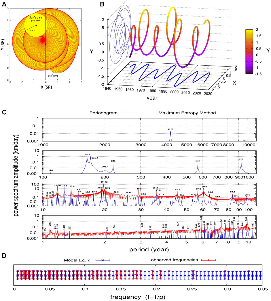
FIGURE 1. (A) The motion the wobbling Sun from 1944 to 2020 (B) The distance and the speed of the Sun relative to the barycenter of the solar system from 1800 to 2020. (C) Periodogram (red) and the maximum entropy method spectrum (blue) of the speed of the Sun from BC 8002-Dec-12, to AD 9001-Apr-24. (D) Comparison between the frequencies observed in (C) in the range 3–200 years (red) and the frequencies predicted by the harmonic model of Eq. 3 (blue). (cf. Scafetta, 2014a).

We can analyze the main orbital frequencies of the planetary system by performing, for example, the harmonic analysis of the solar velocity alone. Its periodograms were obtained with the Fourier analysis (red) and the maximum entropy method (blue) (Press et al., 1997) and are shown in Figure 1C.

Several spectral peaks can be recognized: the ∼1.092 year period of the Earth-Jupiter conjunctions; the ∼9.93 and ∼19.86 year periods of the Jupiter-Saturn spring (half synodic) and synodic cycles, respectively; the ∼11.86, ∼29.5, ∼84 and ∼165 years of the orbital periods of Jupiter, Saturn, Uranus and Neptune, respectively; the ∼60 year cycle of the Trigon of Great Conjunctions between Jupiter and Saturn; the periods corresponding to the synodic cycles between Jupiter and Neptune (∼12.8 year), Jupiter and Uranus (∼13.8 year), Saturn and Neptune (∼35.8 year), Saturn and Uranus (∼45.3) and Uranus and Neptune (∼171.4 year), as well as their spring periods.

The synodic period is defined as

$P_{12}=\frac{1}{f_{12}}={\left|\frac{1}{P_1}-\frac{1}{P_2}\right|}^{-1},(2)$

where P₁ and P₂ are the orbital periods of two planets. Additional spectral peaks at ∼200–220, ∼571, ∼928 and ∼4200 years are also observed. The spring period is the half of P₁₂. The observed orbital periods are listed in Table 1.

TABLE 1

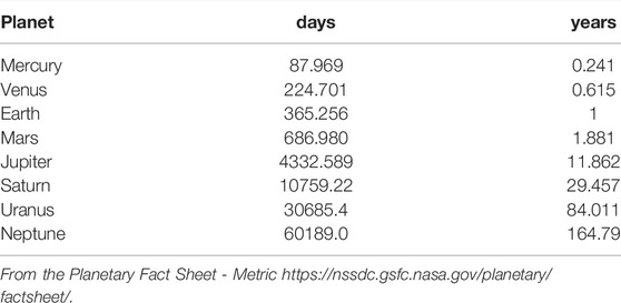
TABLE 1. Sidereal orbital periods of the planets of the solar system.

Some of the prominent frequencies in the power spectra appear clustered around well-known solar cycles such as in the ranges 42–48 years, 54–70 years, 82–100 years (Gleissberg cycle), 155–185 (Jose cycle), and 190–240 years (Suess-de Vries cycle) (e.g.: Ogurtsov et al., 2002; Scafetta and Willson, 2013a). The sub-annual planetary harmonics and their spectral coherence with satellite total solar irradiance records will be discussed in Section 5.

The important result is that the several spectral peaks observed in the solar motion are not randomly distributed but are approximately reproduced using the following simple empirical harmonic formula

$p_i=\frac{178.38}{i}yr,i=\mathrm{1,2,3},\dots ,(3)$

where 178 years corresponds to the period that Jose (1965) found both in the solar orbital motion and in the sunspot records (cf.: Jakubcová and Pick, 1986; Charvátová and Hejda, 2014). A comparison between the observed frequencies and those predicted by the harmonic model of Eq. 3 is shown in Figure 1D, where a strong coincidence is observed. Equation 3 suggests that the solar planetary system is highly self-organized and synchronized.

4 The Schwabe 11-year Solar Cycle

Wolf (1859) himself proposed that the ∼11-year sunspot cycle could be produced by the combined orbital motions of Venus, Earth, Jupiter and Saturn. In the following, we discuss two possible and complementary solar-planetary models made with the orbital periods of these four planets.

4.1 The Venus-Earth-Jupiter Model

The first model relates the 11-year solar cycle with the relative orbital configurations of Venus, Earth and Jupiter, which was first proposed by Bendandi (1931) as recently reminded by Battistini (2011). Later, Bollinger (1952), Hung (2007) and others (e.g.: Scafetta, 2012c; Tattersall, 2013; Wilson, 2013; Stefani et al., 2016, 2019, 2021) developed more evolved models.

This model is justified by the consideration that Venus, Earth and Jupiter are the three major tidal planets (Scafetta, 2012b). Their alignments repeat every:

$\frac{1}{f_{\mathit{V\; EJ}}}=P_{\mathit{V\; EJ}}={\left(\frac{3}{P_V}-\frac{5}{P_E}+\frac{2}{P_J}\right)}^{-1}=22.14yr(4)$

where P_V = 224.701 days, P_E = 365.256 days and P_J = 4332.589 days are the sidereal orbital periods of Venus, Earth and Jupiter, respectively.

The calculated 22.14-year period is very close to the ∼22-year Hale solar magnetic cycle. Since the Earth–Venus–Sun–Jupiter and Sun–Venus–Earth–Jupiter configurations present equivalent tidal potentials, the tidal cycle would have a recurrence of 11.07 years. This period is very close to the average solar cycle length observed since 1750 (Hung, 2007; Scafetta, 2012a; Stefani et al., 2016).

Vos et al. (2004) found evidence for a stable Schwabe cycle with a dominant 11.04-year period over a 10,000-year interval which is very close to the above 11.07 periodicity, as suggested by Stefani et al. (2020a). However, the Jupiter-Saturn model also reproduces a similar Schwabe cycle (see Sections 4.2 and 6).

Equation 4 is an example of “orbital invariant inequality” (Scafetta et al., 2016; Scafetta, 2020). Section 7 explains their mathematical property of being simultaneously and coherently seen by any region of a differentially rotating system like the Sun. This property should favor the synchronization of the internal solar dynamics with external forces varying with those specific frequencies.

Equation 4 can be rewritten in a vectorial formalism as

$\left(3,-\mathrm{5,2}\right)=3\left(1,-\mathrm{1,0}\right)-2\left(\mathrm{0,1},-1\right).(5)$

Each vector can be interpreted a frequency where the order of its components correspond to the arbitrary assumed order of the planets, in this case: (Venus, Earth, Jupiter). Thus, (3, −5, 2) ≡ 3/P_V − 5/P_E + 2/P_J, 3(1, −1, 0) ≡ 3(1/P_V − 1/P_E) and −2(0, 1, −1) ≡ −2(1/P_E − 1/P_J).

We observe that (1, −1, 0) indicates the frequency of the synodic cycle between Venus and Earth and (0, 1, −1) indicates the frequency of the synodic cycle between Earth and Jupiter (Eq. 2). Thus, the vector (3, −5, 2) indicates the frequency of the beat created by the third harmonic of the synodic cycle between Venus and Earth and the second harmonic of the synodic cycle between Earth and Jupiter.

Equation 5 also means that the Schwabe sunspot cycle can be simulated by the function:

$f\left(t\right)=\cos \left(2\pi \cdot 2\cdot 3\frac{t-t_{VE}}{P_{VE}}\right)+\cos \left(2\pi \cdot 2\cdot 2\frac{t-t_{EJ}}{P_{EJ}}\right),(6)$

where t_VE = 2002.8327 is the epoch of a Venus-Earth conjunction whose period is P_VE = 1.59867 years; and t_EJ = 2003.0887 is the epoch of an Earth-Jupiter conjunction whose period is P_EJ = 1.09207 years. The 11.07-year beat is obtained by doubling the synodic frequencies given in Eq. 5.

Figure 2A shows that the three-planet model of Eq. 6 (red) generates a beat pattern of 11.07 years reasonably in phase with the sunspot cycle (blue). More precisely, the maxima of the solar cycles tend to occur when the perturbing forcing produced by the beat is stronger, that is when the spring tides of the planets can interfere constructively somewhere in the solar structure.

FIGURE 2

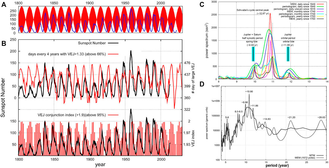
FIGURE 2. (A) The plot of Eq. 6 (red) versus the sunspot numberthe planets can interfere record (blue). (B, Top) The sunspot number record (black) versus the alignment index I_VEJ > 66%. (B, Bottom) The sunspot number record (black) against the number of days of most alignment (I_VEJ > 95%) (red). (C,D) Power spectra of the Schwabe sunspot cycle using the Maximum Entropy Method (MEM) and the periodogram (MTM) (Press et al., 1997). (Data from: https://www.sidc.be/silso/datafiles).

Hung (2007) and Scafetta (2012a) developed the three-planet model by introducing a three-planetary alignment index. In the case of two planets, the alignment index I_ij between planet i and planet j is defined as:

$I_{ij}=|\cos \left({\mathrm{\Theta }}_{ij}\right)|,(7)$

where Θ_ij is the angle between the positions of the two planets relative to the solar center.

Equation 7 indicates that when the two planets are aligned (Θ_ij = 0 or Θ_ij = π), the alignment index has the largest value because these two positions imply a spring-tide configuration. Instead, when Θ_ij = π/2, the index has the lowest value because at right angles–corresponding to a neap-tide configuration–the tides of the two planets tend to cancel each other.

In the case of the Venus-Earth-Jupiter system, there are three correspondent alignment indexes:

$I_V=|\cos \left({\mathrm{\Theta }}_{VE}\right)|+|\cos \left({\mathrm{\Theta }}_{VJ}\right)|(8)$

$I_E=|\cos \left({\mathrm{\Theta }}_{EV}\right)|+|\cos \left({\mathrm{\Theta }}_{EJ}\right)|(9)$

$I_J=|\cos \left({\mathrm{\Theta }}_{JV}\right)|+|\cos \left({\mathrm{\Theta }}_{JE}\right)|.(10)$

Then, the combined alignment index I_VEJ for the three planets could be defined as:

$I_{\mathit{V\; EJ}}=smallestamong\left(I_V,I_E,I_J\right),(11)$

which ranges between 0 and 2.

Figure 2B shows (in red) that the number of the most aligned days of Venus, Earth and Jupiter–estimated by Eq. 11 – presents an 11.07-year cycle. These cycles are well correlated, both in phase and frequency, with the ∼11-year sunspot cycle. Scafetta (2012a) also showed that an 11.08-year recurrence exists also in the amplitude and direction (latitude and longitude components) of the solar jerk-shock vector, which is the time-derivative of the acceleration vector. For additional details see Hung (2007), Scafetta (2012a), Salvador (2013), Wilson (2013) and Tattersall (2013).

A limitation of the Venus-Earth-Jupiter model is that it cannot explain the secular variability of the sunspot cycle which alternates prolonged low and high activity periods such as, for example, the Maunder grand solar minimum between 1645 and 1715, when very few sunspots were observed (cf. Smythe and Eddy, 1977). However, this problem could be solved by the Jupiter-Saturn model (Scafetta, 2012a) discussed below and, in general, by taking into account also the other planets (Scafetta, 2020; Stefani et al., 2021), as discussed in Sections 6 and 7.

The 11.07-year cycle has also been extensively studied by Stefani et al. (2016); Stefani et al. (2018); Stefani et al. (2019, 2020b, 2021) where it is claimed to be the fundamental periodicity synchronizing the solar dynamo.

4.2 The Jupiter-Saturn Model

The second model assumes that the Schwabe sunspot cycle is generated by the combined effects of the planetary motions of Jupiter and Saturn. The two planets generate two main tidal oscillations associated with the orbit of Jupiter (11.86-year period) – which is characterized by a relatively large eccentricity (e = 0.049) – and the spring tidal oscillation generated by Jupiter and Saturn (9.93-year period) (Brown, 1900; Scafetta, 2012c). In this case, the Schwabe sunspot cycle could emerge from the synchronization of the two tides with periods of 9.93 and 11.86 years, whose average is about 11 years.

The Jupiter-Saturn model is supported by a large number of evidences. For example, Scafetta (2012a,b) showed that the sunspot cycle length, i.e. the time between two consecutive sunspot minima, is bi-modally distributed, being always characterized by two peaks at periods smaller and larger than 11 years. This suggests that there are two dynamical attractors at the periods of about 10 and 12 years forcing the sunspot cycle length to fall either between 10 and 11 years or between 11 and 12 years. Sunspot cycles with a length very close to 11 years are actually absent. In addition, Figures 2C,D show the periodograms of the monthly sunspot record since 1749. The spectral analysis of this long record reveals the presence of a broad major peak at about 10.87 years obtained by some solar dynamo models (Macario-Rojas et al., 2018) which is surrounded by two minor peaks at 9.93 and 11.86 years that exactly correspond with the two main tides of the Jupiter-Saturn system.

In Section 6 we will show that the combination of these three harmonics produces a multidecadal, secular and millennial variability that is rather well correlated with the long time-scale solar variability.

5 Solar Cycles Shorter Than the Schwabe 11-year Solar Cycle

On small time scales, Bigg (1967) found an influence of Mercury on sunspots. Indeed, in addition to Jupiter, Mercury can also induce relatively large tidal cycles on the Sun because its orbit has a large eccentricity (e = 0.206) (Scafetta et al. 2019a).

Rapid oscillations in the solar activity can be optimally studied using the satellite total solar irradiance (TSI) records. Since 1978, TSI data and their composites have been obtained by three main independent science teams: ACRIMSAT/ACRIM3 (Willson and Mordvinov, 2003), SOHO/VIRGO (Fröhlich, 2006) and SORCE/TIM (Kopp and Lawrence, 2005a; Kopp et al., 2005b). Figure 3 compares the ACRIM3, VIRGO and TIM TSI from 2000 to 2014; the average irradiance is about 1361 W/m².

FIGURE 3

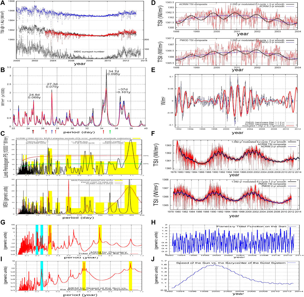
FIGURE 3. (A) Comparison of ACRIMSAT/ACRIM3 (black), SOHO/VIRGO (blue) and SORCE/TIM (red) TSI records versus daily sunspot number (gray). (B) Power spectrum comparison of ACRIMSAT/ACRIM3 (black), SOHO/VIRGO (blue) and SORCE/TIM (red) TSI from 2003.15 to 2011.00. The arrows at the bottom depicts the periods reported in Table 2. (C, Top) Periodogram of ACRIM results in W²/m⁴ from 1992.5–2012. (C, Bottom) Power spectra of ACRIM from 1992.5 to 2012.9) and of PMOD from 1997.75 to 2004.25. The yellow bars schematically indicate the harmonics generated by the planets as reported in Tables 2–4. (D) ACRIM and PMOD TSI composites during solar maximum 23 (1998–2004). The black curve is from Eqs 7, 8. (E) High-pass filter of the PMOD (blue) and ACRIM (black) TSI compared against a 1.092-year harmonic Jupiter function (red). (F) ACRIM and PMOD TSI since 1978 (red) against the models of Eqs 13, 14. (G,H) Planetary tidal function on the Sun (blue) (see Figure 8C) and its power spectrum (red). (I, J) Speed of the Sun relative to the solar system barycenter (blue) and its power spectrum (red). (cf. Scafetta and Willson, 2013b,c).

5.1 The 22–40 days Time-Scale

Figure 3B shows the power spectra in the 22–40 days range of the three TSI records (Figure 3A) from 2003.15 to 2011.00 (Scafetta and Willson, 2013c). A strong spectral peak is observed at ∼27.3 days (0.075 years) (Willson and Mordvinov, 1999), which corresponds to the synodic period between the Carrington solar rotation period of ∼25.38 days and the Earth’s orbital period of ∼365.25 days. The Carrington period refers to the rotation of the Sun at 26° of latitude, where most sunspots form and the solar magnetic activity emerges (Bartels, 1934). The observed 27.3-day period differs from the Carrington 25.38-day period because the Sun is seen from the orbiting Earth. Thus, the 27.3-day period derives from Eq. 2 using T₁ = 25.38 days and T₂ = 365.25 days.

Figure 3B reveals additional spectral peaks at $\sim 24.8$ days ($\sim 0.068$ years), $\sim 34$-35 days ($\sim 0.093$-0.096 years), and $\sim 36$-38 days ($\sim 0.099$-0.104 years). They fall within the range of the solar differential rotation that varies from 24.7–25.4 days near the equator (Kotov, 2020) to about 38 days near the poles (Beck, 2000).

However, the same periods appear to be also associated with the motion of the planets. In fact, the $\sim 24.8$-day cycle corresponds to the synodic period between the sidereal orbital period of Jupiter ($\sim 4332.6$ days) and the sidereal equatorial rotation period of the Sun ($\sim 24.7$ days) calculated using Eq. 2. Additional synodic cycles between the rotating solar equator and the orbital motion of the terrestrial planets are calculated at $\sim 26.5$ days, relative to the Earth, $\sim 27.75$ days, relative to Venus, and $\sim 34.3$ days, relative to Mercury (see Table 2). We also notice that the major TSI spectral peak at 34.7 days is very close to the $\sim 34.3$-day Mercury-Sun synodic period, although it would require the slightly different solar rotation period of 24.89 days.

TABLE 2

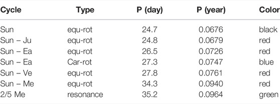
TABLE 2. Solar equatorial (equ) and Carrington (Car) rotation cycles relative to the fixed stars and to the four major tidally active planets calculated using Eq. 2 where P₁ = 24.7 days is the sidereal equatorial solar rotation and P₂ the orbital period of a planet. Last column: color of the arrows in Figure 3B (cf. Scafetta and Willson, 2013c).

5.2 The 0.1–1.1 year Time-Scale

Tables 3, 4 collect the orbital periods, the synodic cycles and their harmonics among the terrestrial planets (Mercury, Venus, Earth and Mars). The tables also show the synodic cycles between the terrestrial and the Jovian planets (Jupiter, Saturn, Uranus, and Neptune). The calculated periods are numerous and clustered. If solar activity is modulated by planetary motions, these frequency clusters should be observed also in the TSI records.

TABLE 3

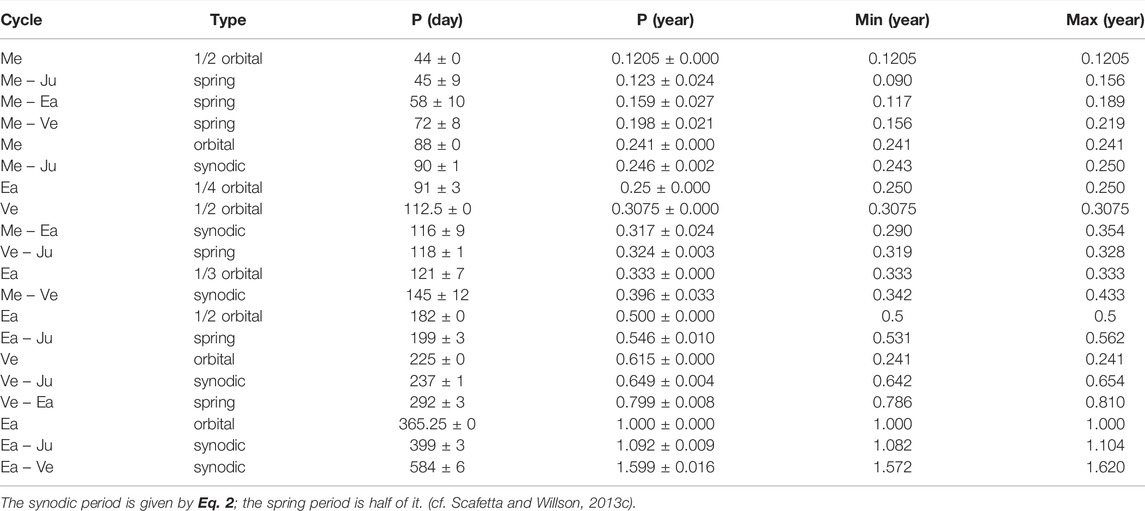
TABLE 3. Major theoretical planetary harmonics with period p < 1.6 years.

TABLE 4

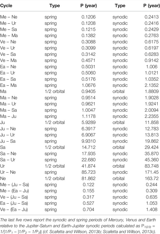
TABLE 4. Additional expected harmonics associated with planetary orbits.

Figure 3C shows two alternative power spectra of the ACRIM and PMOD TSI records superposed to the distribution (yellow) of the planetary frequencies reported in Tables 2–4. The main power spectral peaks are observed at: $\sim 0.070$, $\sim 0.097$, $\sim 0.20$, $\sim 0.25$, 0.30–0.34, $\sim 0.39$, $\sim 0.55$, 0.60–0.65, 0.7–0.9, and 1.0–1.2 years.

Figure 3C shows that all the main spectral peaks observed in the TSI records appear compatible with the clusters of the calculated orbital harmonics. For example: the Mercury-Venus spring-tidal cycle (0.20 years); the Mercury orbital cycle (0.24 years); the Venus-Jupiter spring-tidal cycle (0.32 years); the Venus-Mercury synodic cycle (0.40 years); the Venus-Jupiter synodic cycle (0.65 years); and the Venus-Earth spring tidal cycle (0.80 years). A 0.5-year cycle is also observed, which could be due to the Earth crossing the solar equatorial plane twice a year and to a latitudinal dependency of the solar luminosity. These results are also confirmed by the power spectra of the planetary tidal function on the Sun (see Figure 8C) and of the speed of the Sun relative to the solar system barycenter (Figures 3G-J).

The 1.0–1.2 year band observed in the TSI records correlates well with the 1.092-year Earth-Jupiter synodic cycle. Actually, the TSI records present maxima in the proximity of the Earth-Jupiter conjunction epochs (Scafetta and Willson, 2013b).

Figure 3D shows the ACRIM and PMOD TSI records (red curves) plotted against the Earth-Jupiter conjunction cycles with the period of 1.092 years (black curve) from 1998 to 2004. TSI peaks are observed around the times of the conjunctions. The largest peak occurs at the beginning of 2002 when the conjunction occurred at a minimum of the angular separation between Earth and Jupiter (0°13’ 19”).

Figure 3E shows the PMOD (blue) and ACRIM (black) records band-pass filtered to highlight the 1.0–1.2 year modulation. The two curves (blue and black) are compared to the 1.092-year harmonic function (red):

$f\left(t\right)=g\left(t\right)\cos \left[2\pi \frac{\left(t-2002\right)}{1.09208}\right],(12)$

where the amplitude g(t) was modulated according to the observed Schwabe solar cycle. The time-phase of the oscillation is chosen at t_EJ = 2002 because one of the Earth-Jupiter conjunctions occurred on the 1^st of January 2002. The average Earth-Jupiter synodic period is 1.09208 years. The TSI 1.0–1.2 year oscillation is significantly attenuated during solar minima (1995–1997 and 2007–2009) and increases during solar maxima. In particular, the figure shows the maximum of solar cycle 23 and part of the maxima of cycles 22 and 24 and confirms that the TSI modulation is well correlated with the 1.092-year Earth-Jupiter conjunction cycle.

Figure 3F extends the model prediction back to 1978. Here the TSI records are empirically compared against the following equations: for ACRIM,

$f\left(t\right)=S_A\left(t\right)+0.2\left(S_A\left(t\right)-1360.58\right)\cos \left[2\pi \frac{\left(t-2002\right)}{1.09208}\right];(13)$

for PMOD,

$f\left(t\right)=S_P\left(t\right)+0.2\left(S_P\left(t\right)-1365.3\right)\cos \left[2\pi \frac{\left(t-2002\right)}{1.09208}\right].(14)$

The blue curves are the 2-year moving averages, S_A(t) and S_P(t), of the ACRIM and PMOD TSI composite records, respectively. The data-model comparison confirms that the 1.092-year Earth-Jupiter conjunction cycle is present since 1978. In fact, TSI peaks are also found in coincidences with a number of Earth-Jupiter conjunction epochs like those of 1979, 1981, 1984, 1990, 1991, 1992, 1993, 1994, 1995, 1998, 2011 and 2012. The 1979 and 1990 peaks are less evident in the PMOD TSI record, likely because of the significant modifications of the published Nimbus7/ERB TSI record in 1979 and 1989–1990 proposed by the PMOD science team (Fröhlich, 2006; Scafetta, 2009; Scafetta et al., 2011).

The result suggests that the side of the Sun facing Jupiter could be slightly brighter, in particular during solar maxima. Thus, when the Earth crosses the Sun-Jupiter line, it could receive an enhanced amount of radiation. This coalesces with strong hotspots observed on other stars with orbiting close giant planets (Shkolnik et al., 2003, 2005). Moreover, Kotov and Haneychuk (2020) analyzed 45 years of observations and showed that the solar photosphere, as seen from the Earth, is pulsating with two fast and relatively stable periods P₀ = 9600.606(12) s and P₁ = 9597.924(13) s. Their beatings occur with a period of 397.7(2.6) days, which coincides well with the synodic period between Earth and Jupiter (398.9 days). A hypothesis was advanced that the gravity field of Jupiter could be involved in the process.

5.3 The Solar Cycles in the 2–9 years Range

The power spectrum in Figure 2D shows peaks at 5-6 and 8.0–8.5 years. The former ones appear to be harmonics of the Schwabe 11-year solar cycle discussed in Section 3. The latter peaks are more difficult to be identified. In any case, some planetary harmonics involving Mercury, Venus, Earth, Jupiter and Saturn could explain them.

For example, the Mercury-Venus orbital combination repeats almost every 11.08 years, which is similar to the 11.07-year invariant inequality between Venus, Earth and Jupiter discussed in Section 3. In fact, P_M = 0.241 years and P_V = 0.615 years, therefore their closest geometrical recurrences occur after 23 orbits of Mercury (23P_M = 5.542 years) and nine orbits of Venus (9P_V = 5.535 year). Moreover, we have 46P_M = 11.086 years and 18P_V = 11.07 years. Thus, the orbital configuration of Mercury and Venus repeats every 5.54 years as well as every 11.08 years and might contribute to explain the 5–6 years spectral peak observed in Figure 2D. Moreover, eight orbits of the Earth (8P_E = 8 years) and 13 orbits of Venus (13P_V = 7.995 years) nearly coincide and this combination might have contributed to produce the spectral peak at about 8 years.

There is also the possibility that the harmonics at about 5.5 and 8–9 years could emerge from the orbital combinations of Venus, Earth, Jupiter and Saturn. In fact, we have the following orbital invariant inequalities

${\left(\frac{2}{P_V}-\frac{3}{P_E}-\frac{2}{P_J}+\frac{3}{P_S}\right)}^{-1}=5.43year(15)$

and

$2{\left(-\frac{1}{P_V}+\frac{2}{P_E}-\frac{2}{P_J}+\frac{1}{P_S}\right)}^{-1}=8.34year,(16)$

where the orbital periods of the four planets are given in Table 1. Equation 15 combines the spring cycle between Venus and Jupiter with the third harmonic of the synodic cycle between Earth and Saturn. Equation 16 is the first inferior harmonic (because of the factor 2) of a combination of the synodic cycle between Venus and Saturn and the spring cycle between Earth and Jupiter. Eqs 15, 16 express orbital invariant inequalities, whose general physical properties are discussed in Section 7.

The above results, together with those discussed in Section 4, once again suggest that the major features of solar variability at the decadal scale from 2 to 22 years could have been mostly determined by the combined effect of Venus, Earth, Jupiter and Saturn, as it was first speculated by Wolf (1859).

6 The Multi-Decadal and Millennial Solar Cycles Predicted by the Jupiter-Saturn Model

As discussed in Section 4.1, the Jupiter-Saturn model interprets quite well two of the three main periods that characterize the sunspot number record since 1749: P_S1 = 9.93, P_S2 = 10.87 and P_S3 = 11.86 years (Figure 2C) (Scafetta, 2012a). The two side frequencies match the spring tidal period of Jupiter and Saturn (9.93 years), and the tidal sidereal period of Jupiter (11.86 years). The central peak at P_S2 = 10.87 years can be associated with a possible natural dynamo frequency that is also predicted by a flux-transport dynamo model (Macario-Rojas et al., 2018). However, the same periodicity could be also interpreted as twice the invariant inequality period of Eq. 15, which gives 10.86 years. According to the latter interpretation, the central frequency sunspot peak might derive from a dynamo synchronized by a combination of the orbital motions of Venus, Earth, Jupiter and Saturn.

The three harmonics of the Schwabe frequency band beat at P_S13 = 60.95 years, P_S12 = 114.78 years and P_S23 = 129.95 years. Using the same vectorial formalism introduced in Section 3.1 to indicate combinations of synodical cycles, a millennial cycle, P_S123, is generated by the beat between P_S12 ≡ (1, −1, 0) and P_S23 ≡ (0, 1, −1) according to equation (1, −1, 0) − (0, 1, −1) = (1, −2, 1) that corresponds to the period

$P_{\mathit{S123}}={\left(\frac{1}{P_{S1}}-\frac{2}{P_{S2}}+\frac{1}{P_{S3}}\right)}^{-1}\approx 983year,(17)$

where we adopted the multi-digits accurate values P_S1 = 9.929656 years, P_S2 = 10.87 years and P_S3 = 11.862242 years (Table 1). However, the millennial beat is very sensitive to the choice of P_S2.

To test whether this three-frequency model actually fits solar data, Scafetta (2012a) constructed its constituent harmonic functions by setting their relative amplitudes proportional to the power of the spectral peaks of the sunspot periodogram. The three amplitudes, normalized with respect to A_S2, are: A_S1 = 0.83, A_S2 = 1, A_S3 = 0.55.

The time-phases of the two side harmonics are referred to: t_S1 = 2000.475, which is the synodic conjunction epoch of Jupiter and Saturn (23/June/2000) relative to the Sun, when the spring tide must be stronger; and t_S3 = 1999.381, which is the perihelion date of Jupiter (20/May/1999) when its tide is stronger. The time-phase of the central harmonic was set to t_S2 = 2002.364 and was estimated by fitting the sunspot number record with the three-harmonic model keeping the other parameters fixed.

The time-phases of the beat functions are calculated using the equation

$t_{12}=\frac{P_2{t}_1-P_1{t}_2}{P_2-P_1}.(18)$

It was found t_S12 = 2095.311, t_S13 = 2067.044 and t_S23 = 2035.043. The time-phase of the beat between P_S12 and P_S23 was calculated as t_S123 = 2059.686. Herein, we ignore that the phases for the conjunction of Jupiter and Saturn vary by a few months from the average because the orbits are elliptic, which could imply a variation up to a few years of the time-phases of the beat functions.

The proposed three-frequency harmonic model is then given by the function

$\sum _{i=1}^3{h}_i\left(t\right)=\sum _{i=1}^3{A}_{Si}\cos \left(2\pi \frac{t-t_{Si}}{P_{Si}}\right).(19)$

The components and the beat functions generated by the model are given by the equations

$h_1\left(t\right)=0.83\cos \left(2\pi \frac{t-2000.475}{9.929656}\right),(20)$

$h_2\left(t\right)=1.0\cos \left(2\pi \frac{t-2002.364}{10.87}\right),(21)$

$h_3\left(t\right)=0.55\cos \left(2\pi \frac{t-1999.381}{11.862242}\right).(22)$

Thus, the final model becomes

$h_{123}\left(t\right)=h_1\left(t\right)+h_2\left(t\right)+h_3\left(t\right).(23)$

To emphasize its beats we can also write

$f_{123}\left(t\right)=\left\{\begin{array}{cc}{h}_{123}\left(t\right)\hfill & \text{if\hspace{0.17em}}{h}_{123}\left(t\right)\ge 0\hfill \\ 0\hfill & \text{if\hspace{0.17em}}{h}_{123}\left(t\right)<0\hfill \end{array}\right.(24)$

The resulting envelope functions of the beats are

$b_{12}\left(t\right)=0.60\cos \left(2\pi \frac{t-1980.528}{114.783}\right)(25)$

$b_{13}\left(t\right)=0.40\cos \left(2\pi \frac{t-2067.044}{60.9484}\right)(26)$

$b_{23}\left(t\right)=0.45\cos \left(2\pi \frac{t-2035.043}{129.951}\right)(27)$

Figure 4 shows the three-frequency solar model of Eq. 24 (red). Figure 4A compares it against two reconstructions of the solar activity based on ¹⁰Be and ¹⁴C cosmogenic isotopes (blue and black, respectively) (Bard et al., 2000; Steinhilber et al., 2009). The millennial beat cycle is represented by the green curve. The model correctly hindcast all solar multi-decadal grand minima observed during the last 1000 years, known as the Oort, Wolf, Spörer, Maunder and Dalton grand solar minima. They approximately occurred when the three harmonics interfered destructively. Instead, the multi-decadal grand maxima occurred when the three harmonics interfere constructively generating a larger perturbation on the Sun.

FIGURE 4

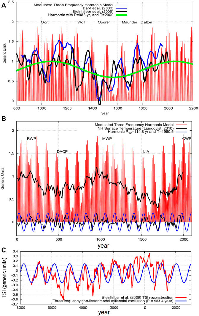
FIGURE 4. (A) Eq. 40 (red) against two reconstructions of solar activity based on ¹⁰Be and ¹⁴C cosmogenic isotopes (Bard et al., 2000; Steinhilber et al., 2009). (B). Equation 40 (red) against a Northern Hemisphere proxy temperature reconstruction by Ljungqvist (2010). (C) The millennial oscillation predicted by the three-frequency non-linear solar model (blue) versus the TSI proxy model by Steinhilber et al. (2009) (red). (cf. Scafetta, 2012a; 2014b).

Figure 4B compares Eq. 24 against the Northern Hemisphere proxy temperature reconstruction of Ljungqvist (2010) (black). We notice the good time-matching between the oscillations of the model and the temperature record of both the millennial and the 115-year modulations, which is better highlighted by the smoothed filtered curves at the bottom of the figure. The Roman Warm Period (RWP), Dark Age Cold Period (DACP), Medieval Warm Period (MWP), Little Ice Age (LIA) and the Current Warm Period (CWP) are well hindcast by the three-frequency Jupiter-Saturn model.

Figure 4C shows the millennial oscillation (blue) predicted by Eq. 24 given by

$g_m\left(t\right)=\cos \left(2\pi \frac{t-2059.686}{983.401}\right).(28)$

The curve is well correlated with the quasi millennial solar oscillation–known as the Eddy oscillation–throughout the Holocene as revealed by the ¹⁴C cosmogenic isotope record (red) and other geological records (Kerr, 2001; Steinhilber et al., 2009; Scafetta, 2012a, 2014b).

Scafetta (2012a) discussed other properties of the three-frequency solar model. For example, five 59–63 year cycles appear in the period 1850–2150, which are also well correlated with the global surface temperature maxima around about 1880, 1940 and 2000. The model also predicts a grand solar minimum around the 2030s constrained between two grand solar maxima around 2000 and 2060. The modeled solar minimum around 1970, the maximum around 2000 and the following solar activity decrease, which is predicted to last until the 2030s, are compatible with the multidecadal trends of the ACRIM TSI record (Willson and Mordvinov, 2003), but not with those shown by the PMOD one (Fröhlich, 2006) that uses TSI modified data (Scafetta et al., 2019b) and has a continuous TSI decrease since 1980. The plots of ACRIM and PMOD TSI data are shown in Figure 3F and have been extensively commented by Scafetta et al. (2019b). Finally, the model also reproduces a rather long Schwabe solar cycle of about 15 years between 1680 and 1700. This long cycle was actually observed both in the δ¹⁸O isotopic concentrations found in Japanese tree rings (a proxy for temperature changes) and in ¹⁴C records (a proxy for solar activity) (Yamaguchia et al., 2010).

Scafetta (2014b) also suggested that the input of the planetary forcing could be nonlinearly processed by the internal solar dynamo mechanisms. As a consequence, the output function might be characterized by additional multi-decadal and secular harmonics. The main two frequency clusters are predicted at 57, 61, 65 years and at 103, 115, 130, and 150 years. These harmonics actually appear in the power spectra of solar activity (Ogurtsov et al., 2002). In particular, Cauquoin et al. (2014) found the four secular periods (103, 115, 130, 150 years) in the ¹⁰Be record of 325–336 kyr ago. These authors claimed that their analyzed records do not show any evidence of a planetary influence but they did not realize that their found oscillations could be derived from the beating among the harmonics of Jupiter and Saturn with the 11-year solar cycle, as demonstrated in Scafetta (2014b).

We notice that the multi-secular and millennial hindcasts of the solar activity records made by the three-frequency Jupiter-Saturn model shown in Figure 4 are impressive because the frequencies, phases and amplitudes of the model are theoretically deduced from the orbits of Jupiter and Saturn and empirically obtained from the sunspot record from 1750 to 2010. The prolonged periods of high and low solar activity derive from the constructive and destructive interference of the three harmonics.

7 Orbital Invariant Inequality Model: The Jovian Planets and the Long Solar and Climatic Cycles

The orbital invariant inequality model was first proposed by Scafetta et al. (2016) and successively developed by Scafetta (2020) using only the orbital periods of the four Jovian planets (Table 1). It successfully reconstructs the main solar multi-decadal to millennial oscillations like those observed at 55–65 years, 80–100 years (Gleissberg cycle), 155–185 years (Jose cycle), 190–240 years (Suess - de Vries cycle), 800–1200 years (Eddy cycle) and at 2100–2500 years (Bray-Hallstatt cycle) (McCracken et al., 2001, 2013; Abreu et al., 2012; Scafetta, 2016). The model predictions well agree with the solar and climate long-term oscillations discussed, for example, in Neff et al. (2001) and McCracken et al. (2013). Let us now describe the invariant inequality model in some detail.

Given two harmonics with period P₁ and P₂ and two integers n₁ and n₂, there is a resonance if P₁/P₂ = n₁/n₂. In the real planetary motions, this identity is almost always not satisfied. Consequently, it is possible to define a new frequency f and period P using the following equation

$f=\frac{1}{P}=\left|\frac{n_1}{P_1}-\frac{n_2}{P_2}\right|,(29)$

which is called “inequality.” Clearly, f and P represent the beat frequency and the beat period between n₁/P₁ and n₂/P₂. The simplest case is when n₁ = n₂ = 1, which corresponds to the synodal period between two planets defined in Eq. 2, which is reported below for convenience:

$P_{12}=\frac{1}{f_{12}}={\left|\frac{1}{P_1}-\frac{1}{P_2}\right|}^{-1}.(30)$

Equation 30 indicates the average time interval between two consecutive planetary conjunctions relative to the Sun. The conjunction periods among the four Jovian planets are reported in Table 5.

TABLE 5

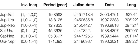
TABLE 5. Heliocentric synodic invariant inequalities and periods with the timing of the planetary conjunctions closest to 2000 AD (cf. Scafetta, 2020).

Equation 29 can be further generalized for a system of n orbiting bodies with periods P_i (i = 1, 2, …, n). This defines a generic inequality, represented by the vector (a₁, a₂, …, a_n), as

$f=\frac{1}{P}=\left|\sum _{i=1}^n\frac{a_i}{P_i}\right|,(31)$

where a_i are positive or negative integers.

Among all the possible orbital inequalities given by Eq. 31, there exists a small subset of them that is characterized by the condition:

$\sum _{i=1}^n{a}_i=0.(32)$

This special subset of frequencies is made of the synodal planetary periods (Eq. 30) and all the beats among them.

It is easy to verify that the condition imposed by Eq. 32 has a very important physical meaning: it defines a set of harmonics that are invariant with respect to any rotating system such as the Sun and the heliosphere. Given a reference system at the center of the Sun and rotating with period P_o, the orbital periods, or frequencies, seen relative to it are given by

$f_i^{\prime }=\frac{1}{P_i^{\prime }}=\frac{1}{P_i}-\frac{1}{P_o}.(33)$

With respect to this rotating frame of reference, the orbital inequalities among more planets are given by:

$f^{\prime }=\frac{1}{P^{\prime }}=\left|\sum _{i=1}^n\frac{a_i}{P_i^{\prime }}\right|=\left|\sum _{i=1}^n\frac{a_i}{P_i}-\frac{{\sum }_{i=1}^n{a}_i}{P_o}\right|.(34)$

If the condition of Eq. 32 is imposed, we have that f′ = f and P′ = P. Therefore, this specific set of orbital inequalities remains invariant regardless of the rotating frame of reference from which they are observed.

For example, the conjunction of two planets relative to the Sun is an event that is observed in the same way in all rotating systems centered in the Sun. Since the Sun is characterized by a differential rotation that depends on its latitude, this means that all solar regions simultaneously feel the same planetary beats, which can strongly favor the emergence of synchronized phenomena in the Sun. Due to this physical property, the orbital inequalities that fulfill the condition given by Eq. 32 were labeled as “invariant” inequalities.

Table 6 reports the orbital invariant inequalities generated by the large planets (Jupiter, Saturn, Uranus, and Neptune) up to some specific order. They are listed using the vectorial formalism:

$f=\frac{1}{P}=\left(a_1,a_2,a_3,a_4\right),(35)$

where a₁ (for Jupiter), a₂ (for Saturn), a₃ (for Uranus) and a₄ (for Neptune) are positive or negative integers and their sum is zero (Eq. 32).

TABLE 6

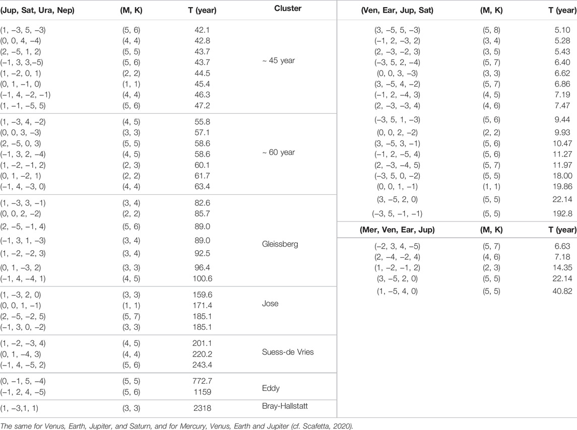
TABLE 6. (Left) List of invariant inequalities for periods T ≥ 40 years and M ≤ 5 for Jupiter, Saturn, Uranus, Neptune (Right).

Two order indices, M and K, can also be used. M is the maximum value among |a_i| and K is defined as

$K=\frac{1}{2}\left(|a_1|+|a_2|+|a_3|+|a_4|\right).(36)$

Since for the invariant inequalities the condition of Eq. 32 must hold, K indicates the number of synodal frequencies between Jovian planet pairs producing a specific orbital invariant. For example, K = 1 means that the invariant inequality is made of only one synodal frequency between two planets, K = 2 indicates that the invariant inequality is made of two synodal frequencies, etc.

For example, the invariant inequality cycle (1, −3, 1, 1) has K = 3 and it is the beat obtained by combining the synodal cycles of Jupiter-Saturn, Saturn-Uranus and Saturn-Neptune because it can be decomposed into three synodal cycles like (1, −3, 1, 1) = (1, −1, 0, 0) − (0, 1, −1, 0) − (0, 1, 0, −1). In the same way, it is possible to decompose any other orbital invariant inequality. Hence, all the beats among the synodal cycles are invariant inequalities and can all be obtained using the periods and time-phases listed in Table 5.

Table 6 lists all the invariant inequalities of the four Jovian planets up to M = 5. They can be collected into clusters or groups that recall the observed solar oscillations. The same frequencies are also shown in Figures 5A,B revealing a harmonic series characterized by clusters with a base frequency of 0.00558 1/year that corresponds to the period of 179.2 years, which is known as the Jose cycle (1965) (Fairbridge and Shirley, 1987; Landscheidt, 1999).

FIGURE 5

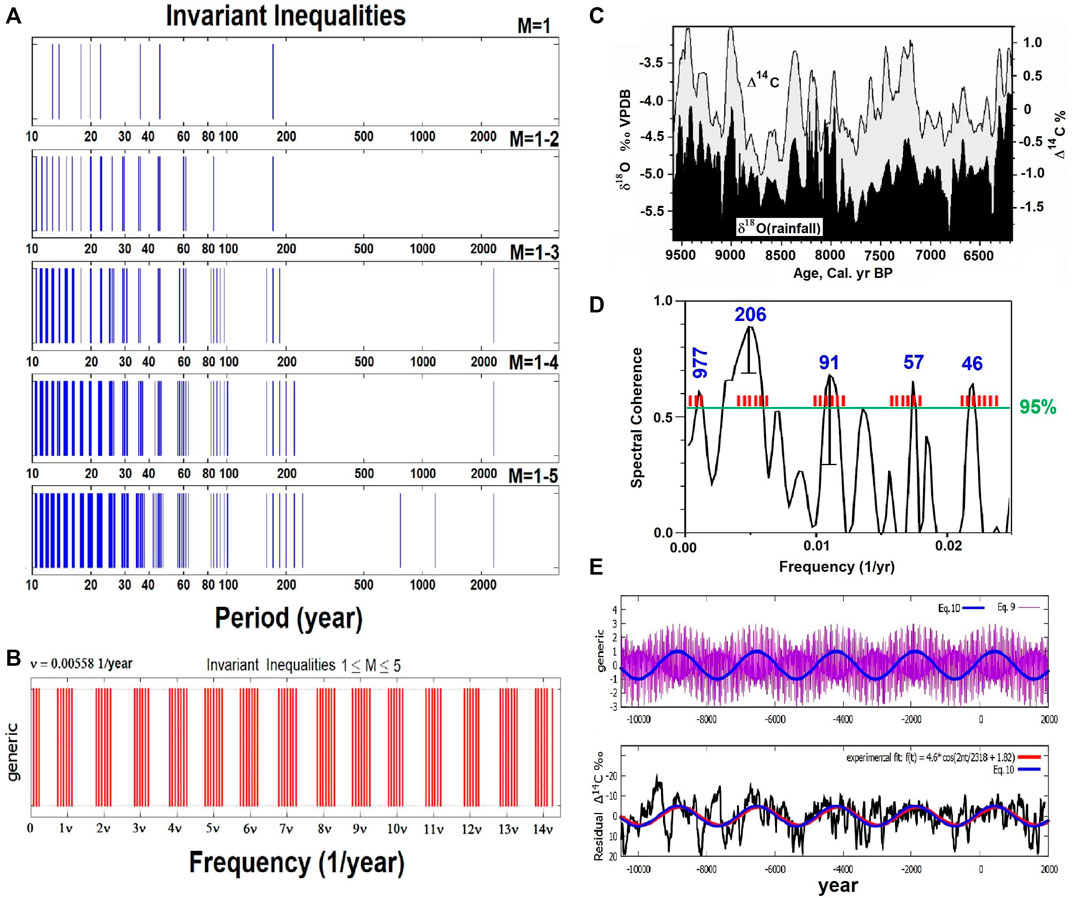
FIGURE 5. (A) The periods of the orbital invariant inequalities produced by Jupiter, Saturn, Uranus and Neptune for 1 ≤ M ≤ 5. (B) The same harmonics highlighting their base frequency ν of the Jose cycle (179.2 years). (cf. Scafetta, 2020). (C) Visual correlation between the INTCAL98 atmospheric Δ¹⁴C record (Stuiver et al., 1998) and a speleothem calcite δ¹⁸O record (adapted from Neff et al., 2001). (D) Comparison between the cross-spectral analysis of the two records in C against the invariant inequalities of the solar system of Table 6 (red bars). (cf. Scafetta, 2020). (E, Top) Eqs 39, 40 that model the Hallstatt oscillation predicted by the invariant inequality (1, −3, 1, 1). (E, Bottom) Eq. 40 (blue) against the Δ¹⁴C record (black) throughout the Holocene (Reimer et al., 2004, IntCal04.14c) and the observed Hallstatt oscillation deduced from a regression harmonic model (red). (cf. Scafetta et al., 2016; Scafetta, 2020).

The physical importance of the harmonics listed in Table 6 is shown in Figure 5C, which compares a solar activity reconstruction from a ¹⁴C record, and the climatic reconstruction from a δ¹⁸O record covering the period from 9500 to 6000 years ago (Neff et al., 2001): the two records are strongly correlated.

Figure 5D shows that the two records present numerous common frequencies that correspond to the cycles of Eddy (800–1200 years), Suess-de Vries (190–240 years), Jose (155–185 years), Gleissberg (80–100 years), the 55–65 year cluster, another cluster at 40–50 years, and some other features. Figure 5D also compares the common spectral peaks of the two records against the clusters of the invariant orbital inequalities (red bars) reported in Figure 5B and listed in Table 6. The figure shows that the orbital invariant inequality model well predicts all the principal frequencies observed in solar and climatic data throughout the Holocene.

The efficiency of the model in hindcasting both the frequencies and the phases of the observed solar cycles can also be more explicitly shown. For example, the model perfectly predicts the great Bray-Hallstatt cycle (2100–2500 years) that was studied in detail by McCracken et al. (2013) and Scafetta et al. (2016). The first step to apply the model is to determine the constituent harmonics of the invariant inequality (1, −3, 1, 1). This cycle is a combination of the orbital periods of Jupiter, Saturn, Uranus and Neptune that gives

$P_{\mathit{JSUN}}=\frac{1}{f_{\mathit{JSUN}}}={\left(\frac{1}{P_j}-\frac{3}{P_S}+\frac{1}{P_U}+\frac{1}{P_N}\right)}^{-1}=2317.56yr.(37)$

The constituent harmonics are the synodic cycles of Jupiter-Saturn, Saturn-Uranus and Saturn-Neptune as described by the following relation

$\left(1,-\mathrm{3,1,1}\right)=\left(1,-\mathrm{1,0,0}\right)-\left(\mathrm{0,1},-\mathrm{1,0}\right)-\left(\mathrm{0,1,0},-1\right).(38)$

Thus, the invariant inequality (1, −3, 1, 1) is the longest beat modulation generated by the superposition of these three synodic cycles and it can be expressed as the periodic function

$f\left(t\right)=\sin \left(2\pi \frac{t-t_{JS}}{P_{JS}}\right)+\sin \left(2\pi \frac{t-t_{SU}}{P_{SU}}\right)+\sin \left(2\pi \frac{t-t_{SN}}{P_{SN}}\right)(39)$

where P_ij are the synodic periods and t_ij are the correspondent time-phases listed in Table 5.

Equation 39 is plotted in Figure 5E and shows the long beat modulation superposed to the Bray-Hallstatt period of 2318 years found in the Δ¹⁴C (‰) record (black) throughout the Holocene (Reimer et al., 2004, IntCal04.14c). This beat cycle is captured, for example, by the function:

$f_B\left(t\right)=-\sin \left(2\pi \frac{t-t_{JS}}{P_{JS}}-2\pi \frac{t-t_{SU}}{P_{SU}}-2\pi \frac{t-t_{SN}}{P_{SN}}\right),(40)$

whose period is 2318 years and the timing is fixed by the three conjunction epochs and the respective synodic periods. In fact, the argument of the above sinusoidal function is the sum of three terms that correspond to those of Eq. 38. Equation 40 is plotted in Figure 5E as the blue curve.

Three important invariant inequalities – (1, −3, 2, 0), (0, 0, 1, −1) and (−1, 3, 0, −2) – are found within the Jose 155–185 year period band:

$P_{\mathit{JSU}}=\frac{1}{f_{\mathit{JSU}}}={\left(\frac{1}{P_J}-\frac{3}{P_S}+\frac{2}{P_U}\right)}^{-1}=159.59yr,(41)$

$P_{UN}=\frac{1}{f_{UN}}={\left(\frac{1}{P_U}-\frac{1}{P_N}\right)}^{-1}=171.39yr,(42)$

$P_{\mathit{JSN}}=\frac{1}{f_{\mathit{JSN}}}={\left(-\frac{1}{P_J}+\frac{3}{P_S}-\frac{2}{P_N}\right)}^{-1}=185.08yr.(43)$

The long beat between Eq. 42 and Eq. 41 – that is (0, 0, 1, −1) − (−1, 3, 0, −2) = (1, −3, 1, −1) – is the great Bray–Hallstatt cycle. The fast beat between Eq. 42 and Eq. 43 – (0, 0, 1, −1) + (−1, 3, 0, −2) = (−1, 3, 1, −3) – is the Gleissberg 89-year cycle, which also corresponds to half of the Jose period of ∼178 year that regulates the harmonic structure of the wobbling of the solar motion.

Another interesting invariant inequality is (1, −2, −1, 2) = (1, 0, −1, 0) − 2(0, 1, 0, −1), which is a beat between the synodic period of Jupiter and Uranus (1,0,-1,0) and the first harmonic of the synodic period of Saturn and Neptune. The period is:

$P_{\mathit{JSN}}=\frac{1}{f_{\mathit{JSN}}}={\left(\frac{1}{P_J}-\frac{2}{P_S}-\frac{1}{P_U}+\frac{2}{P_N}\right)}^{-1}=60.1yr,(44)$

The beat oscillation is given by the equation:

$f\left(t\right)=\cos \left(2\pi \frac{t-t_{JU}}{P_{JU}}\right)+\cos \left(2\pi \cdot 2\frac{t-t_{SN}}{P_{SN}}\right),(45)$

that shows a 60.1-year beat oscillation. The pattern is found in both solar and climate records and could be physically relevant because the maxima of the 60-year beat occur during specific periods–the 1880s, 1940s, and 2000s–that were characterized by maxima in climatic records of global surface temperatures and in other climate records (Agnihotri and Dutta, 2003; Scafetta, 2013, 2014c; Wyatt and Curry, 2014). The 60-year oscillation was even found in the records of the historical meteorite falls in China from AD 619–1943 (Chang and Yu, 1981; Yu et al., 1983; Scafetta et al., 2019a).

An astronomical 60-year oscillation can be obtained in several ways. In particular, Scafetta (2010) and (2012c) showed that it is also generated by three consecutive conjunctions of Jupiter and Saturn since their synodic cycle is 19.86 years and every three alignments the conjunctions occur nearly in the same constellation. The three consecutive conjunctions are different from each other because of the ellipticity of the orbits. The 60-year pattern has been known since antiquity as the Trigon of the Great Conjunctions (Kepler, 1606), which also slowly rotates generating a quasi-millennial cycle known as the Great Inequality of Jupiter and Saturn (Lovett, 1895; Etz, 2000; Scafetta, 2012c; Wilson, 2013).

Both the 60-year and the quasi-millennial oscillations also characterize the evolution of the instantaneous eccentricity function of Jupiter (Scafetta et al., 2019a). The quasi millennial oscillation (the Heddy cycle) could be related to the two orbital invariant inequalities (0, −1, 5, −4) ≡ 772.7 years and (−1, 2, 4, −5) ≡ 1159 years. Their beat frequency being (0, −1, 5, −4) − (−1, 2, 4, −5) = (1, −3, 1, 1) ≡ 2318 years, which corresponds to the Bray–Hallstatt cycle. Their mean frequency, instead, is 0.5(0, −1, 5, −4) + 0.5(−1, 2, 4, −5) = 0.5(−1, 1, 9, −9) ≡ 927 years that reminds the Great Inequality cycle of Jupiter and Saturn suggesting that this great cycle could also be generated by the beat between the synodic period of Jupiter and Saturn, (1, −1, 0, 0) and the ninth harmonic of the synodic period of Uranus and Neptune, 9(0, 0, 1, −1).

The invariant inequality model can be extended to all the planets of the solar system (see Tables 3, 4, 6). The ordering of the frequencies according to their physical relevance depends on the specific physical function involved (e.g. tidal forcing, angular momentum transfer, space weather modulation, etc.) and will be addressed in future work.

8 The Suess-de Vries Cycle (190–240 years)

The Suess-de Vries cycle is an important secular solar oscillation commonly found in radiocarbon records (de Vries, 1958; Suess, 1965). Several recent studies have highlighted its importance (Neff et al., 2001; Wagner et al., 2001; Abreu et al., 2012; McCracken et al., 2013; Lüdecke et al., 2015; Weiss and Tobias, 2016; Beer et al., 2018; Stefani et al., 2020b, 2021). Its period varies between 200 and 215 years but the literature also suggests a range between 190 and 240 years.

Stefani et al. (2021) argued that the Suess-de Vries cycle, together with the Hale and the Gleissberg-type cycles, could emerge from the synchronization between the 11.07-year periodic tidal forcing of the Venus–Earth–Jupiter system and the 19.86-year periodic motion of the Sun around the barycenter of the solar system due to Jupiter and Saturn. This model yields a Suess-de Vries-type cycle of 193 years.

Actually, the 193-year period is the orbital invariant inequality (−3, 5, −1, −1) = (0, 0, 1, −1) − (3, −5, 2, 0) where (0, 0, 1, −1) is the synodic cycle of Jupiter and Saturn (19.86 years) and (3, −5, 2, 0) is the 22.14-year orbital inequality cycle of Venus, Earth and Jupiter (Eq. 5). We also notice that (0, 0, 1, −1) + (3, −5, 2, 0) = (3, −5, 3, −1) corresponds to the period of 10.47 years which is a periodicity that has been observed in astronomical and climate records (Scafetta, 2014b; Scafetta et al., 2020).

The orbital invariant inequality model discussed in Section 7 provides an alternative and/or complementary origin of the Suess-de Vries cycle. In fact, the orbital invariant inequalities among Jupiter, Saturn, Uranus and Neptune form a cluster of planetary beats with periods between 200 and 240 years. Thus, the Suess-de Vries cycle might also emerge as beat cycles among the orbital invariant inequalities with periods around 60 years and those belonging to the Gleissberg frequency band with periods around 85 years. See Table 6. In fact, their synodic cycles would approximately be

$\frac{1}{1/60-1/85}=204year.(46)$

It might also be speculated that the Suess-de Vries cycle originates from a beat between the Trigon of the Great Conjuctions of Jupiter and Saturn (3 × 19.862 = 59.6 years, which is an oscillation that mainly emerges from the synodical cycle between Jupiter and Saturn combined with the eccentricity of the orbit of Jupiter) and the orbital period of Uranus (84 years). In this case, we would have 1/(1/59.6–1/84) = 205 years.

The last two estimates coincide with the 205-year Suess-de Vries cycle found in radiocarbon records by Wagner et al. (2001) and are just slightly smaller than the 208-year cycle found in other similar recent studies (Abreu et al., 2012; McCracken et al., 2013; Weiss and Tobias, 2016; Beer et al., 2018)

We notice that the natural planetary cycles that could theoretically influence solar activity are either the orbital invariant inequality cycles (which involve the synodic cycles among the planets assumed to be moving on circular orbits) and the orbital cycles of the planets themselves because the orbits are not circular but eccentric, and their harmonics.

9 Evidences for Planetary Periods in Climatic Records

A number of solar cycles match the periods found in climatic records (see Figures 4–6) and often appear closely correlated for millennia (e.g.: Neff et al., 2001; Scafetta et al., 2004; Scafetta and West, 2006; Scafetta, 2009, 2021; Steinhilber et al., 2012, and many others).

FIGURE 6

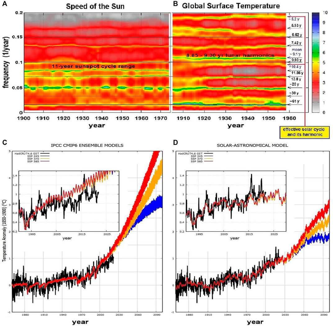
FIGURE 6. (A) Time-frequency analysis (L = 110 years) of the speed of the Sun relative to the barycenter of the solar system. (B) Time frequency analysis (L = 110 years) of the detrended HadCRUT3 temperature record. (cf. Scafetta, 2014b). (C) Ensemble CMIP6 GCM mean simulations for different emission scenarios versus the HadCRUT global surface temperatures. (D) The same record compared with the solar-astronomical harmonic climate model Scafetta (2013) updated in Scafetta (2021).

Evidences for a astronomical origin of the Sub-Milankovitch climate oscillations have been discussed in several studies (e.g.: Scafetta, 2010; 2014b, 2016, 2018, 2021). Let us now summarizes the main findings relative to the global surface temperature record from 1850 to 2010.

Figures 6A,B compare the time-frequency analyses between the speed of the Sun relative to the center of mass of the solar system (Figure 1) and the HadCRUT3 global surface records (Scafetta, 2014b). It can be seen that the global surface temperature oscillations mimic several astronomical cycles at the decadal and multidecadal scales, as first noted in Scafetta (2010) and later confirmed by advanced spectral coherence analyses (Scafetta, 2016, 2018).

The main periods found in the speed of the Sun (Figure 6A) are at about 5.93, 6.62, 7.42, 9.93, 11.86, 13.8, 20 and 60 years. Most of them are related to the orbits of Jupiter and Saturn. The main periods found in the temperature record (Figure 6B) are at about 5.93, 6.62, 7.42, 9.1, 10.4, 13.8, 20 and 60 years. Most of these periods appear to coincide with orbital invariant inequalities (Table 6) but the 9.1 and 10.4-year cycles.

Among the climate cycles, it is also found an important period of about 9.1 years, which is missing among the main planetary frequencies shown in Figure 6A. Scafetta (2010) argued that this oscillation is likely linked to a combination of the 8.85-year lunar apsidal line rotation period, the first harmonic of the 9-year Saros eclipse cycle and the 9.3-year first harmonic of the soli-lunar nodal cycle (Cionco et al., 2021; Scafetta, 2012d, supplement). These three lunar cycles induce oceanic tides with an average period of about 9.1 years (Wood, 1986; Keeling and Whorf, 2000) that could affect the climate system by modulating the atmospheric and oceanic circulation.

The 10.4-year temperature cycle is variable and appears to be the signature of the 11-year solar cycle that varies between the Jupiter-Saturn spring tidal cycle (9.93 years) and the orbital period of Jupiter (11.86 years). Note that in Figure 6B, the frequency of this temperature signal increased in time from 1900 to 2000. This agrees with the solar cycle being slightly longer (and smaller) at the beginning of the 20th century and shorter (and larger) at its end (see Figure 2). We also notice that the 10.46-year period corresponds to the orbital invariant inequality (3, −5, 3, −1) among Venus, Earth, Jupiter and Saturn.

The above findings were crucial for the construction of a semi-empirical climate model based on the several astronomically identified cycles (Scafetta, 2010, 2013). The model included the 9.1-year solar-lunar cycle, the astronomical-solar cycles at 10.5, 20, 60 and, in addition, two longer cycles with periods of 115 years (using Eq. 25) and a millennial cycle here characterized by an asymmetric 981-year cycle with a minimum around 1700 (the Maunder Minimum) and two maxima in 1080 and 2060 (using Eq. 28). The model was completed by adding the volcano and the anthropogenic components deduced from the ensemble average prediction of the CMIP5 global circulation models assuming an equilibrium climate sensitivity (ECS) of about 1.5°C that is half of that of the model average, which is about 3°C. This operation was necessary because the identified natural oscillations already account for at least 50% of the warming observed from 1970 to 2000. Recently, Scafetta (2021) upgraded the model by adding some higher frequency cycles.

Figure 6C shows the HadCRUT4.6 global surface temperature record (Morice et al., 2012) against the ensemble average simulations produced by the CMIP6 global circulation models (GCMs) using historical forcings (1850–2014) extended with three different shared socioeconomic pathway (SSP) scenarios (2015–2100) (Eyring et al., 2016). Figure 6D shows the same temperature record against the proposed semi-empirical astronomical harmonic model under the same forcing conditions. The comparison between panels C and D shows that the semi-empirical harmonic model performs significantly better than the classical GCMs in hindcasting the 1850–2020 temperature record. It also predicts moderate warming for the future decades, as explained in detail by Scafetta (2013, 2021).

10 Possible Physical Mechanisms

Many authors suggest that solar cycles revealed in sunspot and cosmogenic records could derive from a deterministic non-linear chaotic dynamo (Weiss and Tobias, 2016; Charbonneau, 2020, 2022). However, the assumption that solar activity is only regulated by dynamical and stochastic processes inside the Sun has never been validated mainly because these models have a poor hindcasting capability.

We have seen how the several main planetary harmonics and orbital invariant inequalities tend to cluster towards specific frequencies that characterize the observed solar activity cycles. This suggests that the strong synchronization among the planetary orbits could be further extended to the physical processes that are responsible for the observed solar variability.

The physical mechanisms that could explain how the planets may directly or indirectly influence the Sun are currently unclear. It can be conjectured that the solar dynamo might have been synchronized to some planetary periods under the action of harmonic forcings acting on it for several hundred million or even billion years. In fact, as pointed out by Huygens in the 17th century, synchronization can occur even if the harmonic forcing is very weak but lasts long enough (Pikovsky et al., 2001).

There may be two basic types of mechanisms referred to how and where in the Sun the planetary forcing is acting. In particular, we distinguish between the mechanisms that interact with the outer regions of the Sun and those that act in its interior.

1. Planetary tides can perturb the surface magnetic activity of the Sun, the solar corona, and thus the solar wind. The solar wind, driven by the rotating twisted magnetic field lines (Parker, 1958; Tattersall, 2013), can reconnect with the magnetic fields of the planets when they get closer during conjunctions. This would modulate the solar magnetic wind density distribution and the screening efficiency of the whole heliosphere on the incoming cosmic rays. The effect would be a modulation of the cosmogenic records which then also act on the cloud cover. It is also possible that the planets can focus and modulate by gravitational lensing the flux of interstellar and interplanetary matter–perhaps even of dark matter–towards the Sun and the Earth stimulating solar activity (Bertolucci et al., 2017; Scafetta, 2020; Zioutas et al., 2022) and, again, contributing to clouds formation on Earth which alters the climate.

2. Gravitational planetary tides and torques could reach the interior of the Sun and synchronize the solar dynamo by forcing its tachocline (Abreu et al., 2012; Stefani et al., 2016, 2019, 2021) or even modulate the nuclear activity in the core (Wolff and Patrone, 2010; Scafetta, 2012b).

Scafetta and Willson (2013b) argued that these two basic mechanisms could well complement each other. In principle, it might also be possible that the physical solar dynamo is characterized by a number of natural frequencies that could resonate with the external periodic forcings yielding some type of synchronization. Let us briefly analyze several cases.

10.1 Mechanisms Associated With Planetary Alignments

The frequencies associated with planetary alignments and, in particular, those of the Jovian planets, were found to reproduce the main observed cycles in solar and climatic data. Scafetta (2020) showed examples of gravitational field configurations produced by a toy-model made of four equal masses orbiting around a 10 times more massive central body.

The Sun could feel planetary conjunctions because at least twenty-five out of thirty-eight largest solar flares were observed to start when one or more planets among Mercury, Venus, Earth, and Jupiter were either nearly above the position of the flare (within 10° longitude) or on the opposite side of the Sun (Hung, 2007). For example, Mörner et al. (2015) showed that, on 7 January 2014, a giant solar flare of class X1.2 was emitted from the giant sunspot active region AR 1944 (NASA, 2014), and that the flare pointed directly toward the Earth when Venus, Earth and Jupiter were exactly aligned in a triple conjunction and the planetary tidal index calculated by Scafetta (2012b) peaked at the same time.

Hung (2007) estimated that the probability for this to happen at random was 0.039%, and concluded that “the force or momentum balance (between the solar atmospheric pressure, the gravity field, and magnetic field) on plasma in the looping magnetic field lines in solar corona could be disturbed by tides, resulting in magnetic field reconnection, solar flares, and solar storms.” Comparable results and confirmations that solar flares could be linked to planetary alignments were recently discussed in Bertolucci et al. (2017) and Petrakou (2021).

10.2 Mechanisms Associated With the Solar Wobbling

The movement of the planets and, in particular, of the Jovian ones, are reflected in the solar wobbling. Charvátová (2000) and Charvátová and Hejda (2014) showed that the solar wobbling around the center of mass of the solar system forms two kinds of complex trajectories: an ordered one, where the orbits appear more symmetric and circular, and a disordered type, where the orbits appear more eccentric and randomly distributed. These authors found that the alternation between these two states presents periodicities related, for example, to the Jose (∼178 years) and Bray–Hallstatt (∼2300 years) cycles.

Figure 7A compares the Bray–Hallstatt cycle found in the Δ¹⁴C (‰) record (black) throughout the Holocene (Reimer et al., 2004, IntCal04.14c) with two orbital records representing the periods of the pericycle and apocycle orbital arcs of the solar trajectories as extensively discussed by Scafetta et al. (2016). Figure 7B shows the solar wobbling for about 6000 years where the alternation of ordered and disordered orbital patterns typically occurs according to the Bray–Hallstatt cycle of 2318 years (Scafetta et al., 2016).

FIGURE 7

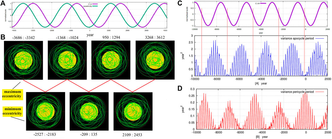
FIGURE 7. (A) The Hallstatt oscillation (2318 years) found in Δ¹⁴C (‰) record and in the eccentricity function of the barycenter of the planets relative to the Sun. (B) Ordered and disordered orbits of the barycenter of the planets relative to the Sun. (C,D) The Hallstatt oscillation found in Δ¹⁴C (‰) record and in the apocycles and pericycles of the orbits of the center of mass of the planets relative to the Sun. (cf. Scafetta et al., 2016).

In particular, the astronomical records show that the Jose cycle is modulated by the Bray–Hallstatt cycle. Figures 7C,D show examples of how planetary configurations can reproduce the Bray–Hallstatt cycle: see details in Scafetta et al. (2016). The fast oscillations correspond to the orbital invariant inequalities with periods of 159, 171.4 and 185 years while the long beat oscillation corresponds to the orbital invariant inequality with a period of 2318 years, which perfectly fits the Bray–Hallstatt cycle as estimated in McCracken et al. (2013) (see Table 6). It is possible that the pulsing dynamics of the heliosphere can periodically modulate the solar wind termination shock layer and, therefore, the incoming interstellar dust and cosmic ray fluxes.

10.3 Mechanisms Associated With Planetary Tides and Tidal Torques

Discussing the tidal interactions between early-type binaries, Goldreich and Nicholson (1989) demonstrated that the tidal action and torques can produce important effects in the thin overshooting region between the radiative and the convective zone, which is very close to the tachocline. This would translate both in tidal torques and in the onset of g-waves moving throughout the radiative region. A similar mechanism should also take place in late-type stars like the Sun (Goodman and Dickson, 1998).

Abreu et al. (2012) found an excellent agreement between the long-term solar cycles and the periodicities in the planetary tidal torques. These authors assumed that the solar interior is characterized by a non-spherical tachocline. Under such a condition, the planetary gravitational forces exert a torque on the tachocline itself that would then vary with the distribution of the planets around the Sun. These authors showed that the torque function is characterized by some specific planetary frequencies that match those observed in cosmogenic radionuclide proxies of solar activity. The authors highlighted spectral coherence at the following periods: 88, 104, 150, 208 and 506 years. The first four periods were discussed above using alternative planetary functions; the last period could be a harmonic of the millennial solar cycle also discussed above and found in the same solar record (Scafetta, 2012a; 2014b).

Abreu et al. (2012) observed that the tachocline approximately coincides with the layer at the bottom of the convection zone where the storage and amplification of the magnetic flux tubes occur. These are the flux tubes that eventually erupt at the solar photosphere to form active regions. The tachocline layer is in a critical state because it is very sensitive to small perturbations being between the radiative zone characterized by stable stratification (δ < 0) and the convective zone characterized by unstable stratification (δ > 0). The proposed hypothesis is that the planetary tides could influence the magnetic storage capacity of the tachocline region by modifying its entropy stratification and the superadiabaticity parameter δ, thereby altering the maximum field strength of the magnetic flux tubes that regulate the solar dynamo.

However, Abreu et al. (2012) also acknowledged that their hypothesis could not explain how the tiny tidal modification of the entropy stratification could produce an observable effect although they conjectured the presence of a resonance mediated by gravity waves.

The planetary tidal influence on the solar dynamo has been rather controversial because the tidal accelerations at the tachocline layer are about 1000 times smaller than the accelerations of the convective cells (de Jager and Versteegh, 2005). Scafetta (2012b) calculated that the gravitational tidal amplitudes produced by all the planets on the solar chromosphere are of the order of 1 mm or smaller (see Table 7). More recently, Charbonneau (2022) critiqued Stefani et al. (2019, 2021) by observing that also the planetary tidal forcings of Jupiter and Venus could only exert a “homeopathic” influence on the solar tachocline concluding that they should be unable to synchronize the dynamo. Charbonneau (2022) also observed that even angular momentum transport by convective overshoot into the tachocline would be inefficient and concluded that synchronization could only be readily achieved in presence of high forcing amplitudes, stressing the critical need for a powerful amplification mechanism.

TABLE 7

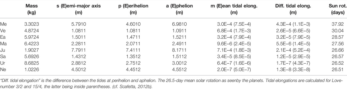
TABLE 7. Mean tidal elongations at the solar surface produced by all planets.

While it is certainly true that the precise underlying mechanism is not completely understood, the rough energetic estimate that 1 mm tidal height corresponds to 1 m/s velocity at the tachocline level might still entail sufficient capacity for synchronization by changing the (sensitive) field storage capacity (Abreu et al., 2012) or by synchronizing that part of α that is connected with the Tayler instability or by the onset of magneto-Rossby waves at the tachocline (Dikpati et al., 2017; Zaqarashvili, 2018). In all cases, it could be possible that only a few high-frequency planetary forcing (e.g. the 11.07-year Venus-Earth-Jupiter tidal model) are able to efficiently synchronize the solar dynamo (Stefani et al., 2016; Stefani et al., 2018; Stefani et al., 2019). At the same time, additional and longer solar cycles could emerge when some feature of the dynamo is also modulated by the angular momentum exchange associated with the solar wobbling (Stefani et al., 2021). Finally, Albert et al. (2021) proposed that stochastic resonance could explain the multi-secular variability of the Schwabe cycle by letting the dynamo switch between two distinct operating modes as the solution moves back and forth from the attraction basin of one to the other.

Alternatively, the problem of the tidal “homeopathic” influence on the tachocline could be solved by observing that tides could play some more observable role in the large solar corona where the solar wind originates, or in the wind itself at larger distances from the Sun where the tides are stronger, or even in the solar core where they could actually trigger a powerful response from nuclear fusion processes. Let us discuss the latter hypothesis.

10.4 A Possible Solar Amplification of the Planetary Tidal Forcing

A possible amplification mechanism of the effects of the tidal forcing was introduced by Wolff and Patrone (2010) and Scafetta (2012b).

Wolff and Patrone (2010) proposed that tidal forcing could act inside the solar core inducing waves in the plasma by mixing the material and carrying fresh fuel to the deeper and hotter regions. This mechanism would make solar-type stars with a planetary system slightly brighter because their fuel would burn more quickly.

Scafetta (2012b) further developed this approach and introduced a physical mechanism inspired by the mass-luminosity relation of main-sequence stars. The basic idea is that the luminosity of the core of the Sun can be written as

$L\left(t\right)\approx L_{\odot }+A\cdot {\dot{\mathrm{\Omega }}}_{\mathit{tidal}}\left(t\right),(47)$

where L_⊙ is the baseline luminosity of the star without planets and $\mathrm{\Delta }{L}_{\mathit{tidal}}(t)=A\cdot {\dot{\mathrm{\Omega }}}_{\mathit{tidal}}(t)$ is the small luminosity increase induced by planetary tides inside the Sun. ${\dot{\mathrm{\Omega }}}_{\mathit{tidal}}(t)$ is the rate of the gravitational tidal energy which is continuously dissipated in the core and A is the amplification factor related to the triggered luminosity production via H-burning.

To calculate the magnitude of the amplification factor A we start by considering the Hertzsprung-Russell mass-luminosity relation, which establishes that, if the mass of a star increases, its luminosity L, increases as well. In the case of a G-type main-sequence star, with luminosity L and mass M = M_⊙ + ΔM, the mass-luminosity relation approximately gives

$\frac{L}{L_{\odot }}\approx {\left(\frac{M}{M_{\odot }}\right)}^4\approx 1+\frac{4\mathrm{\Delta }M}{M_{\odot }},(48)$

where L_⊙ is the solar luminosity and M_⊙ is the mass of the Sun (Duric, 2004). By relating the luminosity of a star to its mass, the Hertzsprung-Russell relation suggests a link between the luminosity and the gravitational power continuously dissipated inside the star.

The total solar luminosity is

$L_{\odot }=4\pi {\left(1AU\right)}^2\times TSI=3.827\cdot 10^{26}W,(49)$

where 1 AU = 1.496 ⋅ 10¹¹ m is the average Sun-Earth distance, and TSI is the total solar irradiance 1360.94 W/m² at 1 AU. Every second, the core of the Sun transforms into luminosity a certain amount of mass according to the Einstein equation E = mc². If dL(r) is the luminosity produced inside the shell between r and r + dr (Bahcall et al., 2001, 2005), the mass transformed into light every second in the shell is

$\frac{d\dot{m}\left(r\right)}{dr}=\frac{1}{c^2}\frac{dL\left(r\right)}{dr},(50)$

where c = 2.998 ⋅ 10⁸ m/s is the speed of the light and r is the distance from the center of the Sun.

The transformed material can be associated with a correspondent loss of gravitational energy of the star per time unit ${\dot{U}}_{\odot }$, which can be calculated using Eq. 50 as

${\dot{U}}_{\odot }=\frac{1}{2}G{\int }_0^{R_S}{m}_{\odot }\left(r\right)\frac{d\dot{m}\left(r\right)}{dr}\frac{1}{r}dr=\frac{1}{2}\frac{G}{c^2}{\int }_0^{R_S}{m}_{\odot }\left(r\right)\frac{dL\left(r\right)}{dr}\frac{1}{r}dr=3.6\cdot 10^{20}W,(51)$

where the initial factor 1/2 is due to the virial theorem, m_⊙(r) is the solar mass within the radius r ≤ R_S and L(r) is the luminosity profile function derived by the standard solar model (Bahcall et al., 2001, 2005).

The gravitational forces will do the work necessary to compensate for such a loss of energy to restore the conditions for the H-burning. In fact, the solar luminosity would decrease if the Sun’s gravity did not fill the vacuum created by the H-burning, which reduces the number of particles by four (4H → 1He). At the same time, the nucleus of He slowly sinks releasing additional potential energy. All this corresponds to a gravitational work in the core per time unit, ${\dot{\mathrm{\Omega }}}_{\odot }$ that is associated with light production.

The basic analogy made by Scafetta (2012b) is that ${\dot{\mathrm{\Omega }}}_{\odot }$ should be of the same order of magnitude as the rate of the gravitational energy loss due to H-fusion $({\dot{\mathrm{\Omega }}}_{\odot }\approx {\dot{U}}_{\odot })$. Moreover, the energy produced by the dissipation of the tidal forces in the core should be indistinguishable from the energy produced by the other gravitational forces in the Sun. Thus, it is as if tides added some gravitational power that becomes ${\dot{\mathrm{\Omega }}}_{\odot }+{\dot{\mathrm{\Omega }}}_{\mathit{tidal}}$.

For small perturbations, since light production is directly related both to the solar mass and to the gravitational power dissipated inside the core, Scafetta (2012b) assumed the equivalence

$\frac{\mathrm{\Delta }M}{M_{\odot }}\equiv \frac{{\dot{\mathrm{\Omega }}}_{\mathit{tidal}}}{{\dot{\mathrm{\Omega }}}_{\odot }},(52)$

where ${\dot{\mathrm{\Omega }}}_{\mathit{tidal}}$ is the tidal perturbing power dissipated inside the Sun and ${\dot{\mathrm{\Omega }}}_{\odot }\equiv {\dot{U}}_{\odot }$ is the rate of the gravitational energy lost by the Sun through H-burning. Thus, from Eqs 47, 48 we get

$L\left(t\right)\approx L_{\odot }+\frac{4L_{\odot }}{{\dot{\mathrm{\Omega }}}_{\odot }}{\dot{\mathrm{\Omega }}}_{\mathit{tidal}}\left(t\right)=L_{\odot }+A\cdot {\dot{\mathrm{\Omega }}}_{\mathit{tidal}}\left(t\right),(53)$

where the amplification factor is calculated as

$A=4\frac{L_{\odot }}{{\dot{\mathrm{\Omega }}}_{\odot }}\approx 4\frac{L_{\odot }}{{\dot{U}}_{\odot }}\approx 4.25\cdot 10^6.(54)$

Equation 54 means that any little amount of gravitational power dissipated in the core (like that induced by planetary tidal forcing) could be amplified by a factor of the order of one million by nuclear fusion. This could be equivalent to having gravitational tidal amplitudes amplified from 1 mm to 1 km at the tachocline. This amplification could solve the problem of the “homeopathic” gravitational tidal energy contribution highlighted by Charbonneau (2022).

By using such a large amplification factor and the estimated gravitational power ${\dot{\mathrm{\Omega }}}_{\mathit{tidal}}$ dissipated inside the solar core, Scafetta (2012b) calculated the tidally-induced TSI produced by each of the planets (Figures 8A,B), as well as that of all the planets together (Figure 8C). The sequence of the relative tidal relevance of the planets is Jupiter, Venus, Earth, Mercury, Saturn, Mars, Uranus and Neptune. The mean enhancement of their overall tidally-induced TSI is of the order of 0.3–0.8 W/m², depending on the specific Love number of the tides (see Figure 8C). However, on shorter time scales the tides could produce TSI fluctuations up to 0.6–1.6 W/m² in absence of dampening mechanisms. In particular, on a decadal time scale, the TSI fluctuations due to Jupiter and Saturn could reach amplitudes of 0.08–0.20 W/m² (see the black curve in Figure 8C).

FIGURE 8

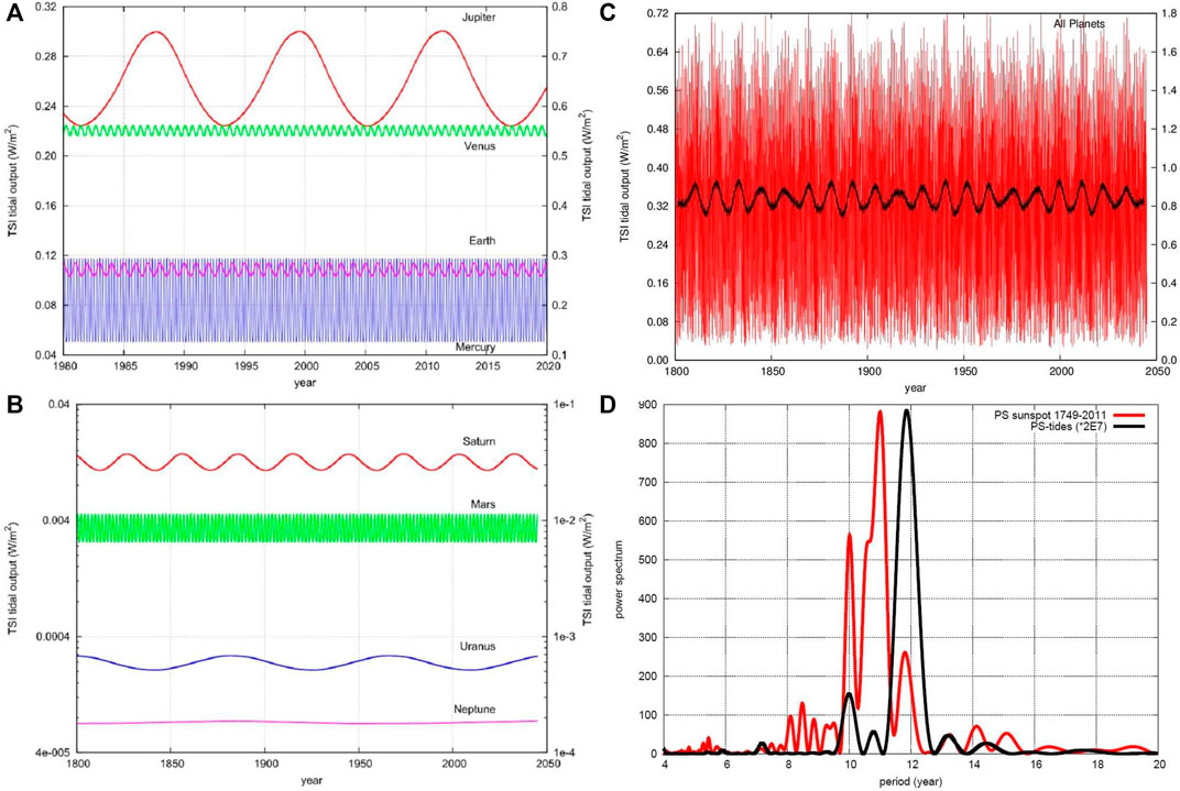
FIGURE 8. (A,B) Theoretical TSI enhancement induced by the tides of each planet on the Sun obtained using Scafetta (2012b) amplification hypothesis; the Love numbers are 3/2 (left axis) and 15/4 (right axis). (C) The same as produced by the tides of all the planets. (D) Lomb-periodogram spectral analysis of the sunspot number record (red) and of the tidal function (black) produced by all the planets.

If the luminosity flux reaching the tachocline from the radiative zone is modulated by the contribution of tidally-induced luminosity oscillations with a TSI amplitude of the order of 0.01-0.10 W/m², the perturbation could be sufficiently energetic to tune the solar dynamo with the planetary frequencies. The dynamo would then further amplify the luminosity signal received at the tachocline up to $\sim 1W/m^2$ amplitudes as observed in TSI cycles (Willson and Mordvinov, 2003).

Figure 8D compares the periodograms of the sunspot number record and of the planetary luminosity signal shown in Figure 8C. The two side frequency peaks at about 10 years (J/S-spring tide) and 11.86 years (J-tide) perfectly coincide in the two spectral analyses. The central frequency peak at about 10.87 years shown only by sunspot numbers could be directly generated by the solar dynamo excited by the two tidal frequencies (Scafetta, 2012a) or other mechanisms connected with the dynamo as discussed above.

An obvious objection to the above approach is that the Kelvin-Helmholtz time-scale (Mitalas and Sills, 1992; Stix, 2003) predicts that the light journey from the core to the convective zone requires 10⁴–10⁸ years. Therefore, the luminosity fluctuations produced inside the core could be hardly detectable because they would be smeared out before reaching the convective zone. At most, there could exist only a slightly enhanced solar luminosity related to the overall tidally-induced TSI mean enhancement of the order of 0.3–0.8 W/m² as shown in Figure 8C.

However, several different mechanisms may be at work. In fact, the harmonic tidal forcing acts simultaneously throughout the core and in the radiative zone, and simultaneously produces everywhere a synchronized energy oscillation that can be amplified in the core as discussed above. This would can give rise to modulated seismic waves (g and p-mode oscillations) that can propagate from the core up to the tachocline region in a few hours because the sound speed inside the Sun is a few hundred kilometers per second (Hartlep and Mansour, 2005; Barker and Ogilvie, 2010; Ahuir et al., 2021). These waves might also couple with the g-waves produced in the tachocline (Goodman and Dickson, 1998) producing a perturbation in the tachocline region sufficiently strong to synchronize the solar dynamo with the planetary tidal frequencies.

11 Conclusion

Many empirical evidences suggest that planetary systems can self-organize in synchronized structures although some of the physical mechanisms involved are still debated.

We have shown that the high synchronization of our own planetary system is nicely revealed by the fact that the ratios of the orbital radii of adjacent planets, when raised to the 2/3rd power, express the simple ratios found in harmonic musical consonances while those of the mirrored ones follow the simple, elegant, and highly precise scaling-mirror symmetry Eq. 1 (Bank and Scafetta, 2022).

The solar system is made of synchronized coupled oscillators because it is characterized by a set of frequencies that are linked to each other by the harmonic Eq. 3, which are easily detected in the solar wobbling. Thus, it is then reasonable to hypothesize that the solar activity could be also tuned to planetary frequencies.

We corroborated this hypothesis by reviewing the many planetary harmonics and orbital invariant inequalities that characterize the planetary motions and observing that often their frequencies correspond to those of solar variability.

It may be objected that, since the identified planetary frequencies are so numerous, it could be easy to occasionally find that some of them roughly correspond to those of the solar cycles. However, the fact is that the planetary frequencies of the solar system, from the monthly to the millennial time scales, are not randomly distributed but tend to cluster around some specific values that quite well match those of the main solar activity cycles.

Thus, it is rather unlikely that the results shown in Figures 2–6 are just occasional. In some cases, our proposed planetary models have even been able to predict the time-phase of the solar oscillations like that of the Schwabe 11-year sunspot cycle throughout the last three centuries, as well as those of the secular and millennial modulations throughout the Holocene. The two main planetary models that could explain the Schwabe 11-year cycle and its secular and millennial variation involve the planets Venus, Earth, Jupiter and Saturn, as it was initially suggested by Wolf (1859). We further suggest that the Venus-Earth-Jupiter model and the Jupiter-Saturn model could be working complementary to each other.

The alternative hypothesis that the solar activity is regulated by an unforced internal dynamics alone (i.e. by an externally unperturbed solar dynamo) has never been able to reproduce the variety of the observed oscillations. In fact, standard MHD dynamo models are not self-consistent and do not even directly explain the well-known 11-year solar cycle nor they are able to predict its timing without assuming a number of calibrated parameters (Tobias, 2002; Jiang et al., 2007).

There have been several objections to a planetary theory of solar variability. For example, Smythe and Eddy (1977) claimed that planetary cycles and conjunctions could not predict the timing of grand solar minima like the Maunder Minimum of the 17th century. However, Scafetta (2012a) developed a solar-planetary model able to predict all the grand solar maxima and minima of the last millennium (Figure 4).

Other authors reasonably claimed that planetary gravitational tides are too weak to modulate solar activity (Charbonneau, 2002; de Jager and Versteegh, 2005; Charbonneau, 2022); yet, several empirical evidences support the importance of their role (Wolff and Patrone, 2010; Abreu et al., 2012; Scafetta, 2012b; Stefani et al., 2016, 2019). Stefani et al. (2016, 2021) proposed that the Sun could be at least synchronized by the tides of Venus, Earth and Jupiter, producing an 11.07-year cycle that reasonably matches the Schwabe cycle. Longer cycles could be produced by a dynamo excited by angular momentum transfer from Jupiter and Saturn. Instead, Scafetta (2012b) proposed that, in the solar core, the effects of the weak tidal forces could be amplified one million times or more due to an induced increase in the H-burning, thus providing a sufficiently strong forcing to synchronize and modulate the solar dynamo with planetary harmonics at multiple time scales.

Objections to the latter hypothesis, based on the slow light propagation inside the radiative zone according to the Kelvin–Helmholtz timescale (Mitalas and Sills, 1992; Stix, 2003), could be probably solved. In fact, tidal forces are believed to favor the onset of g-waves moving back and forth throughout the radiative region of the Sun (Barker and Ogilvie, 2010; Ahuir et al., 2021). Thus, g-waves themselves could be amplified and modulated in the core by the tidally induced H-burning enhancement (Scafetta, 2012b). Then, both tidal torques and g-waves could cyclically affect the tachocline region at the bottom of the convective zone and synchronize the solar dynamo.

Alternatively, planetary alignments can also modify the large-scale electromagnetic and gravitational structure of the planetary system altering the space weather in the solar system. For example, in coincidence of planetary alignments, an increase of solar flares has been observed (Hung, 2007; Bertolucci et al., 2017; Petrakou, 2021). The solar wobbling, which reflects the motion of the barycenter of the planets, changing from more regular to more chaotic trajectories, correlates well with some long climate cycles like the Bray-Hallstatt cycle (2100–2500 years) (Charvátová, 2000; Charvátová and Hejda, 2014; Scafetta et al., 2016). Finally, Scafetta et al. (2020) showed that the infalling meteorite flux on the Earth presents a 60-year oscillation coherent with the variation of the eccentricity of Jupiter’s orbit induced by Saturn. The falling flux of meteorites and interplanetary dust would then contribute to modulate cloud formation.

In conclusion, many empirical evidences suggest that planetary oscillations should be able to modulate the solar activity and even the Earth’s climate, although several open physical issues remain open. These results stress the importance of identifying the relevant planetary harmonics, the solar activity cycles and the climate oscillations as phenomena that, in many cases, are interconnected. This approach could be useful to predict both solar and climate variability using harmonic constituent models as it is currently done for oceanic tides. We think that the theory of a planetary modulation of solar activity should be further developed because no clear alternative theory exists to date capable to explain the observed planetary-solar interconnected periodicities.

Author Contributions

NS wrote a first draft of the paper. NS and AB have discussed in more details all the topics and together prepared the final manuscript.

Conflict of Interest

The authors declare that the research was conducted in the absence of any commercial or financial relationships that could be construed as a potential conflict of interest.

Publisher’s Note

All claims expressed in this article are solely those of the authors and do not necessarily represent those of their affiliated organizations, or those of the publisher, the editors and the reviewers. Any product that may be evaluated in this article, or claim that may be made by its manufacturer, is not guaranteed or endorsed by the publisher.

References

Abreu, J. A., Beer, J., Ferriz-Mas, A., McCracken, K. G., and Steinhilber, F. (2012). Is There a Planetary Influence on Solar Activity? Astronomy Astrophysics 548, A88. doi:10.1051/0004-6361/201219997

CrossRef Full Text | Google Scholar

Agnihotri, R., and Dutta, K. (2003). Centennial Scale Variations in Monsoonal Rainfall (Indian, East Equatorial and Chinese Monsoons): Manifestations of Solar Variability. Curr. Sci. 85, 459–463.

Google Scholar

Agol, E., Dorn, C., Grimm, S. L., Turbet, M., Ducrot, E., Delrez, L., et al. (2021). Refining the Transit-Timing and Photometric Analysis of TRAPPIST-1: Masses, Radii, Densities, Dynamics, and Ephemerides. Planet. Sci. J. 2, 1. doi:10.3847/psj/abd022

CrossRef Full Text | Google Scholar

Ahuir, J., Mathis, S., and Amard, L. (2021). Dynamical Tide in Stellar Radiative Zones. Astronomy Astrophysics 651, A3.

Google Scholar

Albert, C., Ferriz-Mas, A., Gaia, F., and Ulzega, S. (2021). Can Stochastic Resonance Explain Recurrence of Grand Minima? ApJL 916, L9. doi:10.3847/2041-8213/ac0fd6

CrossRef Full Text | Google Scholar

Aschwanden, M. J. (2018). Self-organizing Systems in Planetary Physics: Harmonic Resonances of Planet and Moon Orbits. New Astron. 58, 107–123. doi:10.1016/j.newast.2017.08.002

CrossRef Full Text | Google Scholar

Bahcall, J. N., Pinsonneault, M. H., and Basu, S. (2001). Solar Models: Current Epoch and Time Dependences, Neutrinos, and Helioseismological Properties. Astrophysical J. 555, 990–1012. doi:10.1086/321493

CrossRef Full Text | Google Scholar

Bahcall, J. N., Serenelli, A. M., and Basu, S. (2005). New Solar Opacities, Abundances, Helioseismology, and Neutrino Fluxes. Astrophysical J. 621, L85–L88. doi:10.1086/428929

CrossRef Full Text | Google Scholar

Bank, M. J., and Scafetta, N. (2022). Scaling, Mirror Symmetries and Musical Consonances Among the Distances of the Planets of the Solar System. Front. Astron. Space Sci. 8, 758184. doi:10.3389/fspas.2021.758184

CrossRef Full Text | Google Scholar

Bard, E., Raisbeck, G., Yiou, F., and Jouzel, J. (2000). Solar Irradiance during the Last 1200 Years Based on Cosmogenic Nuclides. Tellus B 52, 985–992. doi:10.1034/j.1600-0889.2000.d01-7.x

CrossRef Full Text | Google Scholar

Barker, A. J., and Ogilvie, G. I. (2010). On Internal Wave Breaking and Tidal Dissipation Near the Centre of a Solar-type Star. Mon. Notices R. Astronomical Soc. 404, 1849–1868. doi:10.1111/j.1365-2966.2010.16400.x

CrossRef Full Text | Google Scholar

Bartels, J. (1934). Twenty-seven Day Recurrences in Terrestrial-Magnetic and Solar Activity, 1923-1933. J. Geophys. Res. 39, 201–202a. doi:10.1029/TE039i003p00201

CrossRef Full Text | Google Scholar

Battistini, A. (2011). Il ciclo undecennale del sole secondo Bendandi (The 11-year solar cycle according to Bendandi). New Ice Age. Available at: http://daltonsminima.altervista.org/?p=8669.

Google Scholar

Beck, J. G. (2000). A Comparison of Differential Rotation Measurements. Sol. Phys. 191, 47–70. doi:10.1023/a:1005226402796

CrossRef Full Text | Google Scholar

Beer, J., Tobias, S. M., and Weiss, N. O. (2018). On Long-Term Modulation of the Sun's Magnetic Cycle. Mon. Not. R. Astron. Soc. 473, 1596–1602. doi:10.1093/mnras/stx2337

CrossRef Full Text | Google Scholar

Bendandi, R. (1931). Un Principio Fondamentale dell’Universo (A Fundamental Principle of the Universe). Faenza: Osservatorio Bendandi.

Google Scholar

Bertolucci, S., Zioutas, K., Hofmann, S., and Maroudas, M. (2017). The Sun and its Planets as Detectors for Invisible Matter. Phys. Dark Universe 17, 13–21. doi:10.1016/j.dark.2017.06.001

CrossRef Full Text | Google Scholar

Bigg, E. K. (1967). Influence of the Planet Mercury on Sunspots. Astronomical J. 72, 463–466. doi:10.1086/110250

CrossRef Full Text | Google Scholar

Bollinger, C. J. (1952). A 44.77 Year Jupiter-Earth-Venus Configuration Sun-Tide Period in Solar-Climate Cycles. Acad. Sci. 1952 – Proc. Okla. 1952, 307–311. Available at: http://digital.library.okstate.edu/oas/oas_pdf/v33/v307_311.pdf.

Google Scholar

Brown, E. W. (1900). A Possible Explanation of the Sun-Spot Period. Mon. Notices R. Astronomical Soc. 60, 599–606. doi:10.1093/mnras/60.10.599

CrossRef Full Text | Google Scholar

Bucha, V., Jakubcová, I., Pick, M., and Šimon, Z. (1985). Resonance Frequencies in the Sun's Motion. Stud. Geophys Geod. 29, 107–111. doi:10.1007/bf01585713

CrossRef Full Text | Google Scholar

Cauquoin, A., Raisbeck, G. M., Jouzel, J., Bard, E., and ASTER Team, (2014). No Evidence for Planetary Influence on Solar Activity 330 000 Years Ago. Astronomy Astrophysics 561, A132. doi:10.1051/0004-6361/201322879

CrossRef Full Text | Google Scholar

Chang, S., and Yu, Z. (1981). Historical Records of Meteorite Falls in China and Their Time Series Analysis. Natl. Inst. Polar Res. Memoirs, Special Issue 20, 276–284.

Google Scholar

Charbonneau, P. (2020). Dynamo Models of the Solar Cycle. Living Rev. Sol. Phys. 17, 4. doi:10.1007/s41116-020-00025-6

CrossRef Full Text | Google Scholar

Charbonneau, P. (2022). External Forcing of the Solar Dynamo. Front. Astron. Space Sci. 9, 853676. doi:10.3389/fspas.2022.853676

CrossRef Full Text | Google Scholar

Charbonneau, P. (2002). The Rise and Fall of the First Solar Cycle Model. J. Hist. Astronomy 33 (4), 351–372. doi:10.1177/002182860203300402

CrossRef Full Text | Google Scholar

Charvátová, I. (2000). Can Origin of the 2400-year Cycle of Solar Activity Be Caused by Solar Inertial Motion? Ann. Geophys. 18, 399–405. doi:10.1007/s00585-000-0399-x

CrossRef Full Text | Google Scholar

Charvátová, I., and Hejda, P. (2014). Responses of the Basic Cycles of 178.7 and 2402 Yr in Solar-Terrestrial Phenomena during the Holocene. Pattern Recogn. Phys. 2, 21–26. doi:10.5194/PRP-2-21-2014

CrossRef Full Text | Google Scholar

Cionco, R. G., Kudryavtsev, S. M., and Soon, W. W.-H. (2021). Possible Origin of Some Periodicities Detected in Solar-Terrestrial Studies: Earth’s Orbital Movements. Earth Space Sci. 8, e2021EA001805. doi:10.1029/2021ea001805

CrossRef Full Text | Google Scholar

Cionco, R. G., and Pavlov, D. A. (2018). Solar Barycentric Dynamics from a New Solar-Planetary Ephemeris. Astronomy Astrophysics 615, A153. doi:10.1051/0004-6361/201732349

CrossRef Full Text | Google Scholar

Cole, L. C., and Bushby, P. J. (2014). Modulated Cycles in an Illustrative Solar Dynamo Model with Competingα-Effects. Astronomy Astrophysics 563, A116. doi:10.1051/0004-6361/201323285

CrossRef Full Text | Google Scholar

de Jager, C., and Versteegh, G. J. M. (2005). Do Planetary Motions Drive Solar Variability? Sol. Phys. 229, 175–179. doi:10.1007/s11207-005-4086-7

CrossRef Full Text | Google Scholar

de Vries, H. (1958). Variations in Concentration of Radiocarbon with Time and Location on Earth. Proc. K. Ned. Akad. Wet. B 61, 94–102.

Google Scholar

Dicke, R. H. (1978). Is There a Chronometer Hidden Deep in the Sun? Nature 276, 676–680. doi:10.1038/276676b0

CrossRef Full Text | Google Scholar

Dikpati, M., Cally, P. S., McIntosh, S. W., and Heifetz, E. (2017). The Origin of the “Seasons” in Space Weather. Sci. Rep. 7, 14750. doi:10.1038/s41598-017-14957-x

PubMed Abstract | CrossRef Full Text | Google Scholar

Dikpati, M., and Gilman, P. A. (2007). Global Solar Dynamo Models: Simulations and Predictions of Cyclic Photospheric Fields and Long-Term Non-reversing Interior Fields. New J. Phys. 9, 297. doi:10.1088/1367-2630/9/8/297

CrossRef Full Text | Google Scholar

Duric, N. (2004). Advanced Astrophysics. Cambridge University Press, 19.

Google Scholar

Etz, D. V. (2000). Conjunctions of Jupiter and Saturn. J. R. Astronomical Soc. Can. 94, 174–178.

Google Scholar

Eyring, V., Bony, S., Meehl, G. A., Senior, C. A., Stevens, B., Stouffer, R. J., et al. (2016). Overview of the Coupled Model Intercomparison Project Phase 6 (CMIP6) Experimental Design and Organization. Geosci. Model. Dev. 9 (5), 1937–1958. doi:10.5194/gmd-9-1937-2016

CrossRef Full Text | Google Scholar

Fairbridge, R. W., and Shirley, J. H. (1987). Prolonged Minima and the 179-yr Cycle of the Solar Inertial Motion. Sol. Phys. 110, 191–210. doi:10.1007/bf00148211

CrossRef Full Text | Google Scholar

Fröhlich, C. (2006). Solar Irradiance Variability since 1978. Space Sci. Rev. 125, 53–65. doi:10.1007/s11214-006-9046-5

CrossRef Full Text | Google Scholar

Geddes, A. B., and King-Hele, D. G. (1983). Equations for Mirror Symmetries Among the Distances of the Planets. Q. J. R. Astronomical Soc. 24, 10–13.

Google Scholar

Godwin, J. (1992). The Harmony of the Spheres: The Pythagorean Tradition in Music. Rochester, Vermont USA: Inner Traditions.

Google Scholar

Goldreich, P., and Nicholson, P. D. (1989). Tidal Friction in Early-type Stars. Astrophysical J. 342, 1079–1084. doi:10.1086/167665

CrossRef Full Text | Google Scholar

Goodman, J., and Dickson, E. S. (1998). Dynamical Tide in Solar‐Type Binaries. Astrophysical J. 507, 938–944. doi:10.1086/306348

CrossRef Full Text | Google Scholar

Gurgenashvili, E., Zaqarashvili, T. V., Kukhianidze, V., Reiners, A., Reinhold, T., and Lanza, A. F. (2022). Rieger-type Cycles on the Solar-like Star KIC 2852336. Astronomy Astrophysics 660, A33. doi:10.1051/0004-6361/202142696

CrossRef Full Text | Google Scholar

Hale, G. E. (1908). On the Probable Existence of a Magnetic Field in Sun-Spots. Astrophysical J. 28, 315. doi:10.1086/141602

CrossRef Full Text | Google Scholar

Hartlep, T., and Mansour, N. N. (2005). Acoustic Wave Propagation in the Sun. Stanford, CA, USA: Center for Turbulence Research Annual Research Briefs, Stanford University, 357–365.

Google Scholar

Hung, C.-C. (2007). Apparent Relations between Solar Activity and Solar Tides Caused by the Planets. NASA report/TM- 2007-214817. Available at: http://ntrs.nasa.gov/search.jsp?R=20070025111.

Google Scholar

Jakubcová, I., Pick, M., and Vondrák, J. (1986). The Planetary System and Solar-Terrestrial Phenomena. Stud. Geophys Geod. 30, 224–235. doi:10.1007/bf01645463

CrossRef Full Text | Google Scholar

Jiang, J., Chatterjee, P., and Choudhuri, A. R. (2007). Solar Activity Forecast with a Dynamo Model. Mon. Notices R. Astronomical Soc. 381, 1527–1542. doi:10.1111/j.1365-2966.2007.12267.x

CrossRef Full Text | Google Scholar

Jose, P. D. (1965). Sun's Motion and Sunspots. Astrophysical J. 70, 193. doi:10.1086/109714

CrossRef Full Text | Google Scholar

Keeling, C. D., and Whorf, T. P. (2000). The 1,800-year Oceanic Tidal Cycle: A Possible Cause of Rapid Climate Change. Proc. Natl. Acad. Sci. U.S.A. 97 (8), 3814–3819. doi:10.1073/pnas.070047197

PubMed Abstract | CrossRef Full Text | Google Scholar

Kepler, J. (1606). De Stella Nova in Pede Serpentarii. Pragae: Typis Pauli Sessii.

Google Scholar

Kerr, R. A. (2001). A Variable Sun Paces Millennial Climate. Science 294, 1431–1433. doi:10.1126/science.294.5546.1431b

PubMed Abstract | CrossRef Full Text | Google Scholar

Kopp, G., Heuerman, K., and Lawrence, G. (2005b). The Total Irradiance Monitor (TIM): Instrument Calibration. Sol. Phys. 230, 111–127. doi:10.1007/s11207-005-7447-3

CrossRef Full Text | Google Scholar

Kopp, G., and Lawrence, G. (2005a). The Total Irradiance Monitor (TIM): Instrument Design. Sol. Phys. 230, 91–109. doi:10.1007/s11207-005-7446-4

CrossRef Full Text | Google Scholar

Kotov, V. A., and Haneychuk, V. I. (2020). Oscillations of Solar Photosphere: 45 Years of Observations. Astron. Nachr 341, 595–599. doi:10.1002/asna.202013797

CrossRef Full Text | Google Scholar

Kotov, V. A. (2020). Rotation Anomaly of the Sun. Astron. Nachr 341, 588–594. doi:10.1002/asna.202013625

CrossRef Full Text | Google Scholar

Landscheidt, T. (1999). Extrema in Sunspot Cycle Linked to Sun’s Motion. Sol. Phys. 189, 415–426. doi:10.1023/a:1005287705442

CrossRef Full Text | Google Scholar

Ljungqvist, F. C. (2010). A New Reconstruction of Temperature Variability in the Extra‐tropical Northern Hemisphere during the Last Two Millennia. Geogr. Ann. Ser. A, Phys. Geogr. 92, 339–351. doi:10.1111/j.1468-0459.2010.00399.x

CrossRef Full Text | Google Scholar

Lovett, E. O. (1895). The Great Inequality of Jupiter and Saturn. Astronomical J. 15, 113–127. doi:10.1086/102265

CrossRef Full Text | Google Scholar

Lüdecke, H.-J., Weiss, C. O., and Hempelmann, A. (2015). Paleoclimate Forcing by the Solar De Vries/Suess Cycle. Clim. Past. Discuss. 11, 279–305.

Google Scholar

Macario-Rojas, A., Smith, K. L., and Roberts, P. C. E. (2018). Solar Activity Simulation and Forecast with a Flux-Transport Dynamo. MNRAS 479, 3791–3803. doi:10.1093/mnras/sty1625

CrossRef Full Text | Google Scholar

McCracken, K. G., Beer, J., Steinhilber, F., and Abreu, J. (2013). A Phenomenological Study of the Cosmic Ray Variations over the Past 9400 Years, and Their Implications Regarding Solar Activity and the Solar Dynamo. Sol. Phys. 286, 609–627. doi:10.1007/s11207-013-0265-0

CrossRef Full Text | Google Scholar

McCracken, K. G., Dreschhoff, G. A. M., Smart, D. F., and Shea, M. A. (2001). Solar Cosmic Ray Events for the Period 1561-1994: 2. The Gleissberg Periodicity. J. Geophys. Res. 106, 21599–21609. doi:10.1029/2000JA000238

CrossRef Full Text | Google Scholar

Mitalas, R., and Sills, K. R. (1992). On the Photon Diffusion Time Scale for the Sun. Astrophysical J. 401, 759–760. doi:10.1086/172103

CrossRef Full Text | Google Scholar

Moons, M., and Morbidelli, A. (1995). Secular Resonances in Mean Motion Commensurabilities: The 4/1, 3/1, 5/2, and 7/3 Cases. Icarus 114, 33–50. doi:10.1006/icar.1995.1041

CrossRef Full Text | Google Scholar

Morice, C. P., Kennedy, J. J., Rayner, N. A., and Jones, P. D. (2012). Quantifying Uncertainties in Global and Regional Temperature Change Using an Ensemble of Observational Estimates: the HadCRUT4 Dataset. J. Geophys. Res. 117, D08101. doi:10.1029/2011jd017187

CrossRef Full Text | Google Scholar

Mörner, N.-A., Scafetta, N., and Solheim, J.-E. (2015). “The January 7 Giant Solar Flare, the Simultaneous Triple Planetary Conjunction and Additional Records at Tromsø, Northern Norway,” in Planetary Influence on the Sun and the Earth, and a Modern Book-Burning (New York: Nova Science Publisher), 33–38. 9781634828376.

Google Scholar

NASA News (2014). Sun Unleashes First X-Class Flare of 2014. Jan. 7. Available at: http://svs.gsfc.nasa.gov/vis/a010000/a011100/a011136/.

Google Scholar

Neff, U., Burns, S. J., Mangini, A., Mudelsee, M., Fleitmann, D., and Matter, A. (2001). Strong Coherence between Solar Variability and the Monsoon in Oman between 9 and 6 Kyr Ago. Nature 411, 290–293. doi:10.1038/35077048

PubMed Abstract | CrossRef Full Text | Google Scholar

Ogurtsov, M. G., Nagovitsyn, Y. A., Kocharov, G. E., and Jungner, H. (2002). Long-period Cycles of the Sun’s Activity Recorded in Direct Solar Data and Proxies. Sol. Phys. 211, 371–394. doi:10.1023/a:1022411209257

CrossRef Full Text | Google Scholar

Parker, E. N. (1958). Dynamics of the Interplanetary Gas and Magnetic Fields. Astrophysical J. 128, 664–676. doi:10.1086/146579

CrossRef Full Text | Google Scholar

Parker, E. N. (1955). Hydromagnetic Dynamo Models. Astrophysical J. 122, 293–314. doi:10.1086/146087

CrossRef Full Text | Google Scholar

Petrakou, E. (2021). Planetary Statistics and Forecasting for Solar Flares. Adv. Space Res. 68, 2963–2973. doi:10.1016/j.asr.2021.05.034

CrossRef Full Text | Google Scholar

Pikovsky, A., Rosemblum, M., and Kurths, J. (2001). Synchronization: A Universal Concept in Nonlinear Sciences. Cambridge: Cambridge University Press.

Google Scholar

Press, W. H., Teukolsky, S. A., Vetterling, W. T., and Flannery, B. P. (1997). Numerical Recipes in C. 2nd Edn. Cambridge: Cambridge University Press.

Google Scholar

Reimer, P. J., Baillie, M. G. L., and Bard, E. (2004). Intcal04 Terrestrial Radiocarbon Age Calibration, 0-26 Cal Kyr BP. Radiocarbon 46, 1029–1058. doi:10.1017/S0033822200032999

CrossRef Full Text | Google Scholar

Salvador, R. J. (2013). A Mathematical Model of the Sunspot Cycle for the Past 1000 Yr. Pattern Recogn. Phys. 1, 117–122. doi:10.5194/prp-1-117-2013

CrossRef Full Text | Google Scholar

Scafetta, N., Grigolini, P., Imholt, T., Roberts, J. A., and West, B. J. (2004). Solar Turbulence in Earth's Global and Regional Temperature Anomalies. Phys. Rev. E 69, 026303. doi:10.1103/PhysRevE.69.026303

CrossRef Full Text | Google Scholar

Scafetta, N., and West, B. J. (2006). Phenomenological Solar Signature in 400 Years of Reconstructed Northern Hemisphere Temperature Record. Geophys. Res. Lett. 33, L17718. doi:10.1029/2006GL027142

CrossRef Full Text | Google Scholar

Scafetta, N. (2009). Empirical Analysis of the Solar Contribution to Global Mean Air Surface Temperature Change. J. Atmos. Solar-Terrestrial Phys. 71, 1916–1923. doi:10.1016/j.jastp.2009.07.007

CrossRef Full Text | Google Scholar

Scafetta, N. (2010). Empirical Evidence for a Celestial Origin of the Climate Oscillations and its Implications. J. Atmos. Solar-Terrestrial Phys. 72, 951–970. doi:10.1016/j.jastp.2010.04.015

CrossRef Full Text | Google Scholar

Scafetta, N. (2011). Total Solar Irradiance Satellite Composites and Their Phenomenological Effect on Climate. Evidence-Based Clim. Sci. (Easterbrook D., Elsevier) 12, 289–316. doi:10.1016/b978-0-12-385956-3.10012-9

CrossRef Full Text | Google Scholar

Scafetta, N. (2012a). Multi-scale Harmonic Model for Solar and Climate Cyclical Variation throughout the Holocene Based on Jupiter-Saturn Tidal Frequencies Plus the 11-year Solar Dynamo Cycle. J. Atmos. Solar-Terrestrial Phys. 80, 296–311. doi:10.1016/j.jastp.2012.02.016

CrossRef Full Text | Google Scholar

Scafetta, N. (2012b). Does the Sun Work as a Nuclear Fusion Amplifier of Planetary Tidal Forcing? A Proposal for a Physical Mechanism Based on the Mass-Luminosity Relation. J. Atmos. Solar-Terrestrial Phys. 81-82, 27–40. doi:10.1016/j.jastp.2012.04.002

CrossRef Full Text | Google Scholar

Scafetta, N. (2012c). A Shared Frequency Set between the Historical Mid-latitude Aurora Records and the Global Surface Temperature. J. Atmos. Solar-Terrestrial Phys. 74, 145–163. doi:10.1016/j.jastp.2011.10.013

CrossRef Full Text | Google Scholar

Scafetta, N. (2012d). Testing an Astronomically Based Decadal-Scale Empirical Harmonic Climate Model versus the IPCC (2007) General Circulation Climate Models. J. Atmos. Solar-Terrestrial Phys. 80, 124–137. doi:10.1016/j.jastp.2011.12.005

CrossRef Full Text | Google Scholar

Scafetta, N. (2013). Discussion on Climate Oscillations: CMIP5 General Circulation Models versus a Semi-empirical Harmonic Model Based on Astronomical Cycles. Earth-Science Rev. 126, 321–357. doi:10.1016/j.earscirev.2013.08.008

CrossRef Full Text | Google Scholar

Scafetta, N., and Willson, R. C. (2013a). Planetary Harmonics in the Historical Hungarian Aurora Record (1523-1960). Planet. Space Sci. 78, 38–44. doi:10.1016/j.pss.2013.01.005

CrossRef Full Text | Google Scholar

Scafetta, N., and Willson, R. C. (2013b). Empirical Evidences for a Planetary Modulation of Total Solar Irradiance and the TSI Signature of the 1.09-year Earth-Jupiter Conjunction Cycle. Astrophys. Space Sci. 348, 25–39. doi:10.1007/s10509-013-1558-3

CrossRef Full Text | Google Scholar

Scafetta, N., and Willson, R. C. (2013c). Multiscale Comparative Spectral Analysis of Satellite Total Solar Irradiance Measurements from 2003 to 2013 Reveals a Planetary Modulation of Solar Activity and its Nonlinear Dependence on the 11 Yr Solar Cycle. Pattern Recogn. Phys. 1, 123–133. doi:10.5194/prp-1-123-2013

CrossRef Full Text | Google Scholar

Scafetta, N. (2014a). The Complex Planetary Synchronization Structure of the Solar System. Pattern Recogn. Phys. 2, 1–19. doi:10.5194/prp-2-1-2014

CrossRef Full Text | Google Scholar

Scafetta, N. (2014b). Discussion on the Spectral Coherence between Planetary, Solar and Climate Oscillations: a Reply to Some Critiques. Astrophys. Space Sci. 354, 275–299. doi:10.1007/s10509-014-2111-8

CrossRef Full Text | Google Scholar

Scafetta, N. (2014c). Multi-scale Dynamical Analysis (MSDA) of Sea Level Records versus PDO, AMO, and NAO Indexes. Clim. Dyn. 43, 175–192. doi:10.1007/s00382-013-1771-3

CrossRef Full Text | Google Scholar

Scafetta, N. (2016). High Resolution Coherence Analysis between Planetary and Climate Oscillations. Adv. Space Res. 57 (10), 2121–2135. doi:10.1016/j.asr.2016.02.029

CrossRef Full Text | Google Scholar

Scafetta, N., Milani, F., Bianchini, A., and Ortolani, S. (2016). On the Astronomical Origin of the Hallstatt Oscillation Found in Radiocarbon and Climate Records throughout the Holocene. Earth-Science Rev. 162, 24–43. doi:10.1016/j.earscirev.2016.09.004

CrossRef Full Text | Google Scholar

Scafetta, N. (2018). Reply on Comment on “High Resolution Coherence Analysis between Planetary and Climate Oscillations” by S. Holm. Adv. Space Res. 62, 334–342. doi:10.1016/j.asr.2018.05.014

CrossRef Full Text | Google Scholar

Scafetta, N., Milani, F., and Bianchini, A. (2019a). Multiscale Analysis of the Instantaneous Eccentricity Oscillations of the Planets of the Solar System from 13 000 BC to 17 000 AD. Astron. Lett. 45 (11), 778–790. doi:10.1134/s1063773719110094

CrossRef Full Text | Google Scholar

Scafetta, N., Willson, R., Lee, J., and Wu, D. (2019b). Modeling Quiet Solar Luminosity Variability from TSI Satellite Measurements and Proxy Models during 1980-2018. Remote Sens. 11 (21), 2569. doi:10.3390/rs11212569

CrossRef Full Text | Google Scholar

Scafetta, N. (2020). Solar Oscillations and the Orbital Invariant Inequalities of the Solar System. Sol. Phys. 295, 33. doi:10.1007/s11207-020-01599-y

CrossRef Full Text | Google Scholar

Scafetta, N., Milani, F., and Bianchini, A. (2020). A 60-Year Cycle in the Meteorite Fall Frequency Suggests a Possible Interplanetary Dust Forcing of the Earth’s Climate Driven by Planetary Oscillations. Geophys. Res. Lett. 47 (18), e2020GL089954. doi:10.1029/2020gl089954

CrossRef Full Text | Google Scholar

Scafetta, N. (2021). Reconstruction of the Interannual to Millennial Scale Patterns of the Global Surface Temperature. Atmosphere 12, 147. doi:10.3390/atmos12020147

CrossRef Full Text | Google Scholar

Schwabe, H. (1843). Sonnenbeobachtungen im Jahre 1843” [Observations of the sun in the year 1843]. Astron. Nachrichten 21, 233–236.

Google Scholar

Shkolnik, E., Walker, G. A. H., and Bohlender, D. A. (2003). Evidence for Planet-Induced Chromospheric Activity on HD 179949. Astrophysical J. 556, 296–301.

Google Scholar

Shkolnik, E., Walker, G. A. H., Bohlender, D. A., Gu, P. G., and Kurster, M. (2005). Hot Jupiters and Hot Spots: The Short‐ and Long‐Term Chromospheric Activity on Stars with Giant Planets. Astrophysical J. 622, 1075–1090. doi:10.1086/428037

CrossRef Full Text | Google Scholar

Smythe, C. M., and Eddy, J. A. (1977). Planetary Tides during the Maunder Sunspot Minimum. Nature 266, 434–435. doi:10.1038/266434a0

CrossRef Full Text | Google Scholar

Solheim, J. E. (2013). The Sunspot Cycle Length - Modulated by Planets? Pattern Recogn. Phys. 1, 159–164. doi:10.5194/prp-1-159-2013

CrossRef Full Text | Google Scholar

Stefani, F., Beer, J., Giesecke, A., Gloaguen, T., Seilmayer, M., Stepanov, R., et al. (2020a). Phase Coherence and Phase Jumps in the Schwabe Cycle. Astron. Nachr. 20 (341), 600–615. doi:10.1002/asna.202013809

CrossRef Full Text | Google Scholar

Stefani, F., Giesecke, A., Seilmayer, M., Stepanov, R., and Weier, T. (2020b). Schwabe, Gleissberg, Suess-De Vries: Towards a Consistent Model of Planetary Synchronization of Solar Cycles. Magnetohydrodynamics 56 (2/3), 269–280.

Google Scholar

Stefani, F., Giesecke, A., Weber, N., and Weier, T. (2018). On the Synchronizability of Tayler-Spruit and Babcock-Leighton Type Dynamos. Sol. Phys. 293, 12. doi:10.1007/s11207-017-1232-y

CrossRef Full Text | Google Scholar

Stefani, F., Giesecke, A., Weber, N., and Weier, T. (2016). Synchronized Helicity Oscillations: A Link between Planetary Tides and the Solar Cycle? Sol. Phys. 291, 2197–2212. doi:10.1007/s11207-016-0968-0

CrossRef Full Text | Google Scholar

Stefani, F., Giesecke, A., and Weier, T. (2019). A Model of a Tidally Synchronized Solar Dynamo. Sol. Phys. 294, 60. doi:10.1007/s11207-019-1447-1

CrossRef Full Text | Google Scholar

Stefani, F., Stepanov, R., and Weier, T. (2021). Shaken and Stirred: When Bond Meets Suess-De Vries and Gnevyshev-Ohl. Sol. Phys. 296, 88. doi:10.1007/s11207-021-01822-4

CrossRef Full Text | Google Scholar

Steinhilber, F., Abreu, J. A., Beer, J., Brunner, I., Christl, M., Fischer, H., et al. (2012). 9,400 Years of Cosmic Radiation and Solar Activity from Ice Cores and Tree Rings. Proc. Natl. Acad. Sci. U.S.A. 109 (16), 5967–5971. doi:10.1073/pnas.1118965109

PubMed Abstract | CrossRef Full Text | Google Scholar

Steinhilber, F., Beer, J., and Fröhlich, C. (2009). Total Solar Irradiance during the Holocene. Geophys. Res. Lett. 36, L19704. doi:10.1029/2009gl040142

CrossRef Full Text | Google Scholar

Stephenson, B. (1974). The Music of the Heavens. Princeton, NJ: Princeton University Press.

Google Scholar

Stix, M. (2003). On the Time Scale of Energy Transport in the Sun. Sol. Phys. 212, 3–6. doi:10.1023/a:1022952621810

CrossRef Full Text | Google Scholar

Stuiver, M., Reimer, P. J., Bard, E., Beck, J. W., Burr, G. S., Hughen, K. A., et al. (1998). INTCAL98 Radiocarbon Age Calibration, 24,000-0 Cal BP. Radiocarbon 40, 1041–1083. doi:10.1017/S0033822200019123

CrossRef Full Text | Google Scholar

Suess, H. E. (1965). Secular Variations of the Cosmic-Ray-Produced Carbon 14 in the Atmosphere and Their Interpretations. J. Geophys. Res. 70, 5937–5952. doi:10.1029/jz070i023p05937

CrossRef Full Text | Google Scholar

Tattersall, R. (2013). The Hum: Log-Normal Distribution and Planetary-Solar Resonance. Pattern Recogn. Phys. 1, 185–198. doi:10.5194/prp-1-185-2013

CrossRef Full Text | Google Scholar

ter Haar, D. (1948). Recent Theories about the Origin of the Solar System. Science 107, 405–411. doi:10.1126/science.107.2782.405

PubMed Abstract | CrossRef Full Text | Google Scholar

Tobias, S. M. (2002). The Solar Dynamo. Philosophical Trans. R. Soc. Lond. Ser. A Math. Phys. Eng. Sci. 360 (1801), 2741–2756. doi:10.1098/rsta.2002.1090

CrossRef Full Text | Google Scholar

Vos, H., Brüchmann, C., Lücke, A., Negendank, J. F. W., Schleser, G. H., and Zolitschka, B. (2004). “Phase Stability of the Solar Schwabe Cycle in Lake Holzmaar, Germany, and GISP2, Greenland, between 10,000 and 9,000 Cal. BP,” in The Climate in Historical Times: Towards a Synthesis of Holocene Proxy Data and Climate Models. GKSS School of Environmental Research. Editors H. Fischer, T. Kumke, G. Lohmann, G. Flöser, H. Miller, H. von Storchet al. (Berlin: Springer), 293–317. doi:10.1007/978-3-662-10313-5_17

CrossRef Full Text | Google Scholar

Wagner, G., Beer, J., Masarik, J., Muscheler, R., Kubik, P. W., Mende, W., et al. (2001). Presence of the Solar de Vries Cycle (∼205 years) during the Last Ice Age. Geophys. Res. Lett. 28, 303–306. doi:10.1029/2000gl006116

CrossRef Full Text | Google Scholar

Weiss, N. O., and Tobias, S. M. (2016). Supermodulation of the Sun's Magnetic Activity: the Effects of Symmetry Changes. Mon. Not. R. Astron. Soc. 456, 2654–2661. doi:10.1093/mnras/stv2769

CrossRef Full Text | Google Scholar

Willson, R. C., and Mordvinov, A. V. (2003). Secular Total Solar Irradiance Trend during Solar Cycles 21-23. Geophys. Res. Lett. 30, a–n. doi:10.1029/2002GL016038

CrossRef Full Text | Google Scholar

Willson, R. C., and Mordvinov, A. V. (1999). Time-Frequency Analysis of Total Solar Irradiance Variations. Geophys. Res. Lett. 26 (24), 3613–3616. doi:10.1029/1999GL010700

CrossRef Full Text | Google Scholar

Wilson, I. R. G. (2013). The Venus-Earth-Jupiter Spin-Orbit Coupling Model. Pattern Recogn. Phys. 1, 147–158. doi:10.5194/prp-1-147-2013

CrossRef Full Text | Google Scholar

Wolf, R. (1859). Extract of a Letter to Mr. Carrington. Mon. Notices R. Astronomical Soc. 19, 85–86.

Google Scholar

Wolff, C. L., and Patrone, P. N. (2010). A New Way that Planets Can Affect the Sun. Sol. Phys. 266, 227–246. doi:10.1007/s11207-010-9628-y

CrossRef Full Text | Google Scholar

Wood, F. J. (1986). Tidal Dynamics. Dordrecht, Netherlands: Reidel.

Google Scholar

Wyatt, M. G., and Curry, J. A. (2014). Role for Eurasian Arctic Shelf Sea Ice in a Secularly Varying Hemispheric Climate Signal during the 20th Century. Clim. Dyn. 42, 2763–2782. doi:10.1007/s00382-013-1950-2

CrossRef Full Text | Google Scholar

Yamaguchi, Y. T., Yokoyama, Y., Miyahara, H., Sho, K., and Nakatsuka, T. (2010). Synchronized Northern Hemisphere Climate Change and Solar Magnetic Cycles during the Maunder Minimum. Proc. Natl. Acad. Sci. U.S.A. 107, 20697–20702. doi:10.1073/pnas.1000113107

PubMed Abstract | CrossRef Full Text | Google Scholar

Yu, Z., Chang, S., Kumazawa, M., Furumoto, M., and Yamamoto, A. (1983). Presence of Periodicity in Meteorite Falls. Natl. Inst. Polar Res. Memoirs, Special Issue 30, 362–366.

Google Scholar

Zaqarashvili, T. (2018). Equatorial Magnetohydrodynamic Shallow Water Waves in the Solar Tachocline. Astrophysical J. 856, 32. doi:10.3847/1538-4357/aab26f

CrossRef Full Text | Google Scholar

Zaqarashvili, T. V., Albekioni, M., Ballester, J. L., Bekki, Y., Biancofiore, L., Birch, A. C., et al. (2021). Rossby Waves in Astrophysics. Space Sci. Rev. 217, 15. doi:10.1007/s11214-021-00790-2

CrossRef Full Text | Google Scholar

Zaqarashvili, T. V., Carbonell, M., OliverBallster, R., and Ballester, J. L. (2010). Magnetic Rossby Waves in the Solar Tachocline and Rieger-type Periodicities. Astrophysical J. 709, 749–758. doi:10.1088/0004-637x/709/2/749

CrossRef Full Text | Google Scholar

Zioutas, K., Maroudas, M., and Kosovichev, A. (2022). On the Origin of the Rhythmic Sun's Radius Variation. Symmetry 14, 325. doi:10.3390/sym14020325

CrossRef Full Text | Google Scholar