Exoplanet Two-Square Degree Survey With SAO RAS Robotic Facilities

We used the 0.5-m robotic telescope located at the Special Astrophysical Observatory of the Russian Academy of Sciences for monitoring two square degrees of the sky with the aim of detecting new exoplanets. A dimming of the visible brightness is expected due to the exoplanets transiting their host stars. We analyzed about 25,000 raw images of stars taken in the period between August 2020 and January 2021 and plotted the light curves for about 30,000 stars on a half-year timescale. Five newly discovered exoplanet candidates are being investigated to determine their transit event parameters. We also present the light curves for dozens of binary stars.

1 Introduction

At present, exoplanets are detected, and their parameters are determined mainly by two indirect observation methods: photometric, where the light curve is analyzed when an exoplanet passes across the disk of the host star (transit method) (Deeg and Alonso, 2018), and spectral measurements, used for analyzing the radial velocity curve of the host star influenced by the gravitational pull of the exoplanet (RV method) (Wright, 2017). In ground-based observations, most exoplanets (1,296 out of 1,494) (NASA, 2022) were detected using the RV method (910) or the transit method (386). In space observations, the most used technique is the transit method (3,387 out of 3,426), while the RV method is not used [hereinafter, exoplanets and their host-star parameters and counts are taken from (NASA, 2022) relevant for 2022.02.18].

The region in the exoplanet and host star parameter space in which exoplanets are detected is determined by the technical capabilities of observational instruments, the features of exoplanet detection methods, and the presence of an atmosphere in ground-based observations. Space telescopes [CoRoT (Auvergne et al., 2009), Kepler (Borucki, 2016), and TESS (Ricker et al., 2015)] are more focused (Figure 1A) on detecting small and light exoplanets (Earth-like planets and mini-Neptune), while ground-based telescopes [Super-WASP (Pollacco et al., 2006) and HATNet (Bakos et al., 2004)] detect mostly large and heavy ones (mainly gas giants). Most exoplanets with short orbital periods were detected by the transit method: those with periods of less than 50 days were observed by using space telescopes, and exoplanets whose periods are less than 10 days were observed by using ground-based telescopes. Exoplanets with long periods up to 40,000 days (106 years) (Rosenthal et al., 2021) were detected by using ground-based telescopes by the RV method.

FIGURE 1

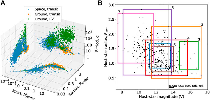
FIGURE 1. (A) Confirmed exoplanets (NASA, 2022) in the mass–radius–period planes depending on the discovery locale (space and ground-based) and on the detection method (transit, RV). For exoplanets with unknown mass or radius, they were calculated using the mass-radius model dependence. (B) Working areas in the host stars’ magnitude–radius plane for seven ground-based telescopes that detect exoplanets using the transit method (shown by dots, 347 out of 386): 1.0.1 m Schmidt telescope, 2.0.18 m Takahashi Epsilon Astrograph, 3.1.3 m Warsaw University telescope, 4.0.2 m telescope, 5.0.2 m Canon, 6.0.4 m Canon, and 7.0.08 m Mamiya 645. Also shown is the minimum limiting magnitude of the considered stars (13.5^m) for data that were obtained with the 0.5-m SAO RAS robotic telescope and are discussed in this article; the maximum limit (19.5^m) is not shown.

Ground-based observations are weighed down by the Earth’s atmosphere which produces star scintillation and variation of seeing and the duty cycle of observations. The wavefront perturbations of stellar light passing through the atmosphere reduce the signal-to-noise ratio, which limits photometric precision and the minimum brightness dimming that can be registered. The brighter the star, the greater is the signal-to-noise ratio, but the decrease in brightness during a transit will be less significant. Therefore, exoplanets near the stars with magnitudes m = 10 − −14^m are mainly detected (300 out of 386) by the transit method in ground-based surveys (Figure 1B). The daily rotation and annual motion of the Earth determine the possibility of observing a given section of the sky from a given observation point. Therefore, the transit of an exoplanet may occur at those moments of time when it cannot be observed, several times in a row, although the technical capabilities make it possible to register the observed decrease in brightness. For reliable detection of exoplanets, one must observe at least several transit events that occur with a period equal to the exoplanet orbital period (for example, it takes several years or more to detect planets at a distance of more than 1 AU from a Sun-like star).

Thus, for the detection of exoplanets by the transit method in ground-based surveys, it is specifically important to increase the number of observed stars and the observation time. For these purposes, it is relevant to use robotic telescopes that regularly perform long-term routine observations of a certain part of the sky (to increase the observation time) or different parts of the sky (to increase the number of stars). The use of a group of such telescopes makes it possible to achieve both the goals.

A group of robotic telescopes is currently being developed at SAO RAS with the aim of detecting exoplanets by the transit method and conducting additional observations of the already known exoplanets. Currently, one such telescope is under operation, automatically observing two regions of the sky since the summer of 2020, each for 6 months. We have developed a piece of software to perform photometric analysis and to search for transit events in the light curves of the stars. In this article, we present the analysis and primary results of processing the first data set obtained in the last third of 2020.

The aim of this work was to examine the obtained data for suitability for the search of exoplanets. To that end, it was necessary to go through all the stages of image processing, determine the problems that arise in the process of data processing, and evaluate the possibility of using algorithms to search for transit events in the light curves. Section 2.2 is devoted to the description of the observations and the quality of the obtained data. Section 2 briefly describes the stages of the developed pipeline and also discusses the problems that arise when working with the data. The primary results of the search for exoplanet candidates are presented in Section 3, which also presents the light curves for some of the observed variable stars. A discussion of the five detected candidates and the prospects of our exoplanet survey are presented in Section 4.

2 Data and Method

2.1 Robotic Telescope Array

The “Astrosib” (Novosibirsk, Russia) RC-500 telescopes with a 0.5-m hyperbolic main mirror were installed on the fast tracking “10 Micron GM 4000” high precision equatorial mounts. In the primary focus, each unit was equipped with an FLI Proline PL16801 front illuminated CCD camera with a 9 μm pixel size. The Baader Planetarium AllSky 4.5-m dome with a weather forecast meteo station and a 4.5-m Astrosib AllSky dome were used as shelters. The FLI CCD camera, FLI Atlas focuser, and FLI five-position motorized 50-mm filter wheel were operated by an industrial PC which collects the raw data and provides remote access.

The cloud and humidity sensors automatically send the telescope into its parking position and signal for the dome to close. The twilight sky flat-field correction frames have been obtained since February 2021. Bias and dark calibration frames are collected daily.

2.2 Observations

From 25 August 2020 to 21 January 2021, surveys were carried out for 84 nights (Figure 2A). Of these, 56 turned out to be suitable for light curve analysis; they are colored in Figure 2A. The white dwarf WD0009 + 501 with a well-known 8-h period and 5 mmag amplitude variations was chosen as the central object in the frame (Valeev et al., 2015). The 2.45 × 1.56° (RA x DEC) field of view around this object has good visibility conditions in the autumn.

FIGURE 2

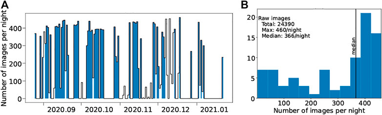
FIGURE 2. Statistics on the number of images per night: (A) distribution by time with the colored columns marking the nights with successfully performed photometry and (B) distribution by number.

Observations were carried out with an exposure of 60 s and with a period of 80–100 s in the V filter of the Johnson system. The image scale was 1.34^″/pixel. Each night, 2 to 460 images were taken; the median value was 366. The total number of images is 24,390 (Figure 2B). In addition, 10 dark and 10 bias frames were made for each night. No flat-field frames were taken.

2.3 Data Processing

The image processing is implemented in Python scripts combined into one bash-script. It can be divided into two independent parts (Figure 3): photometry–automatically obtaining light curves from images and light curve analysis–searching for dimming in the light curves.

FIGURE 3

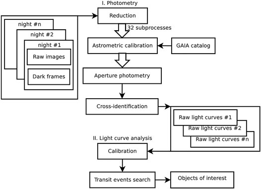
FIGURE 3. Flowchart of the data processing algorithm for detecting exoplanets using the transit method.

A catalog of stars in the considered field was prepared in advance, according to the data on the GAIA space telescope [Prusti et al. (2016); Brown et al. (2021)]: ID, coordinates (ra, dec), magnitude. This catalog contains 39,978 stars with magnitudes m ∈ [13.5,19.5]^m.

2.3.1 Photometry

The entire field was divided into nine overlapping parts: central (2500 × 2500 pix), two sides (820 × 2500 pix), top and bottom (2500 × 820 pix), and four corners (1000 × 1000 pix). For each of the nine parts of the frame, the processing is carried out sequentially for each night, which takes up to 5 min of machine time (CPU frequency 2.2 GHz). Obtaining light curves for one part of the frame for all nights takes up to 2 to 4 h. Reduction, astrometry calibration, and aperture photometry are carried out in a multiprocessing mode, which makes it possible to process 32 images simultaneously at these stages.

The first stage of the pipeline is to create a configuration file based on the parameters entered by the user. After that, a calibration file is prepared. A total of 10 dark frames are combined, and the resulting dark frame is subtracted from the images taken at night. Further, using the astrometry.net package (Lang et al., 2009), the images are calibrated to the celestial coordinate system, and the coefficients of the transition matrix from the rectangular coordinates of the image x, y to astronomical equatorial coordinates ra, dec are determined. Reduction and astrometry calibration are carried out using the CCDpack package (Warren-Smith et al., 2014).

The next step is aperture photometry using the SExtractor package (Bertin and Arnouts, 1999) in eight apertures with a diameter of 4–12 pixels. The PSF of stars falls within this range under various weather conditions (an example is shown in Figure 4). For the identification of stars, the previously prepared GAIA catalog with an association radius of 5 pixels is used. In the resulting table, each star from the catalog identified by the source in the image is assigned an instrumental magnitude for each aperture.

FIGURE 4

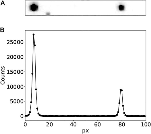
FIGURE 4. Example with two stars in the image after reduction (A) and their projection onto one axis, where each point corresponds to the counts in a pixel (B).

Furthermore, the obtained tables for each image taken at night are combined into a single catalog, in which instrumental magnitudes in eight apertures for the entire night are assigned to each identified star. Thus, as a result of performing the described steps, the light curves of the stars from the input catalog are obtained from raw images for each night. Figure 5A shows a magnitude distribution example for the stars, according to the catalog derived from photometry. For some stars with magnitudes of m = 14^m, the standard deviation reaches minimum values up to 0.005^m (Figure 5B).

FIGURE 5

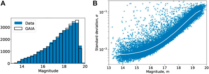
FIGURE 5. Photometry statistics for one night: (A) magnitude distribution compared to the GAIA catalog (Prusti et al. (2016); Brown et al. (2021)) and (B) standard deviation versus magnitude, with the median dependence shown by the white curve.

To select the operating range of magnitudes, we first analyzed the dependence of magnitude, according to the GAIA catalog, on the number of counts on the CCD array. Then, 13.5^m was taken as the lower limit, and 19.5^m was taken as the upper limit. In this range, there are no stars with saturated pixels or those whose signal levels are comparable with the noise levels.

2.3.2 Light Curve Analysis

The light curves obtained for each night are combined into one for all nights. After that, they are calibrated. Stars are selected as standard stars if they satisfy the following conditions: 1) they are identified on all nights, 2) their magnitudes are less than 15.5, and 3) they are in the same part of the frame as the target star. The light curves for several standard stars are shown in Figure 6.

FIGURE 6

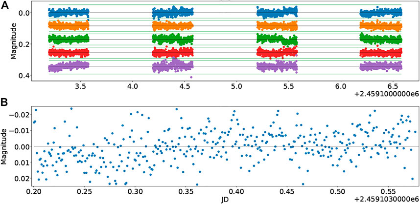
FIGURE 6. Light curve examples for four stars with m ≈ 15.5^m: (A) for 4 nights, with a ±0.05^m zone shown for each star, and (B) for the first star on the first night.

The last step is to search for transit events in the light curves using the BLS (box least squares) method (Kovacs et al., 2002). In this method, the phase folded light curve is approximated by a two-level model: one level (high) before and after the transit and another level (low) during the transit. The function changes instantly at the beginning and at the end of the transit and is similar in shape to a box. The idea of the method is to calculate statistics depending on the differences between the model and the available data. The larger the statistic, the smaller is the residual. For each trial period, the best combination of transit duration and transit start time is determined, which corresponds to the maximum value of the statistics. Thus, a periodogram is constructed, and the dependence of this statistic is on the trial period. On the periodogram, a star with a light curve that exhibits a transit event has a global maximum, which differs significantly from the rest of the local maxima. For each star, a periodogram is plotted for the light curves constructed using five standard stars. The threshold value at which the flag is triggered is set. For most interesting objects, the flag is triggered twice or more. After that, the light curves of the selected objects are viewed individually to decide whether to consider the star as an object of interest.

3 Results

As a result of applying the algorithm to the obtained data (Section 2), five interesting objects were found (named SOI–SAO RAS objects of interest). Their light curves and parameters are shown in Figure 7 and Table 1, respectively.

FIGURE 7

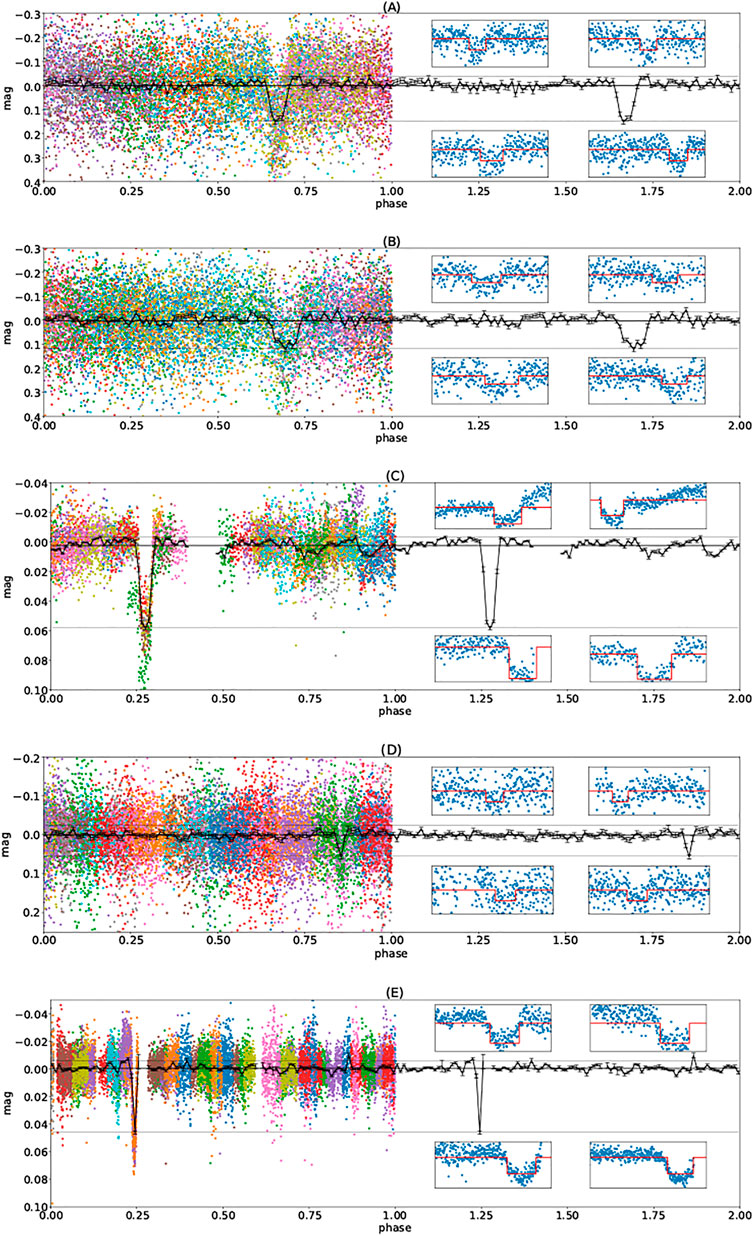
FIGURE 7. Folded light curves of five objects of interest and binned averaged curves (main panels). Points from different periods are shown in different colors. The horizontal lines show the minimum, maximum, and median values. The four small panels show examples of individual transit events with the model found by the BLS method (see their parameters in Table 1).

TABLE 1

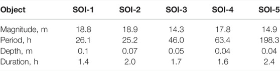
TABLE 1. Objects of interest and transit event parameters.

As a result of the deviation-magnitude relation analysis (Figure 5B), as well as in the process of searching for exoplanets, more than 90 variable stars were found; the light curves for 12 of them are shown in Figure 8. A detailed description of the selection criteria for stars in multiple systems or stars with exoplanet candidates will be updated in the next study. The validation of their binary nature (multiplicity) using additional spectral data from the 6-m BTA telescope has just started.

FIGURE 8

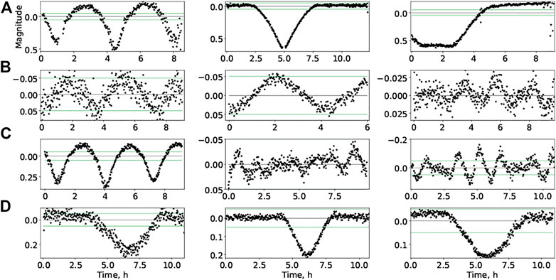
FIGURE 8. Light curves of variable stars: (A) with large amplitudes (Δm > 0.5^m), (B) with small amplitudes (Δm < = 0.1^m), (C) with short periods (P < 4^h), and (D) with a shape similar to a transit event. The horizontal lines show the ±0.05^m zone.

4 Discussion

We have shown in the practice that exoplanet candidates can be found from the obtained data. The dimming in the objects of interest is in the range of δm ≈ 0.04 … 0.1^m, which corresponds to a transit of a 1–2 Jupiter radius exoplanet across the disk of a star of solar radius or less (Figure 9A). They have an orbital period of 1–8 days, corresponding to a planet orbiting close to the host-star, with the semi-major axis less than 0.08 AU (Figure 9B). These estimates indicate that hot Jupiter or, possibly, hot Neptune are the targets of our search for exoplanet candidates. After processing the data in this sky area for the second half of 2021, we have planned to search for exoplanets in wider orbits with periods of up to several months. The transit durations of all the SOI with determined periods are less than the corresponding maximum value; they passed this initial test successfully. SOI-2 remains mostly unclear. The odd and even minima in the light curve of SOI-2 differ. Furthermore, based on the detected objects, we can improve the algorithm by refining the criterion for selecting transit events.

FIGURE 9

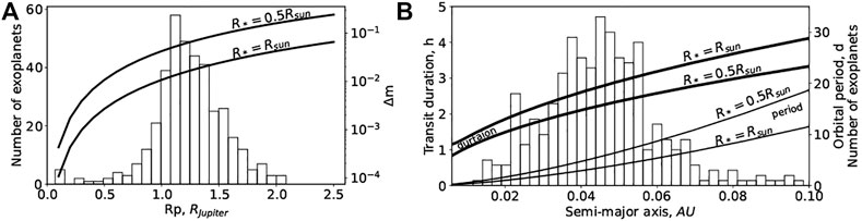
FIGURE 9. Maximum brightness dimming of the host star during a transit event Δm versus the exoplanet radius ((A), right axis) and (B) transit duration (left axis and bold lines) and orbital period (right axis and thin lines) versus the semi-major axis of the exoplanet orbit for the stars of solar radius and those two times smaller. Also shown are the histograms of the distribution of confirmed transiting exoplanets (NASA, 2022) detected by ground-based facilities by the exoplanet radius ((A), left axis) and by the semi-major axis of their orbits ((B), right axis).

The detected objects must undergo further validation. To that end, we have planned to carry out additional photometric and spectral measurements. The light curves in different filters and the radial velocity (RV) amplitudes of the stars will allow us to reject the double star hypothesis. The shape of the residual between the light curves in different filters during the transit of an exoplanet differs from the shape for an eclipsing binary star with different spectral type components. The RV amplitude determines the minimum mass of the component that produces dimming. On one hand, most ground-based surveys observe brighter stars, so our observations in the range of m ∈ [13.5,19.5]^m can be productive. However, the necessary validation of faint objects by the RV method is more difficult. There is also less information about faint stars, so modeling transit events for validation purposes is more uncertain. Therefore, it is possible that in the future, this range will be shifted toward brighter stars.

The disadvantage of the existing pipeline is the different orientation of raw images, which complicates the last step of creating the light curve, when the star’s light curves converge into one for all nights. Therefore, in the future, we have planned to transform each image at the first stage, bringing all the images to the same orientation. In addition, it is possible to speed up the process by forming packages of consecutive images to reduce the time of astrometric calibration. At the light curve analysis stage, detrending needs to be added.

Currently, the data have been processed only for the last third of 2020, but the same sky field was observed in 2021; 2021 data are also available for another field. After processing these data and improving the algorithm, the pipeline will be introduced into the observing process. Processing will be carried out immediately after the observation.

Data Availability Statement

The raw data supporting the conclusion of this article will be made available by the authors, without undue reservation.

Author Contributions

OY and AV wrote the manuscript and performed data processing. GV, VS, and VV managed the process of facility design and construction. AT and OK stated the problem of exoplanetary research. VA, GM, EE, and TF performed the observation. EE and TF domed and mounted the software development. AP and SB maintained instrumental and technical solutions. TB performed software testing and database engineering. GG, GB, SF, and IR proposed the grant for AstroM funding. SB designed the solution at the first stage; SB died in 2019.

Funding

The study was supported by the Government and the Ministry of Education and Science of Russia (Grant No.075-15-2020-780 (N13.1902.21.0039)). AV acknowledges the star multiplicity advocation algorithm development, which was supported by the Russian Science Foundation G rant No 19-72-10023.

Conflict of Interest

AP and SB were employed by the Research Corporation “Precision Systems and Instruments”.

The remaining authors declare that the research was conducted in the absence of any commercial or financial relationships that could be construed as a potential conflict of interest.

Publisher’s Note

All claims expressed in this article are solely those of the authors and do not necessarily represent those of their affiliated organizations, or those of the publisher, the editors, and the reviewers. Any product that may be evaluated in this article, or claim that may be made by its manufacturer, is not guaranteed or endorsed by the publisher.

Acknowledgments

In this study, we used the NASA Exoplanet Archive, which is operated by the California Institute of Technology, under contract with the National Aeronautics and Space Administration under the Exoplanet Exploration Program. This work has made use of data from the European Space Agency (ESA), mission Gaia (https://www.cosmos.esa.int/gaia), processed by the Gaia Data Processing and Analysis Consortium (DPAC, https://www.cosmos.esa.int/web/gaia/dpac/consortium). Funding for the DPAC has been provided by national institutions, in particular the institutions participating in the Gaia Multilateral Agreement.

References

Auvergne, M., Bodin, P., Boisnard, L., Buey, J.-T., Chaintreuil, S., and Team, C. (2009). The CoRoT Satellite in Flight : Description and Performance. Astronomy Astrophysics 506, 411. doi:10.1051/0004-6361/200810860

CrossRef Full Text | Google Scholar

Bakos, G., Noyes, R. W., Kovács, G., Stanek, K. Z., Sasselov, D. D., and Domsa, I. (2004). Wide‐Field Millimagnitude Photometry with the HAT: A Tool for Extrasolar Planet Detection. Publ. Astron Soc. Pac 116, 266–000277. doi:10.1086/382735

CrossRef Full Text | Google Scholar

Bertin, E., and Arnouts, S. (1996). SExtractor: Software for Source Extraction. Astron. Astrophys. Suppl. Ser. 117, 393–404. doi:10.1051/aas:1996164

CrossRef Full Text | Google Scholar

Borucki, W. J. (2016). KEPLERMission: Development and Overview. Rep. Prog. Phys. 79, 036901. doi:10.1088/0034-4885/79/3/036901

PubMed Abstract | CrossRef Full Text | Google Scholar

Brown, A., Vallenari, A., Prusti, T., and de Bruijne, J. (2021). Gaia Early Data Release 3. Summary of the Contents and Survey Properties. Astronomy Astrophysics 650, 7. doi:10.1051/0004-6361/202039657e

CrossRef Full Text | Google Scholar

[Dataset] NASA (2022). NASA Exoplanet Archive. Washington, D.C., USA: NASA. doi:10.26133/NEA12

CrossRef Full Text | Google Scholar

Deeg, H. J., and Alonso, R. (2018). Transit Photometry as an Exoplanet Discovery Method. Handb. Exopl. 2018, 633–657. doi:10.1007/978-3-319-55333-7_117

CrossRef Full Text | Google Scholar

Kovács, G., Zucker, S., and Mazeh, T. (2002). A Box-Fitting Algorithm in the Search for Periodic Transits. Astronomy Astrophysics 391, 369–377. doi:10.1051/0004-6361:20020802

CrossRef Full Text | Google Scholar

Lang, D., Hogg, D. W., Mierle, K., Blanton, M., and Roweis, S. (2010). Astrometry.net: Blind Astrometric Calibration of Arbitrary Astronomical Images. Astronomical J. 139, 1782–1800. doi:10.1088/0004-6256/139/5/1782

CrossRef Full Text | Google Scholar

Pollacco, D., Skillen, I., Cameron, A., Christian, D., Irwin, J., Lister, T., et al. (2006). The WASP Project and SuperWASP Camera. Astrophys. Space Sci. 304, 253–255. doi:10.1007/s10509-006-9124-x

CrossRef Full Text | Google Scholar

Prusti, T., de Bruijne, J., Brown, A., Vallenari, A., Babusiaux, C., Bailer-Jones, C., et al. (2016). The Gaia Mission. Astronomy Astrophysics 595, 36. doi:10.1051/0004-6361/201629272

CrossRef Full Text | Google Scholar

Ricker, G., Winn, J., Vanderspek, R., Berta-Thompson, Z., Levine, A., Seager, S., et al. (2015). Transiting Exoplanet Survey Satellite (TESS). J. Astronomical Telesc. Instrum. Syst. 1 (1), 014003. doi:10.1117/1.JATIS.1.1.014003

CrossRef Full Text | Google Scholar

Rosenthal, L. J., Fulton, B. J., Hirsch, L. A., Isaacson, H. T., Howard, A. W., Dedrick, C. M., et al. (2021). The California Legacy Survey. I. A Catalog of 178 Planets from Precision Radial Velocity Monitoring of 719 Nearby Stars over Three Decades. ApJS 255, 8. doi:10.3847/1538-4365/abe23c

CrossRef Full Text | Google Scholar

Valeev, A. F., Antonyuk, K. A., Pit, N. V., Solovyev, V. Y., Burlakova, T. E., Moskvitin, A. S., et al. (2015). Detection of Regular Low-Amplitude Photometric Variability of the Magnetic Dwarf WD0009+501. On the Possibility of Photometric Investigation of Exoplanets on the Basis of 1-meter Class Telescopes of the Special and Crimean Astrophysical Observatories. Astrophys. Bull. 70, 318–327. doi:10.1134/S1990341315030104

CrossRef Full Text | Google Scholar

Warren-Smith, R., Draper, P., Taylor, M., and Allan, A. (2014). CCDPACK: CCD Data Reduction Package. Astrophys. Source Code Libr. 2018.

Google Scholar

Wright, J. T. (2018). Radial Velocities as an Exoplanet Discovery Method. Handb. Exopl. 2017, 619–631. doi:10.1007/978-3-319-55333-7_4

CrossRef Full Text | Google Scholar