Pipeline for the Antarctic Survey Telescope 3-3 in Yaoan, Yunnan

AST3-3 is the third robotic facility of the Antarctic Survey Telescopes (AST3) for transient surveys to be deployed at Dome A, Antarctica. Due to the current pandemic, the telescope has been currently deployed at the Yaoan Observation Station in China, starting the commissioning observation and a transient survey. This article presented a fully automatic data processing system for AST3-3 observations. The transient detection pipeline uses state-of-the-art image subtraction techniques optimized for GPU devices. Image reduction and transient photometry are accelerated by concurrent task methods. Our Python-based system allows for transient detection from wide-field data in a real-time and accurate way. A ResNet-based rotational-invariant neural network was employed to classify the transient candidates. As a result, the system enables the auto-generation of transients and their light curves.

1 Introduction

The Antarctic Survey Telescope (AST) 3-3 is the third telescope planned for time-domain surveys at Dome A, Antarctica. Before shipping to Dome A, it was placed in the Yaoan observation station of the Purple Mountain Observatory for transient searching in the next several years. Yuan et al. (2015) have described an overview schedule and designation for AST3 series telescopes. The AST3 series includes three large field-of-view (FoV) and high photometric precision 50/68 cm Schmidt telescopes (Li et al., 2019). The AST3-3 is designed for time-domain surveys in the K-band to search for transients in infrared at Dome A. Due to the underdevelopment of infrared instruments of AST3-3, we temporarily used a CMOS camera (QHY411 with Sony IMX411 sensor) with a g-band filter for this commissioning survey instead. This camera has an effective image area of 54 mm × 40 mm and a pixel array of 14304 × 10748 with exposure times ranging from 20 μs to 1 h. With the CMOS camera, the FoV is 1.65° × 1.23°, the pixel scale is 0.41 arcsec, and the typical magnitude limit is 20 ∼ 20.5 in the g-band for 60 s exposure images.

In the Yaoan observation station, we used the fully automatic AST3-3 telescope for a time-domain sky survey and follow-up observation. We have constructed an observation scheme for the follow-up observation of transients, according to the notices from Gamma-ray Coordinates Network (Barthelmy, 2008). The summary of our observation system and hardware, the survey and target-of-opportunity strategy, and the early science results will be presented in a forthcoming publication (Sun et al. in prep.).

This article presented a detailed overview of the AST3-3 data pipeline system. We have designed an automatic pipeline system containing data reductions, transient detection, and a convolutional neural network (CNN) framework for transient classifications. The data reduction pipeline includes instrumental correction, astrometry, photometry calibration, and image data qualification estimations. The transient detection pipeline consists of the alignments of images, image subtractions, and source detection on subtracted images.

The image subtraction algorithm automatically matches the point spread function (PSF) and photometric scaling between the reference and science images. In particular, one prevalent approach is the algorithm initially proposed by Alard and Lupton (1998) and further developed by a series of works (Alard, 2000; Bramich, 2008; Becker et al., 2012; Bramich et al., 2013; Hu et al., 2021). This technique has been extensively used in the transient detection pipelines (Zhang et al., 2015; Andreoni et al., 2017; Masci et al., 2019; Zhang et al., 2020; Brennan and Fraser, 2022). In the last decade, it has played an important role in many successful time-domain survey programs, including intermediate Palomar Transient Factory (Cao et al., 2016), Dark Energy Survey (Morganson et al., 2018), and Panoramic Survey Telescope And Rapid Response System-1 (PS1 hereafter, Price and Magnier, 2019).

Time-domain surveys are demanded to find transients as fast as possible, but many bogus candidates are detected from the image subtraction results. The human workload can be greatly reduced by the classifier methods such as machine learning and deep learning (Gómez et al., 2020; Yin et al., 2021). Random forest and some other machine learning methods previously attempted to solve the classification problem (Goldstein et al., 2015). We have applied a CNN framework to the estimation of the image qualification and candidate selections after transient extraction in this work. The CNN found optimal results with backpropagation (Rumelhart et al., 1986), and its accuracy has approached the human level in some classification and identifying tasks (Lecun et al., 2015). Similar to some sophisticated neural networks, these CNN models can naturally integrate features from different levels and classify them in end-to-end multilayer neural networks. Dieleman et al. (2015) introduced the first rotation invariant CNN to classify galaxies by considering the inclination of the object in the classification. The approach using the rotation-invariant CNN soon makes its way into the transient survey programs, e.g., The High cadence Transient Survey (HiTS; Förster et al., 2016) aimed at searching transients with short timescales. In the transient detection procedure of the HiTS, Cabrera-Vives et al. (2017) used the rotation-invariant CNN to classify the real transient candidates and the fake candidates from the image subtractions. Jia et al. (2019) modified the rotation-invariant CNN by adding the long short-term memory network (Hochreiter and Schmidhuber, 1997) to enhance the performance in the satellite trail identifications. The alert classification system for the Zwicky Transient Facility survey also uses the updated rotation-invariant CNN (Carrasco-Davis et al., 2021). The previous CNN structures for classification used superficial layers for feature extraction, and residual learning frameworks have been introduced in He et al. (2015) to avoid the loss of too much information and the difficulty of deeper CNN.

In Section 2, we described the data reduction pipeline and the qualification evaluation methods for image data. The transient detection pipeline for AST3-3 is presented in Section 3. Section 4 describes the CNN structure and training for classifying transient candidates and their performance. We showed the conclusions in Section 5.

2 Data Reduction Pipeline

The data reduction pipeline aims at reducing the instrumental effects on the observational image to create the scientific image and apply the basic calibration information. This pipeline stage contains a group of subroutines for instrumental correction, astrometry, and photometry calibration. We also added a group of methods for evaluating the quality of images. The entire flow for the single-frame image processing is shown in Figure 1.

FIGURE 1

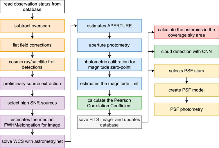
FIGURE 1. Flow of the single-frame image processing for AST3-3.

2.1 Instrumental Correction

The instrumental calibrations include overscan area removal and bias correction, flat-field correction, bad pixels, and cosmic-ray detection. The CMOS sensor of the camera on AST3-3 provides a 14304 × 10748-pixel image array including a narrow overscan area of 50 lines. which contains the data for bias corrections. We used the median of the overscan area for each line as a bias field value similar to the CCDPROC method (Craig et al., 2015) and produced an image array of 14206 × 10654 pixels. The bias correction effectively removes the background boost from the offset value in the camera settings.

The AST3-3 telescope observes about 80 flat field images at a half-full maximum of the pixel capacity of near 30000 ADUs every observable twilight. The flat field image was constructed with the sigma-clipped median method like IRAF (National Optical Astronomy Observatories, 1999) and applied to the observation images. The image also contains the cosmic ray defects on the detector, and we added the L.A.Cosmic package for the cosmic ray identification with the Laplacian edge detection method (van Dokkum, 2001). A growing number of satellites plot trails on images that shall be added to the mask image. The pipeline uses the MaxiMask and MaxiTrack methods for star trail detections (Paillassa et al., 2020).

2.2 Astrometry Calibration

The pipeline for astrometry calibration solves the solution for the world coordinate system (WCS, Calabretta and Greisen, 2000) and fits the WCS distortion parameters. The astrometry solution and the estimation of full-width half-maximum (FWHM) for images require source detection, and we optimized the sequence. The FWHM is a critical parameter in describing how the turbulence of the atmosphere and the properties of the optical system affect the observations of point sources. The pipeline uses the SExtractor (Bertin and Arnouts, 1996) at first to detect sources on the image and measure basic parameters of stars with the automatic aperture photometry method. The preliminary photometry catalog results contain some bad sources, and we cleaned out the bad detection with the following restrictions:

• The neighboring, blended, saturated, or corrupted stars were excluded by removing the sources with FLAGS larger than zero.

• The sources with the automatic aperture flux parameter FLUX_AUTO that is not zero and the ratio of FLUX_AUTO and FLUXERR_AUTO larger than 20 were excluded.

• The isophotal and automatic aperture result parameter MAG_BEST lower than 99 was selected to exclude the bad magnitude fitting.

• The outlier of FWHM_IMAGE and elongations of sources were excluded by the sigma clip method with the 3σ threshold.

• The catalog was sorted by the star-galaxy classification CLASS_STAR, and the last 20% of the catalog was removed.

The remaining catalog contained the most of detected point sources. We used the median of the FWHM_IMAGE for sources in the remaining catalog as the FWHM of the image. The pipeline calls the solve-field program in Astrometry.net (Lang et al., 2010) to fit the WCS for their flexible local index files built from the Gaia Data Release 2 (Gaia Collaboration et al., 2018). We provided the X, Y, MAG_BEST list for point sources, the pointing RA and DEC, the search radius, and the estimated pixel scale for the solve-field program to speed up the searching and fitting procedure.

AST3-3 has a large FoV of 1.65° × 1.23°, which requires distortion corrections in the WCS. The pipeline also calculates the WCS with a fourth-order simple imaging polynomial (SIP, Shupe, et al., 2005) distortion for the accuracy of the coordinates. The mean solving time for ordinary observation is approximately 1.7–2 s for a catalog generated by the SExtractor.

2.3 Photometry

The pipeline extracts sources and estimates their flux and magnitudes on the image. We have applied the aperture photometry and PSF photometry methods in the pipeline. The aperture for aperture photometry is determined with Equation 1. A_IMAGE is the semimajor axis value in the catalog what matches the selection criteria in Section 2.2 and the default value C = 6.0 as derived in Sokolovsky and Lebedev (2018),

$\text{Aper}=C\times \text{median}\left(\text{A}\text{\_}\text{IMAGE}\right).(1)$

Aperture photometry is performed by the SExtractor with the DETECT_THRESH of 2σ and the estimated aperture. The pipeline cleans the catalog from aperture photometry with the same distilling criteria described in Section 2.2. The estimation of the magnitude zero-point calculates the difference between aperture photometry and a reference catalog. We have selected PS1 (Chambers and Pan-STARRS Team, 2017) as the reference catalog for magnitude calibration for its sky coverage and much better magnitude limits. We used a χ² minimization method introduced in the PHOTOMETRYPIPELINE (Mommert, 2017) to generate the magnitude zero-point as Equation 2:

${\chi }^2=\sum _i^N\frac{{\left(m_{zp}-{\chi }_i\right)}^2}{{\sigma }_{\chi ,i}^2}.(2)$

In Equation 2, the i-th parameter χ_i is the difference between the aperture magnitude and the g magnitude in PS1 for the i-th source in the catalog for all N-matched sources. The magnitude zero-point m_zp is determined by minimizing χ² with an iterative process to reject outlier samples.

The magnitude zero-point calibration has some residual due to the spatial variation in the atmospheric extinction across the large FOV. We used a quadratic form to fit the offsets between the reference catalog and the zero-point calibrated aperture magnitudes. The 2D polynomial formula to fit the residuals is shown in Equation 3, introduced in Irwin et al. (2007):

$\mathrm{\Delta }m\left(x,y\right)=c_0+c_{1}x+c_{2}y+c_{3}xy+c_4{x}^2+c_5{y}^2.(3)$

Δm is the zero-point offset for a star, and c_i are the polynomial coefficients for the equation. Given that the background noise dominates the flux uncertainty of the faintest sources, the pipeline estimates the limiting magnitude based on the sky background with the method of Kashyap et al. (2010) with the root mean square of background by the Python library SEP (Barbary, 2016).

PSF photometry requires a group of well-selected stars for profile fitting. We selected the sources in the aperture photometry catalog with the same criteria in Section 2.2 but limited the restriction of FWHM_IMAGE and ELONGATION to 1σ to keep the best ones.

The pipeline feeds the selected catalog to PSFEx (Bertin, 2013) to generate a position-dependent variation PSF model. The SExtractor accomplishes the PSF photometry with the result of PSFEx. It takes a relatively long time for PSF fitting and model fitting in PSF photometry. This part works in the background after the single-frame image process.

2.4 Data Quality Inspection

This subsection introduces the image quality inspection method, which estimates how the cloud affects the observation image. The magnitude limit is an excellent parameter for the qualification of an image. For a large FoV telescope, the image extinction and airmass may vary across the FoV of the instrument, especially at lower altitudes. The magnitude limit may also vary across the FoV of the instrument, producing spatial variations of the limiting magnitudes. In ideal observation conditions, we suppose that the extinction is consistent everywhere in the image, which causes all-stars to have the same magnitude difference between the machine magnitude and reference catalog. Small clouds also influence the photometry results due to their discontinuous extinction to the nearby image parts. In the affected parts of the image, the flux of stars and galaxies would be reduced by clouds more than in other regions. In addition to the effects of clouds and extinction, incorrect WCS fits resulting in false star catalog matches can seriously affect the magnitude corrections.

Based on the corrected aperture magnitudes and reference magnitudes being equal within the margin of error, we calculated the correlation between them. The measurement uses the Pearson correlation coefficient (also called Pearson’s r, PCC hereafter, Pearson and Galton, 1895). The pipeline also selects stars that match the criteria, as described in Section 2.2, and calculates the PCC as Equation 4:

$r=\frac{\sum \left(\left(m_a-\overline{m_a}\right)\left(m_g-\overline{m_g}\right)\right)}{\sqrt{\sum {\left(m_a-\overline{m_a}\right)}^2\sum {\left(m_g-\overline{m_g}\right)}^2}}.(4)$

Equation 4 gives the expression of PCC, where m_a means the aperture photometry magnitude, and m_g is the g-band magnitude in PS1. For a completely ideal situation, the value of PCC becomes 1. For a typical AST3-3 image, the PCC value should be larger than 0.98 to avoid the influence of the clouds. When using PCC to estimate the image quality, we noticed that the uniform thin clouds do not influence the PCC in some images in a very significant way. Figure 2 shows a typical image of the good PCC with an obvious cloud on the image at an altitude of 53°.

FIGURE 2

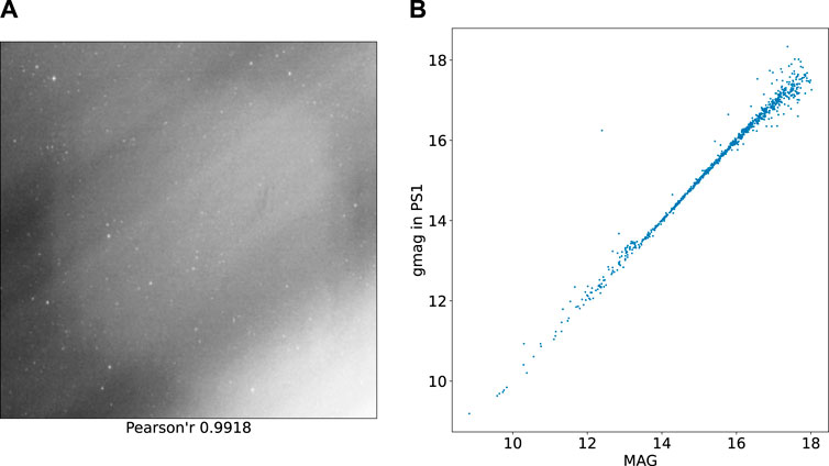
FIGURE 2. (A) shows the thumbnails of an AST3-3 image with obvious cloud effects. (B) is a scatter plot of the calibrated aperture photometry magnitude and g-mag in PS1.

The discontinuous extinction would cause errors in flux calibrations in the image subtraction process for transient detection. As we can see the cloud from the thumbnails in the left panel of Figure 2, we could screen out the images with cloud effects manually. The pipeline creates thumbnails with the Zscale (National Optical Astronomy Observatories, 1999) adjustment and normalization method in Astropy (Greenfield et al., 2013) to downscale it to an image size of 256 × 256 pixels.

Our manually checked results showed that the cloud effects were still visible in the thumbnails. Thus, the cloud image classification for images is a simple classification problem that could be solved with the CNN method.

Consequently, we converted the cloud image classification into a simple image classification problem. We attempted to check for clouds in the images using the 18-layer residual neural nets (ResNet-18, He et al., 2015), as shown in Table 1. ResNet-18 is the simplest structure of residual neural networks, allowing a deeper network with faster convergence and easier optimization. We have chosen the original ResNet-18 structure as there are no vast data. The AST3-3 data are monochrome, which means we have only one channel of data to the input layer of the CNN. We have modified the input layer to the input channel of 1, output channel of 64, kernel size of 7 × 7, and stride of 1 to match the thumbnail data and the second layer. Three fully connected layers construct the classifier for the features extracted by ResNet-18. In the classifier part, we selected the default rectified linear units (ReLU, Nair, and Hinton, 2010) function as the formula of max (0, x) as the activation function.

TABLE 1

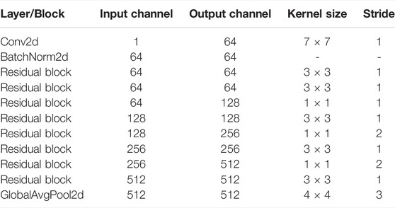
TABLE 1. Residual neural network structure with the residual block.

The CNN training data set contains 1000 clear images and 1000 cloudy images as a balanced dataset. To avoid overfitting in the CNN training, we used dropout to 0.5 in the classifier layers. We have selected 20% of the balanced data set as the test set for validation during the training of ResNet-18. The training uses the optimizer AdamW (Loshchilov and Hutter, 2017) and a scheduler for reducing the learning rate after each training epoch. The CNN-trained result shows accuracy in the test group of 98.35% and a recall rate of 98.28%. CNN’s classification of the thumbnail results is helpful as an indicator for significant cloud effects from our results. In practice, if CNN’s classification of the thumbnail is cloud-affected, the image would be marked in the database and the website. If there is an obvious problem with the result of transient detection, like a massive number of detected candidates with a cloud-affected report, the image would be dropped automatically.

The data reduction pipeline schedules the single-image process independently to each image as a standalone thread concurrently. The approximate average calculation time for the sparse starfield is 17 s per image after the observation. The pipeline also marks the necessary information into the FITS header and updates the database for the following step programs.

2.5 Data Reduction Pipeline Performance

We have estimated the accuracy of the WCS for images by comparing the star position difference between the WCS and the Gaia-DR2 catalog. For each image, we matched the catalog between the aperture photometry result and the Gaia-DR2 catalog and calculated the difference between right ascension and declination for the matched stars. The astrometry standard deviation in the data reduction pipeline is between 100 and 200 mas, as shown in Figure 3.

FIGURE 3

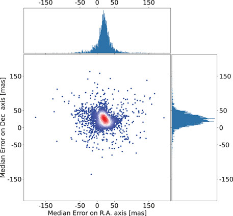
FIGURE 3. Main scatter-plot shows the median deviation distribution of the astrometric error along each axis with respect to the Gaia-DR2 catalog for AST3-3 for stars in three thousand images. The upper and right panel shows the histograms of the distributions for both axes.

The local PSF photometry results have some differences from the Pan-STARRS DR1 catalog due to some noise that should be well-fitted. We selected an example of sky area “0735 + 1300” at an altitude of 75° above the horizon to show the result of PSF photometry fitting and the magnitude zero-point calibration. Figure 4 shows the difference map with density color and the standard deviation trends from the detected bright to dark sources.

FIGURE 4

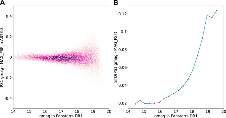
FIGURE 4. (A): Difference between the AST3-3 g-band photometry and PS1 g-mag values. (B): Standard deviation of the binned and sigma clipped difference between the AST3-3 mags and PS1 g-mags.

Figure 5 shows the PCC correlation distribution described in Section 2 since the first light in the Yaoan observation station on 27 March 2021. In all the 60-s exposure images, 98% of them had a PCC value greater than 0.95, and 84% of them had a better PCC value of 0.99.

FIGURE 5

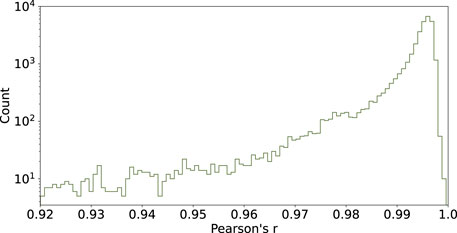
FIGURE 5. PCC value distribution for 33539 images since AST3-3 starts observation in 60-s exposure modes.

3 Transient Detection Pipeline

The transient detection pipeline compares the newly observed science image with the previously observed template image data to find the transients appearing on images. This section builds a fully automatic pipeline for transient searching with the alignment method, image subtractions, and source detection on the different images. We adopted the GPU version of the Saccadic Fast Fourier Transform (SFFT) algorithm (SFFT hereafter, Hu et al., 2021) to perform the image subtraction. The SFFT method is a novel method that presents the least-squares question of image subtraction in the Fourier domain instead of real space. SFFT uses a state-of-the-art δ function basis for kernel decomposition, which enables sheer kernel flexibility and minimal user-adjustable parameters. Given that SFFT can solve the question of image subtraction with fast Fourier transforms, SFFT brings a remarkable computational speed-up of an order of magnitude by leveraging CUDA-enabled GPU acceleration. In real observational data, some sources can be hardly modeled by the image subtraction algorithm, and we should exclude them to avoid the solution of image subtraction being strongly misled. In our work, we used the built-in function in SFFT to pre-select an optimal set of sub-areas for a proper fitting.

For the automatic follow-up observation of some transients, we need a rapid image subtraction process to search the possible transient candidates. AST3-3 science images are 14206 × 10654 pixels in size, with a very sparse star field for high galactic latitude observations. The large data array takes a long time for kernel fitting and convolutions in image subtraction. We built two pipeline systems for transient detection. One focused on the quick analysis of the newly acquired image, especially for target-of-opportunity observations (quick image processing, QIP), and another one aimed at obtaining more reliable detections (deep image processing, DIP). The comparison of the two systems is shown in Table 2. QIP uses the 3 × 3 binned image of size 3552 × 4736 pixels to boost the image alignment and subtractions. The 3 × 3 binned pixel scale increased to 1.23 from 0.41 arcsec per pixel, which increased the sky background noise. The flowchart of the pipeline system is shown in Figure 6.

TABLE 2

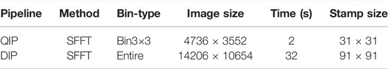
TABLE 2. Processing time for different methods.

FIGURE 6

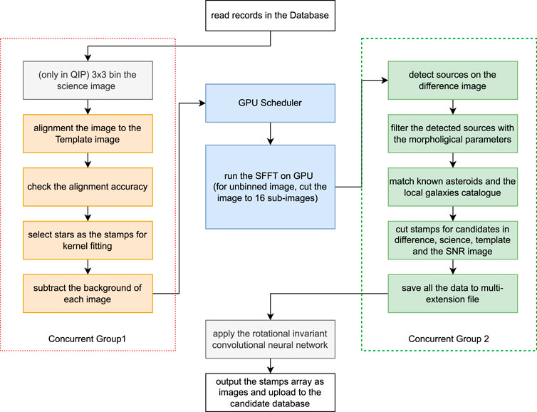
FIGURE 6. This flowchart shows the transient detection pipeline for AST3-3. The pipeline is divided into four components. The left box shows the first concurrent group that contains the preparations for image subtractions. The middle part is the SFFT subtraction procedure, which calls the SFFT functions with a GPU resource scheduler. The right box shows the second concurrent group for candidate detection on the difference images. The bottom part shows the candidate classification and the data exchange of the database.

It is essential to prepare optimal template images to enable transient detections. We chose the earliest acceptable image taken for each sky area with restrictions on image qualities. The magnitude limit for templates should be better than 18.5 magnitudes. The PCC value was greater than 0.98, and there was no apparent cloud structure. The template image is copied directly after the data reduction pipeline result and tagged as the reference in the database. We created the template images for the QIP from the template image by the bin 3 × 3 method. Since the template image for the QIP is a new image, we run the photometry and astrometry on the image with the same method in Section 2. The header of the WCS part of the template image is saved as a separate file to facilitate the SWarp (Bertin, 2010) for the alignment of the science image to the template.

The strategies of each step for the QIP and DIP programs are the same: the resampling and interpolation of images for alignment, the kernel stamp selection, image subtractions, and the source detections on the difference images. As a survey telescope, AST3-3 has a fixed grid for observation. The shift and rotation between two images are tiny for each sky area but exist. Image alignment corrects the positional difference with a transformation matrix between the WCS of the template and science images. We used the SWarp for the resampling procedure with the LANCZOS3 algorithms. For the QIP part, the science image was binned to 3552 × 4736 pixels by scikit-image before resampling.

We performed image subtraction using SFFT for the binned images in QIP and the full-frame images in the DIP branch, respectively. It should be noted that the subtraction tasks are scheduled via the database, and the two branches are triggered concurrently. The resulting difference images are used to detect transient candidates.

The calculations involved in SFFT are carried out using the multiple NVIDIA A100 GPUs equipped on our computing platform. For the QIP case, we performed image subtraction straightforwardly for the 3 × 3 binned images. For the DIP case, we split the large full-frame image into a grid of sub-images with the size of 3072 × 4096 pixels to avoid memory overflow.

The pipeline uses the SExtractor to perform the target search on the different images. We run the SExtractor with aperture photometry and a threshold (DETECT_THRESH) of 2σ for searching the star-like objects on the different images. Some detected negative sources have obvious problems finding stars on the subtracted images. We cleared the bad sources with the following criteria:

• The sources with FWHM_IMAGE lower than one pixel or more extensive than two times the image FWHM were excluded.

• The sources with ELONGATION lower than 0.5 or larger than 6 were excluded.

• The sources with ISOAREA_IMAGE less than four were excluded.

• The sources with FLAGS less than four were excluded.

• The sources near the image edge in 16 pixels were excluded.

After cleaning up, the catalog of different images became the candidate catalog. Extragalactic transients have their host galaxies nearby, and most galaxies are already known. The pipeline cross-matches the candidate catalog with the GLADE catalog (Dalia et al., 2021) with coordinates to obtain some near galaxy transients.

It is easy to detect many asteroids at the Yaoan station due to its latitude. The pipeline calculates the location of asteroids by PyEphem (Rhodes, 2011) with the Minor Planet Center Orbit (MPCORB) Database for each image. It also cross-matches all the candidate catalogs with the local asteroid catalog to exclude the known asteroids.

The transient detection program pipeline ends when the provisional source detection is complete. As the transient detection program could reproduce all the data with the science images, they are retained for only 30–60 days to save storage space. We have built a multi-HDU (Header Data Unit) FITS format regulation to facilitate program error checking to store the data. The primary HDU stores only header information, describing a summary of this image subtraction process results. The other HDUs store the subtracted image, the aligned image, the template image, and the star list of the temporal source candidates through a compressed FITS image (Pence et al., 2009).

The image alignment is handled by SWarp based on the WCS information of the template and science images. The position difference should be near zero for stars on both the template and alignment images to avoid the error occurrence during image subtraction. It is a fast method to check the accuracy of image alignment by examining the position difference between the catalogs from the alignment image and the reference image. Thence, we match the alignment catalog by SExtractor and the reference catalog with the grmatch program in FITSH (Pál, 2012). The position difference is calculated from the position of matched stars in the X and Y planes. Figure 7 shows the median distributions of matched star-position deviations of the DIP and QIP pipelines. The image alignment accuracy of our pipeline is typically less than 0.05 pixels, with a standard deviation of fewer than 0.2 pixels. The QIP has only slightly degraded accuracy due to the pixel scale binned to 1.23 arcsec.

FIGURE 7

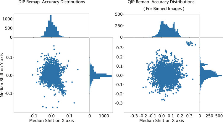
FIGURE 7. Two panels show the standard deviation of the x and y position differences in matched stars between the reference and remapped images. The right panel shows the unbinned images’ remap accuracy, and the left panel shows the remap accuracy for QIP.

The observation of asteroid 1875 is shown in Figure 8 by the time-domain survey and selected by the transient detection pipeline. It is a well-detected example of the pipeline described in this section. The target magnitude is 18.24 in an image with a magnitude limit of 19.9. The target can be seen clearly in the difference image and the pattern of nearby bright stars.

FIGURE 8

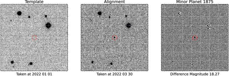
FIGURE 8. Example of the QIP: the detection of minor planet # 1875 at magnitude 18.27. The left panel shows the template image taken on 1 January 2022, and the middle panel shows the remapped image taken on 30 March 2022. The right panel shows the difference images produced by the QIP pipeline.

The performance of QIP and DIP procedures in images is only relevant to their pixel binning properties. As a result, the background and background’s standard deviation increases, decreasing the limiting magnitude of the images in QIP. Since the QIP is only designed for the image with high priority observations, the resources used for QIP are restricted in both GPU time and the threshold of source extraction on the difference image. The QIP finished after the image was taken about 60 s, and the DIP finished after the image observation of about at least 5–10 min due to the GPU time queuing.

4 Candidate Classifications

The AST3-3 telescope is monochromatic in the g-band. It is difficult to distinguish among different types of transient sources with their morphological information in only several images. We divided the detected candidates into two categories: positive and negative candidates. The positive candidates are new point sources or variable sources on the science image. The positive candidates could be any astrophysical origin targets, while the negative candidates mainly originate from residuals and errors of the image subtraction pipelines. In this section, we chose to use the CNN-based approach to filter out the negative candidates from the image subtraction procedures.

4.1 Rotation-Invariant Neural Network

The original rotation-invariant CNN for classifying natural and artificial sources from transient detection pipelines is introduced in Cabrera-Vives et al. (2017) for HiTS as the CNN model named Deep-HiTS. The Deep-HiTS uses the data array by combining difference images, template images, science images, and signal-to-noise ratio images as the stamps to classify the candidates generated from the detection after image subtraction. The original Deep-HiTS network rotates the combination of images to 0, 90, 180, and 270° to feed four independent CNNs for feature extraction. The CNN parts of Deep-HiTS only use a simple seven-layer structure that more complex neural networks can replace.

It is expected that there should be nonlinear activation functions between the layers of the CNN to enhance the performance of multilayer structures. The rectified linear units (ReLU, Nair, and Hinton, 2010) and their modifications are activation functions widely used in recent years. The ReLU function discards all negative values with max (0, x) for the sparsity of the network. The original Deep-HiTS network uses the Leaky ReLU function, which improves the negative part by multiplication with 0.01 instead of zero as the formula max (0.01 × (x, x)). In the development of Mobile-Net V3 (Howard et al., 2019), the h-swish function in Equation 5 is used as the activation function to improve the accuracy of neural networks as a drop-in replacement for ReLU,

$\begin{array}{ll}\hfill \text{ReLU}6\left(x\right)& =\min \left(\max \left(0,x\right),6\right),\hfill \\ \hfill \text{H}-\text{Swish}\left[x\right]& =x\frac{\text{ReLU}6\left(x+3\right)}{6}.\hfill \end{array}(5)$

We have modified the residual blocks in Figure 9 in the residual neural networks by changing the activation function to H-Swish. By organizing the residual blocks to the structure of ResNet-18, we can replace the CNN parts of Deep-HiTS with ResNet-18, as shown in Figure 10.

FIGURE 9

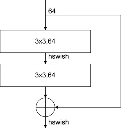
FIGURE 9. Residual block with the H-swish function.

FIGURE 10

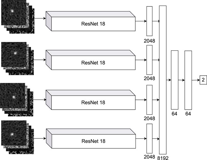
FIGURE 10. Rotational-invariant residual neural network.

We built the three-dimensional array by combining each candidate’s difference, template, science, and SNR stamps to feed the CNN models. For candidates from DIP, the array size is 91 × 91 × 4. For the candidates from QIP, the array size is 31 × 31 × 4 due to its 3 × 3 binned image properties. Before the CNN calculation, the pipeline rotates the stamp arrays 90, 180, and 270° to feed the four branches of our modified Deep-HiTS network. The main structure of our rotational invariant neural network is given in Figure 10.

Our convolutional parts used the modified ResNet-18 for feature extraction as the structure Table 1. The input channel is 4 to match the stamp arrays, and the output channel is 64 to feed the residual blocks. For the stamps with the 31 × 31 × 4 structure, the kernel size of the input layer is 3 × 3, and the stride step is 1 in the QIP. For the stamps with 91 × 91 × 4 from the DIP, the first layer used a 4 × 4 kernel size and stride steps of 3 to match the residual block inputs.

For each rotation of the stamp array, the modified ResNet-18 could create a vector of 2048 values as the feature extractions. We concatenated the output vectors of all rotations to a vector of 4 × 2048. The fully connected layers are constructed by three linear layers and two H-Swish activation functions. These feature values were classified into two fully-connected layers.

Due to the limitations of single-band observations, we only classified the candidates into positive and negative categories rather than performing a multicategory analysis. The classification of the results could be a binary problem that could use the simple cross-entropy loss function. The p(x) in the function represents the true value q(x) and represents the neural network classification value. The whole training problem of the neural network is, thus, to find the minimum cross-entropy under the training samples:

$H\left(p,q\right)=-\sum _{x}p\left(x\right)\log q\left(x\right).(6)$

4.2 Training and Accuracy

The CNN training requires an extensive data set to avoid overfitting. The training data set should preferably be a balanced sample for CNN models. However, it is impossible to construct a balanced sample from the observational data. The negative candidates generated by transient detection are enormous, while the positive candidates are very rare in comparison. Thus, we used the simulated positive candidates to address this imbalance problem.

To create the simulated positive candidates, we selected hundreds of science images with the best magnitude limits, lower airmass of observation, and an excellent full-width half maximum of detected stars. For each image, the space-variation PSF is generated by PSFEx from the aperture catalog with the same method described in PSF photometry. The PSF model is constructed with a stamp (VIGNET) size of 31 × 31 and a space-variation polynomial order of 3. We added the artificial stars to the selected images with magnitudes from 17.0 to 19.5 magnitudes at random positions. All positive candidates are selected with the human check and rejected for the wrong results.

The negative candidates are bogus stamps caused by the residuals of alignments, isolated random hot pixels after resampling, cosmic rays, saturation stars, and some failed fitting sources. The negative candidates are produced from the image subtraction pipeline with real images and also selected by humans. We cut the stamps for positive and negative candidates with the image subtraction pipeline. We constructed data sets with 10⁴ positive and 10⁴ negative candidates. Examples of the train set are shown in Figure 11.

FIGURE 11

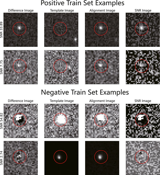
FIGURE 11. Examples of source samples for the positive and negative candidates used for training the neural networks.

Before the CNN training, we split 20% of candidates into the test group for training and validation groups. The rotational-invariant residual neural network trains with the optimizer AdamW, batches of 256 stamp arrays, and a dropout rate of 0.5 in the fully connected layer. The learning rate is set to a relatively low value of 0.01 at the beginning, and it steps down by multiplying by 0.9 after each epoch. We built the neural network with PyTorch (Paszke et al., 2019) and trained it on the NVIDIA A100 graphic processor unit. The training of our model requires a huge GPU memory, especially for the stamp size of 91 × 91 for the stamps from the DIP pipeline. The accuracies and precisions of the CNN models for QIP and DIP programs are shown in Table 3.

TABLE 3

TABLE 3. Precision of the CNN model for stamps from QIP and DIP.

4.3 Rotational-Invariant Residual Neural Network Performance

We calculated the false-negative rate (FNR) and the false-positive rate (FPR) with scikit-learn to analyze the neural network’s performance. The detection error trade-off (DET) curve demonstrates how FNR is correlated with FPR. The DET curves could show the performance of the CNN models used for candidate classification and provide direct feedback on the detection error trade-offs to help analyze the neural network. In Figure 12, we presented the DET curve for candidates in different signal-to-noise (SNR) groups. The higher SNR curve shows a quicker move to the bottom left, better fitting the plot.

FIGURE 12

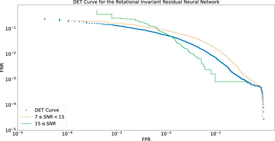
FIGURE 12. Blue dots show the detection error trade-off curve for the stamps from 3 × 3 binned images. The green and orange curves show the DET curve for different signal-to-noise ratio groups. The x-axis is the false negative rate, and the y-axis is the false positive rate.

Figure 12 shows that the rotational-invariant model is well-operated for the higher signal-to-noise ratio sources, which is in line with our expectations. The curve for higher SNR shows a vertical line, which may be caused by having only 10⁴ sources as positive stamps.

5 Conclusion

This article described the science data reduction pipeline and transient detection pipeline for the AST3-3 telescope at the Yaoan Observation Station. The science image pipeline uses the statistical method to estimate the quality of the observed image, taking into account the effects of poor weather, such as clouds passing through in the FoV.

The transient detection pipeline uses multiple binned and unbinned science images to extract the candidates faster and deeper. In terms of transient source detection, the robustness and flexibility of the program are improved through a combination of multiple detection methods and the CNN method. We introduced a rotation-invariant residual neural network to classify the candidate stamps from the transient detection pipeline. The CNN trained on the negative and simulated positive stamps cut. The CNN accuracy achieved 99.87% for the QIP and 99.20% for the DIP. AST3-3 has been designed for robotic observation and has a complete pipeline system with specific software, a well-trained CNN model, and management for the observation at the Yaoan Observation Station. This work allowed us to effectively participate in the LIGO-Virgo O4 ground optical follow-up observing campaign.

Data Availability Statement

The original contributions presented in the study are included in the article/supplementary material; further inquiries can be directed to the corresponding author.

Author Contributions

TS contributed to the design and whole system of the study. TS and LH organized the database of transient detection and classification. XL and KM worked on the hardware supplement. All authors contributed to manuscript revision and read and approved the submitted version.

Funding

This work is partially supported by the National Natural Science Foundation of China (Grant Nos. 11725314 and 12041306), the Major Science and Technology Project of Qinghai Province (2019-ZJ-A10), the ACAMAR Postdoctoral Fellow, the China Postdoctoral Science Foundation (Grant No. 2020M681758) and the Natural Science Foundation of Jiangsu Province (grant No. BK20210998). TS and AC also acknowledge financial support from the State Agency for Research of the Spanish MCIU through the “ Center of Excellence Severo Ochoa” award to the Instituto de Astrofísica de Andalucía (SEV-2017-0709). TS acknowledges the China Scholarship Council (CSC) for funding his PhD scholarship (202006340174).

Conflict of Interest

The authors declare that the research was conducted in the absence of any commercial or financial relationships that could be construed as a potential conflict of interest.

Publisher’s Note

All claims expressed in this article are solely those of the authors and do not necessarily represent those of their affiliated organizations, or those of the publisher, the editors, and the reviewers. Any product that may be evaluated in this article, or claim that may be made by its manufacturer, is not guaranteed or endorsed by the publisher.

Acknowledgments

The AST3-3 team would like to express their sincere thanks to the staff of the Yaoan Observation Station. The authors are also grateful to anonymous referees whose opinion has significantly improved this manuscript. This research has made use of data and services provided by the International Astronomical Union’s Minor Planet Center. This work has made use of data from the European Space Agency (ESA) mission Gaia (https://www.cosmos.esa.int/gaia), processed by the Gaia Data Processing and Analysis Consortium (DPAC, https://www.cosmos.esa.int/web/gaia/dpac/consortium). Funding for the DPAC has been provided by national institutions, in particular the institutions participating in the Gaia Multilateral Agreement. Software packages: this research made use of Astropy,¹ a community-developed core Python package for Astronomy (Astropy Collaboration et al., 2013, 2018). The python packages: L.A. Cosmic (van Dokkum et al., 2012), PyEphem (Rhodes, 2011), Skyfield (Rhodes, 2019), PyTorch (Paszke et al., 2019), scikit-image (Van der Walt et al., 2014), scikit-learn (scikit-learn developers, 2020), Matplotlib (Hunter, 2007), SciPy(Jones et al., 2001), statsmodels (Seabold and Perktold, 2010), sep (Barbary, 2016), and SFFT (Hu et al., 2021). Software programs: SExtractor (Bertin and Arnouts, 2010), SWarp (Bertin, 2010), Astrometry.net (Lang et al., 2012), FITSH (Pál, 2011), and fpack (Seaman et al., 2010).

Footnotes

¹http://www.astropy.org

References

Alard, C. (2000). Image Subtraction Using a Space-Varying Kernel. Astron. Astrophys. Suppl. Ser. 144, 363–370. doi:10.1051/aas:2000214

CrossRef Full Text | Google Scholar

Alard, C., and Lupton, R. H. (1998). A Method for Optimal Image Subtraction. ApJ 503, 325–331. doi:10.1086/305984

CrossRef Full Text | Google Scholar

Andreoni, I., Jacobs, C., Hegarty, S., Pritchard, T., Cooke, J., and Ryder, S. (2017). Mary, a Pipeline to Aid Discovery of Optical Transients, 34. New York: Publications of the Astron. Soc. of Australia, e037. doi:10.1017/pasa.2017.33

CrossRef Full Text | Google Scholar

Astropy Collaboration Price-Whelan, A. M., Price-Whelan, A. M., Sipőcz, B. M., Günther, H. M., Lim, P. L., Crawford, S. M., et al. (2018). The Astropy Project: Building an Open-Science Project and Status of the v2.0 Core Package. Aj 156, 123. doi:10.3847/1538-3881/aabc4f

CrossRef Full Text | Google Scholar

Astropy Collaboration Robitaille, T. P., Robitaille, T. P., Tollerud, E. J., Greenfield, P., Droettboom, M., Bray, E., et al. (2013). Astropy: A Community Python Package for Astronomy. A&A 558, A33. doi:10.1051/0004-6361/201322068

CrossRef Full Text | Google Scholar

Barbary, K. (2016). SEP: Source Extractor as a Library. Joss 1, 58. doi:10.21105/joss.00058

CrossRef Full Text | Google Scholar

Barthelmy, S. (2008). GCN and VOEvent: A Status Report. Astron. Nachr. 329, 340–342. doi:10.1002/asna.200710954

CrossRef Full Text | Google Scholar

Becker, A. C., Homrighausen, D., Connolly, A. J., Genovese, C. R., Owen, R., Bickerton, S. J., et al. (2012). Regularization Techniques for PSF-Matching Kernels - I. Choice of Kernel Basis. Mon. Notices R. Astronomical Soc. 425, 1341–1349. doi:10.1111/j.1365-2966.2012.21542.x

CrossRef Full Text | Google Scholar

Bertin, E., and Arnouts, S. (1996). SExtractor: Software for Source Extraction. Astron. Astrophys. Suppl. Ser. 117, 393–404. doi:10.1051/aas:1996164

CrossRef Full Text | Google Scholar

Bertin, E., and Arnouts, S. (2010). SExtractor: Source Extractor. Houghton, Michigan: Astrophysics Source Code Library. record ascl:1010.064.

Google Scholar

Bertin, E. (2013). PSFEx: Point Spread Function Extractor.

Google Scholar

Bertin, E. (2010). SWarp: Resampling and Co-adding FITS Images Together.

Google Scholar

Bramich, D. M. (2008). A New Algorithm for Difference Image Analysis. Mon. Not. Ras. Lett. 386, L77–L81. doi:10.1111/j.1745-3933.2008.00464.x

CrossRef Full Text | Google Scholar

Bramich, D. M., Horne, K., Albrow, M. D., Tsapras, Y., Snodgrass, C., Street, R. A., et al. (2013). Difference Image Analysis: Extension to a Spatially Varying Photometric Scale Factor and Other Considerations. Mon. Notices R. Astronomical Soc. 428, 2275–2289. doi:10.1093/mnras/sts184

CrossRef Full Text | Google Scholar

Brennan, S. J., and Fraser, M. (2022). The AUTOmated Photometry of Transients (AutoPhOT) Pipeline. arXiv e-prints, arXiv:2201.02635.

Google Scholar

Cabrera-Vives, G., Reyes, I., Förster, F., Estévez, P. A., and Maureira, J.-C. (2017). Deep-HiTS: Rotation Invariant Convolutional Neural Network for Transient Detection. ApJ 836, 97. doi:10.3847/1538-4357/836/1/97

CrossRef Full Text | Google Scholar

Calabretta, M., and Greisen, E. W. (2000). “Representations of World Coordinates in FITS,” Astronomical Society of the Pacific Conference Series. Editors N. Manset, C. Veillet, and D. Crabtree (San Francisco: Astronomical Data Analysis Softw. Syst. IX), 216, 571.

Google Scholar

Cao, Y., Nugent, P. E., and Kasliwal, M. M. (2016). Intermediate Palomar Transient Factory: Realtime Image Subtraction Pipeline, 128. Bristol: Publications of the ASP, 114502. doi:10.1088/1538-3873/128/969/114502

CrossRef Full Text | Google Scholar

Carrasco-Davis, R., Reyes, E., Valenzuela, C., Förster, F., Estévez, P. A., Pignata, G., et al. (2021). Alert Classification for the ALeRCE Broker System: The Real-Time Stamp Classifier. Aj 162, 231. doi:10.3847/1538-3881/ac0ef1

CrossRef Full Text | Google Scholar

Chambers, K. C.Pan-STARRS Team (2017). “The Pan-STARRS1 Survey Data Release,” in American Astronomical Society Meeting Abstracts #229 (American Astronomical Society Meeting Abstracts), 223–03.

Google Scholar

Craig, M. W., Crawford, S. M., Deil, C., Gomez, C., Günther, H. M., Heidt, N., et al. (2015). Ccdproc: CCD Data Reduction Software.

Google Scholar

Dálya, G., Díaz, R., Bouchet, F. R., Frei, Z., Jasche, J., Lavaux, G., et al. (2021). GLADE+: An Extended Galaxy Catalogue for Multimessenger Searches with Advanced Gravitational-Wave Detectors. arXiv e-prints, arXiv:2110.06184.

Google Scholar

Dieleman, S., Willett, K. W., and Dambre, J. (2015). Rotation-invariant Convolutional Neural Networks for Galaxy Morphology Prediction. Mon. Notices RAS 450, 1441–1459. doi:10.1093/mnras/stv632

CrossRef Full Text | Google Scholar

Förster, F., Maureira, J. C., San Martín, J., Hamuy, M., Martínez, J., Huijse, P., et al. (2016). The High Cadence Transient Survey (HITS). I. Survey Design and Supernova Shock Breakout Constraints. AstronoAstrophysical J. 832, 155. doi:10.3847/0004-637X/832/2/155

CrossRef Full Text | Google Scholar

Gaia Collaboration Brown, A. G. A., Vallenari, A., Prusti, T., de Bruijne, J. H. J., Babusiaux, C., Bailer-Jones, C. A. L., et al. (2018). Gaia Data Release 2. Summary of the Contents and Survey Properties. Astronomy Astrophysics 616, A1. doi:10.1051/0004-6361/201833051

CrossRef Full Text | Google Scholar

Goldstein, D. A., D’Andrea, C. B., Fischer, J. A., Foley, R. J., Gupta, R. R., Kessler, R., et al. (2015). Automated Transient Identification in the Dark Energy Survey. Astronomical J. 150, 82. doi:10.1088/0004-6256/150/3/8210.1088/0004-6256/150/5/165

CrossRef Full Text | Google Scholar

Gómez, C., Neira, M., Hernández Hoyos, M., Arbeláez, P., and Forero-Romero, J. E. (2020). Classifying Image Sequences of Astronomical Transients with Deep Neural Networks. Mon. Notices RAS 499, 3130–3138. doi:10.1093/mnras/staa2973

CrossRef Full Text | Google Scholar

Greenfield, P., Robitaille, T., Tollerud, E., Aldcroft, T., Barbary, K., Barrett, P., et al. (2013). Astropy. Houghton, Michigan: Community Python library for astronomy.

Google Scholar

He, K., Zhang, X., Ren, S., and Sun, J. (2015). Deep Residual Learning for Image Recognition. arXiv e-prints, arXiv:1512.03385.

Google Scholar

Hochreiter, S., and Schmidhuber, J. (1997). Long Short-Term Memory. Neural Comput. 9, 1735–1780. doi:10.1162/neco.1997.9.8.1735

PubMed Abstract | CrossRef Full Text | Google Scholar

Howard, A., Sandler, M., Chu, G., Chen, L.-C., Chen, B., Tan, M., et al. (2019). Searching for MobileNetV3. arXiv e-prints, arXiv:1905.02244.

Google Scholar

Hu, L., Wang, L., and Chen, X. (2021). Image Subtraction in Fourier Space. arXiv e-prints, arXiv:2109.09334.

Google Scholar

Hu, L., Wang, L., and Chen, X. (2021). Sfft. doi:10.5281/zenodo.5521634

CrossRef Full Text | Google Scholar

Hunter, J. D. (2007). Matplotlib: A 2D Graphics Environment. Comput. Sci. Eng. 9, 90–95. doi:10.1109/mcse.2007.55

CrossRef Full Text | Google Scholar

Irwin, J., Irwin, M., Aigrain, S., Hodgkin, S., Hebb, L., and Moraux, E. (2007). The Monitor Project: Data Processing and Light Curve Production. Mon. Notices RAS 375, 1449–1462. doi:10.1111/j.1365-2966.2006.11408.x

CrossRef Full Text | Google Scholar

Jia, P., Zhao, Y., Xue, G., and Cai, D. (2019). Optical Transient Object Classification in Wide-Field Small Aperture Telescopes with a Neural Network. Aj 157, 250. doi:10.3847/1538-3881/ab1e52

CrossRef Full Text | Google Scholar

Jones, E., Oliphant, T., and Peterson, P. (2001). SciPy: Open Source Scientific Tools for Python.

Google Scholar

Kashyap, V. L., van Dyk, D. A., Connors, A., Freeman, P. E., Siemiginowska, A., Xu, J., et al. (2010). On Computing Upper Limits to Source Intensities. ApJ 719, 900–914. doi:10.1088/0004-637X/719/1/900

CrossRef Full Text | Google Scholar

Lang, D., Hogg, D. W., Mierle, K., Blanton, M., and Roweis, S. (2012). Astrometry.net: Astrometric Calibration of Images. Houghton, Michigan: Astrophysics Source Code Library. record ascl:1208.001.

Google Scholar

Lang, D., Hogg, D. W., Mierle, K., Blanton, M., and Roweis, S. (2010). Astrometry.net: Blind Astrometric Calibration of Arbitrary Astronomical Images. Astronomical J. 139, 1782–1800. doi:10.1088/0004-6256/139/5/1782

CrossRef Full Text | Google Scholar

Lecun, Y., Bengio, Y., and Hinton, G. (2015). Deep Learning. Nature 521, 436–444. doi:10.1038/nature14539

PubMed Abstract | CrossRef Full Text | Google Scholar

Li, X., Yuan, X., Gu, B., Yang, S., Li, Z., and Du, F. (2019). “Chinese Antarctic Astronomical Optical Telescopes,” in Revista Mexicana de Astronomia y Astrofisica Conference Series (Mexico: Revista Mexicana de Astronomia y Astrofisica Conference Series), 51, 135–138. doi:10.22201/ia.14052059p.2019.51.23

CrossRef Full Text | Google Scholar

Loshchilov, I., and Hutter, F. (2017). Decoupled Weight Decay Regularization. arXiv e-prints arXiv:1711.05101.

Google Scholar

Masci, F. J., Laher, R. R., Rusholme, B., Shupe, D. L., Groom, S., Surace, J., et al. (2019). The Zwicky Transient Facility: Data Processing, Products, and Archive, 131. Bristol: Publications of the ASP, 018003. doi:10.1088/1538-3873/aae8ac

CrossRef Full Text | Google Scholar

Mommert, M. (2017). PHOTOMETRYPIPELINE: An Automated Pipeline for Calibrated Photometry. Astronomy Comput. 18, 47–53. doi:10.1016/j.ascom.2016.11.002

CrossRef Full Text | Google Scholar

Morganson, E., Gruendl, R. A., Menanteau, F., Kind, M. C., Chen, Y.-C., Daues, G., et al. (2018). The Dark Energy Survey Image Processing Pipeline, 130. Bristol: Publications of the ASP, 074501. doi:10.1088/1538-3873/aab4ef

CrossRef Full Text | Google Scholar

Nair, V., and Hinton, G. E. (2010). Rectified Linear Units Improve Restricted Boltzmann Machines. ICML, 807–814.

Google Scholar

National Optical Astronomy Observatories (1999). IRAF: Image Reduction and Analysis Facility.

Google Scholar

Paillassa, M., Bertin, E., and Bouy, H. (2020). MAXIMASK and MAXITRACK: Two New Tools for Identifying Contaminants in Astronomical Images Using Convolutional Neural Networks. A&A 634, A48. doi:10.1051/0004-6361/201936345

CrossRef Full Text | Google Scholar

Pál, A. (2012). FITSH- a Software Package for Image Processing. Mon. Notices RAS 421, 1825–1837. doi:10.1111/j.1365-2966.2011.19813.x

CrossRef Full Text | Google Scholar

Pál, A. (2011). FITSH: Software Package for Image Processing. Houghton, Michigan: Astrophysics Source Code Library. record ascl:1111.014.

Google Scholar

Paszke, A., Gross, S., Massa, F., Lerer, A., Bradbury, J., Chanan, G., et al. (2019). “Pytorch: An Imperative Style, High-Performance Deep Learning Library,” in Advances in Neural Information Processing Systems 32. Editors H. Wallach, H. Larochelle, A. Beygelzimer, F. d’ Alché-Buc, E. Fox, and R. Garnett (Cambridge, MA: Curran Associates, Inc.), 8024–8035.

Google Scholar

Pearson, K., and Galton, F. (1895). Vii. Note on Regression and Inheritance in the Case of Two Parents. Proc. R. Soc. Lond. 58, 240–242. doi:10.1098/rspl.1895.0041

CrossRef Full Text | Google Scholar

Pence, W. D., Seaman, R., and White, R. L. (2009). Lossless Astronomical Image Compression and the Effects of Noise, 121. Bristol: Publications of the ASP, 414–427. doi:10.1086/599023

CrossRef Full Text | Google Scholar

Price, P. A., and Magnier, E. A. (2019). Pan-STARRS PSF-Matching for Subtraction and Stacking. arXiv e-prints.

Google Scholar

Rhodes, B. C. (2011). PyEphem: Astronomical Ephemeris for Python.

Google Scholar

Rhodes, B. (2019). Skyfield: High Precision Research-Grade Positions for Planets and Earth Satellites Generator. Houghton, Michigan: Astrophysics Source Code Library. record ascl:1907.024.

Google Scholar

Rumelhart, D. E., Hinton, G. E., and Williams, R. J. (1986). Learning Representations by Back-Propagating Errors. Nature 323, 533–536. doi:10.1038/323533a0

CrossRef Full Text | Google Scholar

scikit-learn developers (2020). Scikit-learn : Machine Learning in Python.

Google Scholar

Seabold, S., and Perktold, J. (2010). “Statsmodels: Econometric and Statistical Modeling with python,” in 9th Python in Science Conference. doi:10.25080/majora-92bf1922-011

CrossRef Full Text | Google Scholar

Seaman, R., Pence, W., and White, R. (2010). Fpack: FITS Image Compression Program.

Google Scholar

Shupe, D. L., Moshir, M., Li, J., Makovoz, D., Narron, R., and Hook, R. N. (2005). “The SIP Convention for Representing Distortion in FITS Image Headers,”In Astronomical Data Analysis Software and Systems XIV. Editors P. Shopbell, M. Britton, and R. Ebert (San Francisco: Astronomical Society of the Pacific Conference Series), 347, 491.

Google Scholar

Sokolovsky, K. V., and Lebedev, A. A. (2018). VaST: A Variability Search Toolkit. Astronomy Comput. 22, 28–47. doi:10.1016/j.ascom.2017.12.001

CrossRef Full Text | Google Scholar

Van der Walt, S., Schönberger, J. L., Nunez-Iglesias, J., Boulogne, F., Warner, J. D., Yager, N., et al. (2014). Scikit-Image: Image Processing in python. PeerJ 2, e453. doi:10.7717/peerj.453

PubMed Abstract | CrossRef Full Text | Google Scholar

van Dokkum, P. G., Bloom, J., and Tewes, M. (2012). L.A.Cosmic: Laplacian Cosmic Ray Identification. Houghton, Michigan: Astrophysics Source Code Library. record ascl:1207.005.

Google Scholar

van Dokkum, P. G. (2001). Cosmic-Ray Rejection by Laplacian Edge Detection, 113. Bristol: Publications of the ASP, 1420–1427. doi:10.1086/323894

CrossRef Full Text | Google Scholar

Yin, K., Jia, J., Gao, X., Sun, T., and Zhou, Z. (2021). Supernovae Detection with Fully Convolutional One-Stage Framework. Sensors 21, 1926. doi:10.3390/s21051926

PubMed Abstract | CrossRef Full Text | Google Scholar

Yuan, X., Cui, X., Wang, L., Gu, B., Du, F., Li, Z., et al. (2015). The Antarctic Survey Telescopes AST3 and the AST3-NIR. IAU General Assem. 29, 2256923.

Google Scholar

Zhang, J.-C., Wang, X.-F., Mo, J., Xi, G.-B., Lin, J., Jiang, X.-J., et al. (2020). The Tsinghua University-Ma Huateng Telescopes for Survey: Overview and Performance of the System, 132. Bristol: Publications of the ASP, 125001. doi:10.1088/1538-3873/abbea2

CrossRef Full Text | Google Scholar

Zhang, T.-M., Wang, X.-F., Chen, J.-C., Zhang, J.-J., Zhou, L., Li, W.-X., et al. (2015). The THU-NAOC Transient Survey: the Performance and Results from the First Year. Res. Astron. Astrophys. 15, 215–224. doi:10.1088/1674-4527/15/2/006

CrossRef Full Text | Google Scholar